A Deep Reinforcement Learning-Based Partitioning Method for Power System Parallel Restoration

1  Introduction

Power systems are vulnerable to outages caused by natural disasters, equipment failures, and other factors. Notable examples include the widespread blackout in Spain and Portugal on 28 April 2025, the power outage in the UK in 2019 [1], several major power outages in Europe in 2021 [2], and the power outage in Texas, America, in 2021 [3]. Consequently, it is crucial to develop and implement rapid restoration techniques to reduce outage duration and reduce outage losses. Restoration modes generally include sequential restoration and parallel restoration. Since sequential restoration follows a single restoration path and often entails prolonged restoration times, it is unsuitable for large-scale outages. In contrast, parallel restoration accelerates the restoration process by simultaneously restoring multiple subsystems [4].

In recent years, research on parallel restoration strategies has garnered increasing attention. By dividing a power system outage into multiple independent subsystems, restoration efforts can be initiated simultaneously among these subsystems, thereby reducing the overall outage duration. Developing efficient partitioning schemes is central to parallel restoration in power systems and warrants further study. Various methods have been proposed to address this partitioning problem, including complex network theory, graph theory, mathematical programming, and intelligent methods.

Based on the complex network theory, Zou and Li [5] used an improved Fast–Newman algorithm and a weighted modular Q function to optimize the system partitioning. However, the method failed to consider the power balance within the subsystem. The virus propagation model is categorized as a propagation-dynamics algorithm within the framework of complex network theory. Since Huang et al. [6] proposed a partitioning method based on the susceptible–infected–recovered model, where different blackstart resource was regarded as “virus sources,” their propagation paths determined the formation of subsystems. However, the infection rates in the method are challenging to set accurately, which may lead to deviations in the partitioning result. Yang et al. [7] proposed an improved GN-based partitioning method for community detection methods. However, the improved GN algorithm relied on edge betweenness and system strength weights, which resulted in relatively high computational complexity. Yang et al. [8] proposed a balanced-depth algorithm to accelerate partitioning for a power system. Case study results showed that, compared with other partitioning methods, this algorithm achieved higher efficiency and generated higher-quality partitioning results. And by introducing the electrical coupling strength (ECS) and an improved Fast–Neumann algorithm, Zhao et al. [9] optimized the partitioning quality. However, the impact of variations in the ECS parameter on the partitioning result was not discussed. Moreover, constraints such as the balance of subsystem sizes were not considered. As a simple and efficient community detection algorithm, the Label Propagation Algorithm (LPA) was also applied to partition a power system [10,11]. Wei et al. [10] proposed a method based on the LPA combined with cooperative game theory. By introducing the Shapley value of buses, reference [10] realized a cooperative game strategy process between buses and subsystems to prevent label oscillations. However, cooperative game theory requires enumerating all possible combinations of nodes and subsystems, resulting in a computational burden for large systems. To address the oscillation problem commonly encountered in the LPA, Huang et al. [11] proposed an efficient method that introduced a strategy where labels influenced their buses to avoid oscillations. However, reference [11] used an exhaustive search method to refine the partitioning strategy, which could lead to low computational efficiency. Sun et al. [12] proposed a two-stage power grid partitioning strategy that integrates grid structural features and node voltage characteristics. Yet, the optimization adjustments during the partitioning process significantly increase computational complexity.

Based on the graph theory, Li et al. [13] used the minimum spanning tree algorithm to construct the power system network backbone with the shortest restoration time. At the same time, schedulable loads were considered to address the minimum power output constraints of generators. However, generating candidate partitioning schemes through exhaustive enumeration and evaluating them individually could increase computational complexity and affect scalability. Ganganath et al. [14] proposed a partitioning method for the power system using a three-step strategy, including initialization modeling, constraint satisfaction, and greedy clustering. However, this partitioning model did not consider the size balance constraint among subsystems, which may result in a certain subsystem becoming excessively large. Spectral clustering algorithms in graph theory have been applied to power system partitioning. For instance, Sarmadi and Dobakhshari [15] proposed the partitioning method based on spectral clustering; Hu et al. [16] proposed an improved spectral clustering-based partitioning method that addresses the sensitivity to initial values; Feng et al. [17] proposed a spectral clustering-based partitioning method that accounts for wind power integration. Chakrabarty et al. [18] proposed a partitioning based on K-means clustering. Yet this method depends on pre-outage system topology and heuristic rules. However, the spectral clustering algorithms involve significant eigenvalue decomposition, which increases computational complexity. Kyesswa et al. [19] investigated the performance differences of several partitioning methods (KaFFPa, spectral clustering, and METIS) in AC optimal power flow and dynamic power system simulation. The study showed that the KaFFPa partitioning algorithm outperformed other methods regarding computational speed and scalability.

The partitioning problem is usually treated as an optimization problem. Jiang and Ortmeyer [20] used a propagation-based mixed-integer linear programming method, considering power balance constraints between various types of generators and loads. However, this method is complex and relies on detailed mathematical modeling. Wu et al. [21] proposed a partitioning method based on mixed-integer nonlinear programming, which assigned blackstart resources and load buses to each subsystem according to electrical distance and power flow tracing results, while progressively satisfying the power balance within each subsystem. Wang et al. [22] proposed a partitioning method for a power system based on the location of blackstart resources, while employing the ADMN algorithm to coordinate power exchange among subsystems. Hartmann et al. [23] proposed a quantum optimization-based power grid partitioning method. However, hardware constraints and high sensitivity to parameters limit its applicability. Li et al. [24] developed a partitioning model based on mixed-integer linear programming, solving it using the Normalized Normal Constraint and the Variation Coefficient method. However, this study did not sufficiently discuss the impact of parameter variations on the partitioning result. Hartmann et al.

Based on the intelligent algorithms, Talib et al. [25] proposed a partitioning method based on the heuristic search for lower total restoration time. The method searched for suitable cut sets to balance the restoration time of each subsystem as much as possible. Thereby, the overall restoration speed was improved. However, the method relied on preset heuristic rules, making it less adaptable to power systems with different structures. Sun et al. [26] proposed a two-step grid-connected restoration partitioning strategy. First, a grouping model for the resource is established. Then, based on graph theory, the power system is partitioned to minimize interconnections between subsystems. However, the model has a relatively high computational complexity. Huo et al. [27] proposed a load restoration optimization strategy based on power system partitioning. The partitioning problem was solved by using an improved genetic algorithm. However, the limitations of the genetic algorithm may lead to local optima in some cases. Pan and Zhang [28] proposed a flexible blackstart partitioning method for a power system, introducing a subsystem restoration time balance index. However, the method is relatively sensitive to initial data and heuristic rules.

With the rapid development of artificial intelligence technologies in recent years, several researchers have applied DRL algorithms to solve power system problems. DRL performs well in solving complex decision-making tasks as an adaptive optimization algorithm. Thus, DRL has gradually been applied in making decisions for power system restoration [29–31]. Du and Wu [29] used expert demonstration data to improve the agent’s learning efficiency, avoid random exploration risks, and optimize microgrid restoration decisions. Hosseini et al. [30] used the Soft Actor-Critic algorithm to train local controllers for distributed resources, enabling swift and accurate power restoration operations facing uncertainties. Igder and Liang [31] used the Deep Q-Network (DQN) method for microgrid service restoration, allowing the agent to select the optimal restoration path and achieve efficient power restoration. In summary, DRL has performed excellently in solving power system problems. The existing methods for partitioning have relatively high computational complexity, or the algorithms easily fall into local optimal solutions.

This paper proposes a novel partitioning method for power system restoration based on DRL. The agent’s partitioning decision process involves identifying subsystem boundaries and assigning nodes to different subsystems. By considering the distribution of blackstart resources, the balance of node number among subsystems, and the power balance of the subsystem, this method can generate a power system partitioning scheme for parallel restoration.

The main contributions are as follows:

•   The partitioning decision process for power system parallel restoration is first modeled as a Markov Decision Process (MDP). According to partitioning characteristics, the state and action spaces are constructed for reasonable partitioning schemes.

•   A novel partitioning method based on DRL is proposed. Through trial and error, the agent can find the optimal subsystem boundaries to partition the blackout system rapidly.

•   The sensitivity of DRL parameters to the partitioning decision process is evaluated. The significant influence of varying discount factors on the training process of the partitioning decision has been experimentally verified.

The rest of this paper is organized as follows. Section 2 introduces the partitioning model of power system parallel restoration. Section 3 formulates the partitioning decision process of power systems as an MDP model. Section 4 solves the partitioning model of power systems using the DRL algorithm. Section 5 uses the IEEE 39-bus test system for partitioning simulation to verify the effectiveness of the proposed method. Section 6 is a summary of this paper.

2  Partitioning Model for Power System Parallel Restoration

Based on graph theory, a power system can be abstracted as a graph composed of edges and nodes, where the edges represent transmission lines or transformers, and the nodes represent power plant-, substation-, or load-buses. Partitioning tasks are to find the boundary edges among subsystems or to divide nodes into different subsystems.

Reasonable partitioning for power systems following blackouts is helpful for effective parallel restoration of multiple subsystems. According to the partitioning strategy, each subsystem can restore itself independently and quickly. Thus, this section proposes the partitioning model for power system parallel restoration to maximize modularity, subject to constraints including balance of node number among subsystems, distribution of blackstart resources, and power balance within each subsystem. The derived subsystems are generated by solving the proposed model for parallel restoration.

It assumes that the power system topology remains unchanged after blackouts. Dual-circuit lines or multiple-circuit lines are treated as single-circuit lines. Since the restoration task is to restore the outage system to its state as much as possible before the outage, the loads do not consider the fluctuations throughout the day.

2.1 Objective

Modularity is an important metric used to measure network partitioning and evaluate the quality of node division within a network [32]. According to the community detection theory, modularity effectively captures the strength of connections among subsystems and nodes within each subsystem. This paper uses modularity as the partitioning objective for a power system to measure the partitioning quality. According to [33], modularity can be calculated as follows:

Q=12m∑i=1n∑j=1n(Aij−kikj2m)δ(ci,v1,cj,v2),(1)

where m is the total number of edges in the network, A is the adjacency matrix; ki represents the number of adjacent nodes connected to node i, ci,v1 indicates that node v1 is in subsystem Si. The function δ represents the partitioning relationship between nodes, and its formula is as follows:

δ(ci,v1,cj,v2)={1,v1 and v2are in the same subsystem0,v1 and v2are not in the same subsystem.(2)

Generally, higher modularity indicates a more reasonable partitioning, with stronger connections between nodes within the subsystem. For the actual network, Newman pointed out that good network partitioning typically has a modularity Q ranging from 0.3 to 0.7 [34].

2.2 Constraints

2.2.1 Balance Constraint on Node Number among Subsystems

For power system parallel restoration, if one subsystem contains too many nodes, restoring itself demands many operational steps, thereby extending restoration time and consuming more restoration resources. Conversely, a subsystem with too few nodes may finish too early and sit idle. Significant deviations can cause the overall restoration progress to be held back by the slowest subsystem. Balancing the node number among subsystems can ensure that each subsystem’s restoration workload is comparable. Load restoration in every subsystem completes roughly the same time, optimizing the deployment of resources and maximizing parallel restoration efficiency. The constraint for balanced node number is as follows:

Navg=⌈Vk⌉,(3)

|Si|=∑v∈Vzi,v,(4)

Navg−Δ≤∑v∈Vzi,v≤Navg+Δ,(5)

where Navg represents the average number of nodes each subsystem; V represents the number of nodes in the power system; ⌈•⌉ represents the ceiling of a value; |Si| represents the sum of nodes within subsystem Si; zi,v = 1 represents that node v belongs to subsystem Si; and Δ is an allowable deviation value. Eq. (5) represents the threshold for the number of nodes within each subsystem.

2.2.2 Distribution Constraint of Blackstart Resource

Each subsystem should have blackstart resources to restore itself. Thus, the number of subsystems is not larger than the number of blackstart resources. Moreover, every node should be connected to one subsystem to restore all nodes. This equation ensures that each node belongs to exactly one subsystem. And the number of subsystems does not exceed the number of blackstart resources. The distribution constraint of blackstart resources is as follows:

|S1|∪|S2|∪⋯∪|SK|=V,(6)

|Si|∩|Sj|=∅,∀i≠j,(7)

K≤NBS,(8)

where NBS represents the number of blackstart resources. ∪ represents the union operation; ∩ represents the intersection operation; ∀ represents the number of any given subsystem.

Each subsystem should include a blackstart resource to ensure that each subsystem can self-initiate and restore [35]. The formula for each subsystem with only one blackstart resource is as follows:

xv={1,while node v is ; blackstart resource node0, Otherwise,(9)

∑v∈Sixv=1,∀i∈{1,2,…,K},K≤NBS.(10)

2.2.3 Power Balance Constraint in the Subsystem

If the generator capacity is insufficient in each subsystem, it cannot provide adequate cranking power to restore all loads. Consequently, the maximum power of the generators within each subsystem must be larger than the demand of the loads. The power balance constraint is as follows:

PSigen≥PSiload,∀i∈{1,2,…,k},(11)

where PSigen represents the total output power of generators within subsystem Si, while PSiload represents the total load power within subsystem Si.

3  MDP Formulation of the Partitioning Decision Process

The decision process is modeled as an MDP based on the partitioning process’s characteristics. The assignment of nodes to subsystems is regarded as the MDP’s state space, while the set of edges is viewed as its action space. The MDP’s reward function is designed.

3.1 Fundamental Concepts of MDP

MDP is a process in which the agent continuously interacts with the environment, gradually optimizing its decision policy to achieve a specific goal. MDP can be represented as follows:

MDP={S,A,P,r,γ},(12)

where S represents the state space; A represents the action space; P represents the transition probability from current state s to next state s′ with performing action a; r represents the obtained reward from state s to state s′ with performing action a; and γ represents the discount factor.

MDP aims to find the optimal policy π that maximizes the cumulative reward. One characteristic of MDP is the Markov property, which means that the next state of the system depends only on the current state and the current action.

The partitioning scheme comprises a series of edge actions, which influence the assignment of nodes to subsystems. The affiliation state of nodes only depends on the node affiliation state and action at the previous moment, and is irrelevant to historical states. Therefore, the partitioning decision process for a power system conforms to the Markov property since the process can be modeled as an MDP.

3.2 Design of State Space

The partitioning decision process focuses on the problem of node assignment to subsystems and subsystem boundaries. Therefore, this paper defines the state of node assignments to subsystems and the state of edges serving as subsystem boundaries as the state space of the MDP. The state of a node is defined as follows:

f(v)∈{1,2,…,NBS},v∈V,(13)

where f(v) represents the subsystem index to which node v belongs. For instance, f(1) = 2 represents that node 1 belongs to subsystem 2. When a node has not been partitioned, the node’s state is defined as f(v) = −1.

The state of branches serving as subsystem boundaries is as follows:

N=(N0,N1,…,Nl−1),l≤L(14)

where Nl = 0 represents that branch l is not the subsystem boundary, Nl = 0 represents that branch l serves as the subsystem boundary; L represents the total number of edges for the power grid. N represents the branch state vector, a 1 × N vector.

According to Eqs. (13) and (14), the state space is defined as follows:

S=[f(1),f(2),…,f(v),N],(15)

where the position of f(v) in the state space is determined by node v. For a power system network with V nodes and L edges, the state space is represented as 1 row and (V + N) columns. The f(v) should be assigned to row 1, column v of the state space.

To better explain the state space, this paper uses a 7-bus topology as an example. The initial topology is shown in Fig. 1.

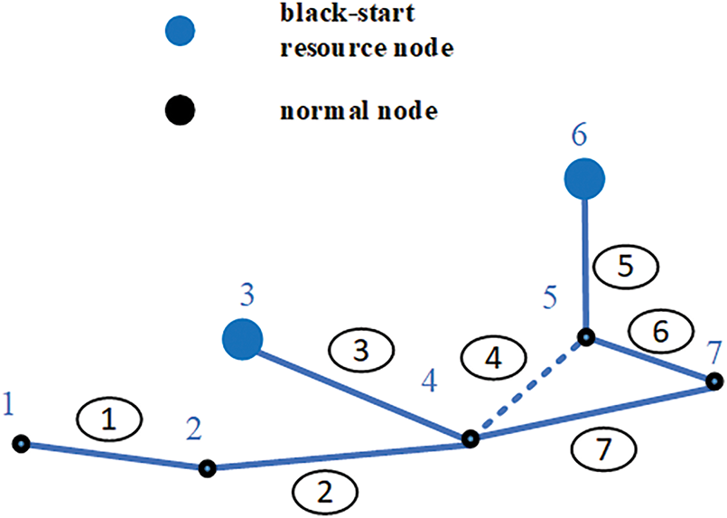
Figure 1: 7-bus topology

As shown in Fig. 1, the black nodes are normal nodes, and the blue nodes indicate the locations of blackstart resources. And the power grid has 7 nodes and 7 edges. Blackstart resources are located at node 3 and node 6. Nodes directly connected only to the blackstart resource at node 3 are assigned to Subsystem 1, while nodes connected only to the blackstart resource at node 6 are assigned to Subsystem 2. Fig. 2 shows three scenarios in the partitioning process.

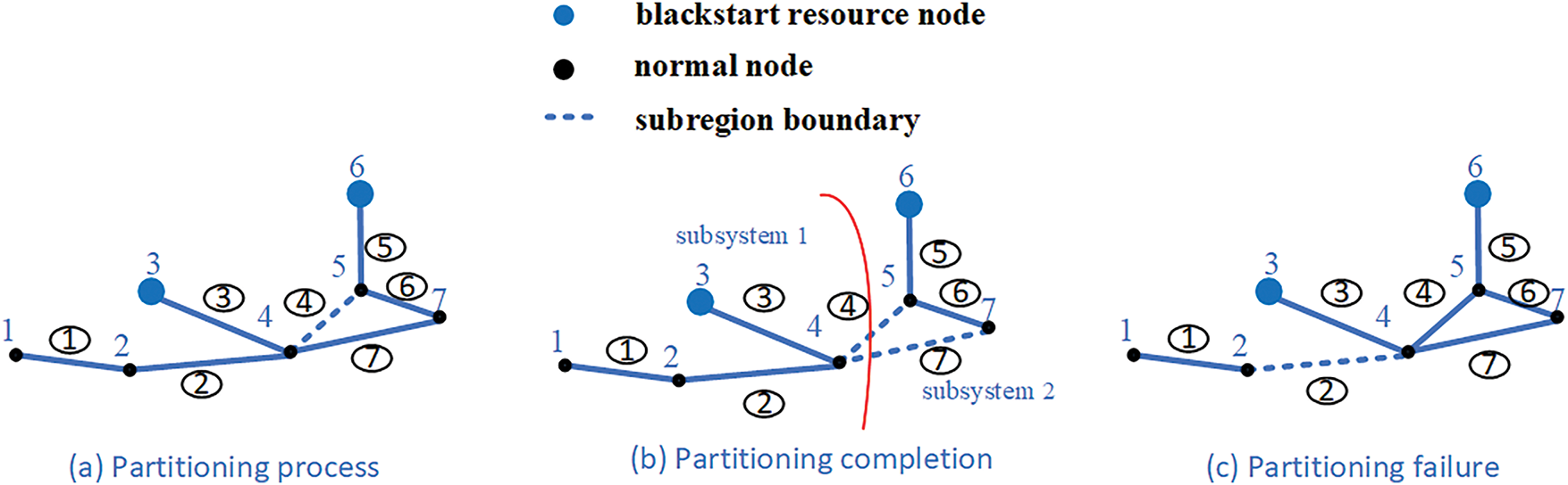
Figure 2: Three scenarios in the partitioning process

The evolution of the state space is as follows:

(1)   As shown in Fig. 1, all nodes are simultaneously connected to all blackstart resource nodes at this stage. Nodes belong to no subsystem yet; thus, f(1) and f(7) are all set to −1. No edges have been selected as subsystem boundaries, hence N = (0, 0, 0, 0, 0, 0, 0). The state vector is S = [−1, −1, −1, −1, −1, −1, −1, N].

(2)   As shown in scenario (a) of Fig. 2, all nodes remain connected to all blackstart sources, thus f(1) to f(7) remain the status of −1. The agent has selected edge 4 as a subsystem boundary, hence N = (0, 0, 0, 1, 0, 0, 0).

(3)   As shown in scenario (b) of Fig. 2, the agent has selected edges 4 and 7 as subsystem boundaries, thus N = (0, 0, 0, 1, 0, 0, 1). All nodes are connected exclusively to a blackstart resource, hence f(1) to f(4) = −1 and f(5) to f(7) = 2. The state vector is S = [1, 1, 1, 1, 2, 2, 2, N].

(4)   As shown in scenario (c) of Fig. 2, nodes 1 and 2 are disconnected from all blackstart resources, resulting in an “islanding” phenomenon of these nodes. Consequently, this state is regarded as a partitioning failure.

3.3 Design of Action Space

Action space represents the set of all possible actions the agent can take. Careful design of the action space is critical in DRL. A huge action space may significantly increase computational complexity, whereas an overly constrained one could hinder the agent’s ability to accomplish the designated task. A well-designed action space of appropriate size can facilitate more efficient exploration by the agent.

Thus, this paper defines the number of edges in the power system as the action space, each representing one action. In this way, the action that the agent selects serves as the subsystem’s boundary. The connectivity of the generated subsystems can be ensured by using edge actions to partition the power system. The method facilitates the agent in generating a reasonable partitioning scheme with fewer actions. The definition of action space is as follows:

A=E,(16)

where E represents the set of all edges in the network.

3.4 Design of Reward Function

The reward function evaluates the agent’s value from performing a specific action. This paper designs the reward function based on the objective and constraints of the partitioning model for power systems. Among them, the objective serves as the reward term of the reward function, and the constraints serve as the penalty terms.

Regarding the reward and penalty terms in the reward function, the manuscript adopts a relative deviation normalization scheme to compress the value of each term to the range [0, 1). Since the modularity Q value naturally falls within the range of 0 to 1, the reward term for modularity Q does not need to be normalized. To avoid the overestimation of Q-values, this paper adopts the soft bonus scaling mechanism to construct the reward function, as follows:

RQ={Q,Q<QmaxQ+αtanh⁡(Q−Qmaxφ),Q>=Qmax,(17)

where α is a constant and represents the reward component of the reward function for guiding the agent towards higher partition quality decisions. φ limits the magnitude of the additional reward. The tanh () is the hyperbolic tangent function, which ensures a continuous transition of the additional reward from 0 to 1 and prevents huge numerical jumps.

For the penalty term about node deviation among subsystems, the unnormalized node penalty term will play a dominant role if the node deviation is too large. In contrast, the other terms will be ignored. Therefore, the penalty term Rnode needs to be normalized, as follows:

Rnode={−|Si|−Navg|Si|,|Si|−Navg>Δ−Navg−|Si|Navg,Navg−|Si|>Δ0,||Si|−Navg|<Δ,(18)

where |Si| represents the node number of subsystem Si. ∆ represents the deviation threshold for the node number of subsystems. Eq. (18) ensures the penalty term Rnode is within [0, 1]. A corresponding penalty is applied based on the deviation of the node number. If the deviation between the subsystem node number and the average node number is exceptionally large, Rnode approximately equals to 1. Conversely, if the deviation nears the predefined threshold ∆, Rnode converges to 0.

For the penalty term about power balance within each subsystem, Rpower also needs to be normalized, as follows:

Rpower={0,PSigen≥PSiload−PSiload−PSigenPSiload,PSigen<PSiload.(19)

Eq. (19) ensures the penalty term Rpower within [0, 1). A corresponding penalty is applied based on the deviation of the power balance. If the deviation between the PSiload and PSigen within each subsystem is very large, Rpower approximately equals 1. Conversely, if the deviation approaches 0, Rpower converges to 0.

Based on Eqs. (17)–(19), the final reward function formula for the power system partition model is obtained as follows:

R(s,a)=RQ+Rnode+Rpower.(20)

According to Foraboschi [36], there are differences between the mathematical models in engineering and physical models. Therefore, mathematical models require built-in fault tolerance. Inspired by the paper, this MDP reward function incorporates tolerance considerations. For example, Eq. (17) achieves smooth transitions in modularity through the hyperbolic tangent function tanh (); Eq. (18) permits the agent to generate partitioning scheme within node-number deviation threshold Δ; Eq. (19) dynamically adjusts penalty severity through proportional deviations, guiding the agent to ensure that generated subsystems satisfy power balance constraints, thus guaranteeing engineering tolerance in the partitioning model.

4  Partitioning Method Based on Deep Reinforcement Learning

Reinforcement learning is a typical algorithm for solving MDP models. Therefore, the paper uses relevant DRL algorithms to solve the partitioning model for power system parallel restoration.

The model is solved using the DQN algorithm in deep reinforcement learning. First, reinforcement learning and the DQN algorithm are introduced. Then, the experience replay buffer of the DQN algorithm is designed. Finally, the interaction process between the DQN algorithm and the power system environment is explained.

4.1 DQN Algorithm

The interaction process between deep reinforcement learning and the environment is shown in Fig. 3.

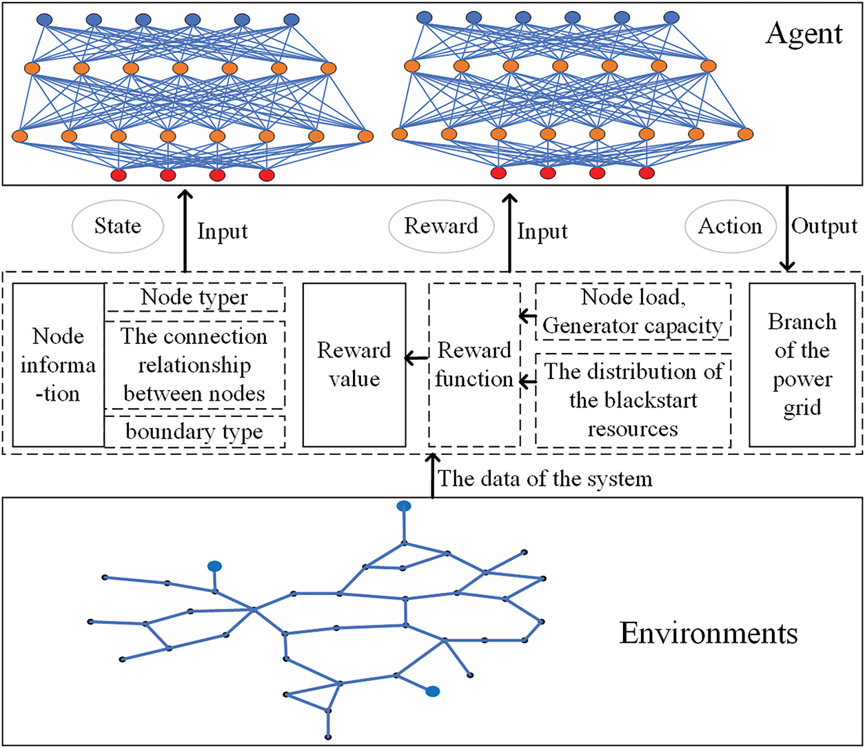
Figure 3: The process of deep reinforcement learning

As shown in Fig. 3, the agent interacts with the environment through states, actions, and rewards. The state space and reward function determine the input data for agent training or decision-making. The action space determines the output data for agent decision-making. Among them, the state space’s node information and boundary types are used as the agent’s input data; the reward value is obtained based on the node load, generator capacity, and the distribution of blackstart resources; the action is selected from the branch of the power grid. First, the power grid environment serves as data input. The data that the agent receives is used to make decisions. Subsequently, the agent outputs an action to act on the environment. Following this, the reward value is calculated according to Eqs. (17) to (20). The obtained reward value in each training episode serves as the agent’s input, guiding the agent to perform the next action. The updated grid environment and generated reward are then fed to the agent, initiating the next interaction cycle.

As an algorithm in deep reinforcement learning, DQN combines Q-learning with deep neural networks. In Q-learning, the value function Q(s, a) is used to evaluate the value of an action. Moreover, the function Q(s, a) serves as a bridge between states and actions. The formula for the value of Q is as follows:

Q(s,a)=r(s,a)+Eτ∼π[γmaxa′∈A⁡Q(s′,a′](21)

where γ is the discount factor; A is the action space; r(s, a) represents the immediate reward obtained when taking action a in state s, directly reflecting the interaction results between the agent and the environment. Eτ∼π[...] represents the average Q-value for all possible subsequent states under policy π. τ represents the subsequent state transitions under policy π; Q(s, a) represents the expected value obtained after transitioning to the next state by taking action a in state s.

The deep neural network can effectively process data, and its ability to update parameters allows it to better adapt to changes in the environment, thereby improving the generalization ability of the algorithm [37]. The state space of the partitioning model is formed by the state of node assignments to subsystems and subsystem boundaries, and the action space becomes increasingly complex as the number of nodes grows. As an evolved version of the Q-learning algorithm, the DQN algorithm leverages deep neural networks to generate a Q value, improving the agent’s ability to handle complex state spaces. Therefore, this paper employs the DQN algorithm to solve the partition model. The primary goal of DQN training is to obtain a neural network with suitable parameters to represent Q(s, a) [38]. The correct mapping between states and actions can be achieved by training an appropriate neural network. Consequently, the agent can determine the proper boundary actions based on the state of node assignments to the subsystem, thereby generating a reasonable partitioning scheme.

The DQN algorithm performs better in training through ε-greedy exploration, experience replay, and target networks. The use of a target network ensures training stability.

The formula for ε-greedy is as follows:

ε=ε−εdecrement,(22)

where ε represents the exploration rate of the agent. During training, the agent selects actions randomly with a probability of ε, or selects an action with the highest Q-value with a probability of 1-ε. By performing ε-greedy exploration, the agent can explore the power system environment and identify better actions at subsystem boundaries.

The data generated during training is stored in the experience replay buffer. Once enough experience has accumulated, the agent randomly selects a batch of experiences from the buffer for learning and updates the parameters of the neural network. The use of dual replay buffers is shown to enhance the agent’s learning efficiency [39]. Thus, this paper introduces two experience replay buffers: one that stores all experiences, and another that stores explicitly experiences associated with high-reward actions. The formulaic expressions for the experience buffers are as follows:

memory=[(s(0),a(0),r(0),s′(0))…(s(t),a(t),r(t),s′(t))],(23)

high_memory=[(s(0),a(0),r†(0),s′(0))…(s(t),a(t),r†(t),s′(t))],(24)

minibatch=[random.sample(memory,BatchSize1)random.sample(high_memo,BatchSize2)],(25)

where BatchSize1 and BatchSize2 represent the batch of samples drawn from the first and second experience replay buffers, respectively. The agent progressively learns an improved subsystem partitioning strategy by sampling from the experience replay buffer and updating the neural network parameters.

4.2 Process of Agent-Environment Interaction

Fig. 4 illustrates the interaction between the agent and the power system environment and the parameter update process of the DQN neural network.

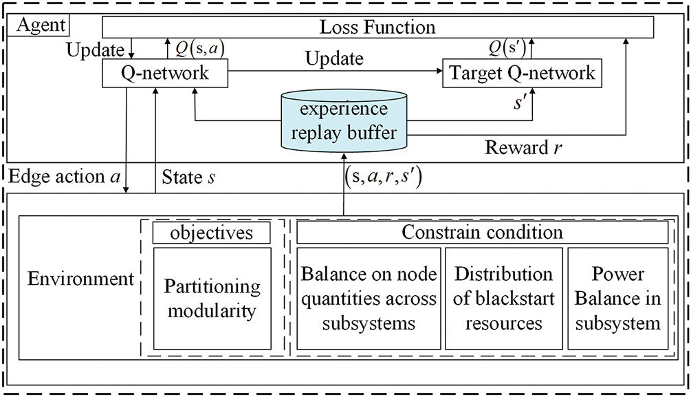
Figure 4: Process of agent-environment interaction based on DQN

As shown in Fig. 4, the agent part includes an experience replay buffer, two neural networks, and a mechanism for updating the network parameters. The environment part consists of the model’s objective and constraints. The data generated from interactions is stored in the experience replay buffer, which includes the current state s, the chosen action a, the obtained reward r, and the next state s’. After enough data accumulates in the experience replay buffer, the agent randomly samples a batch for learning. The role of Q-Network is to generate a Q-value table of actions based on the current environmental state, thereby selecting the action with the highest Q-value. The role of the Target Q-network is to enhance the stability of the Q-network’s learning process and reduce fluctuations during training. The Q-network and the target Q-network are used to compute the predicted and target Q-values, respectively. Loss function is calculated based on their difference, and the Q-network is updated using gradient descent.

4.3 Flowchart

Fig. 5 presents the flowchart of the proposed partitioning method, including 5 steps. The steps of the partitioning decision process can be simplified as follows:

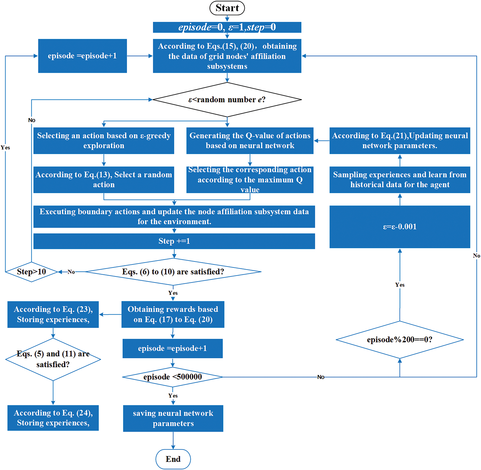
Figure 5: The flowchart of the proposed partitioning method

(1)   Initialize episode = 0, ε = 1, and obtain the data of grid nodes’ subsystem affiliations.

(2)   Generate a random number that is uniformly distributed in [0, 1]. Compare this value with ε to select either a random action or the action corresponding to the maximum Q-value.

(3)   If Eqs. (6) to (10) are satisfied, the partitioning result for the current episode is successful; otherwise, the agent continues to search for subsystem boundaries. Considering the necessity for rapid network reconfiguration following large-scale blackouts, the number of subsystem boundaries should be minimized. To meet this requirement, this paper limits the number of search actions for subsystem boundaries to Step = 10. If partitioning cannot be achieved within 10 actions for a given episode, the training is terminated for that episode and proceeds to the next episode.

(4)   After the partitioning process is completed, calculate the reward value using Eqs. (17) to (20) and store the corresponding data in the experience replay buffer defined by Eqs. (23) and (24). Furthermore, every 200 training episodes, sample data from the replay buffer to update parameters of the neural network.

(5)   Training is terminated upon reaching 50,000 episodes, and the model parameters are saved. These parameters can then be loaded into the model for online deployment, enabling the agent to generate partitioning schemes rapidly.

5  Case Studies

In this paper, a partitioning method for a power system based on DRL is implemented using Python on the PyCharm platform. The method is validated through simulation on the IEEE 39-bus test system.

Discuss the partitioning training process differences with different discount factor γ values. Compare the partitioning results of this study with those from other references to validate the effectiveness of the proposed partitioning method.

5.1 IEEE 39-Bus Test System

The IEEE 39-bus test system is shown in [40]. It consists of 10 generators, 39 buses, and 46 branches. Generators G32, G33, and G37 are designated as blackstart resources.

The hardware configuration includes a 4.05 GHz CPU, 16 GB of RAM, and an NVIDIA GeForce GT 710 GPU with 2 GB of video memory. The software configuration includes Python 3.11 and PyTorch 2.2.2. The settings for code-related parameters are shown in Table 1.

The learning rate is crucial to the model’s learning process in deep reinforcement learning. If the learning rate is too large, the model may fail to converge; if the learning rate is too small, the learning speed is slow. This paper adopts a fixed learning rate scheme, setting lr = 0.001 based on reference [31]. The more parameters about ε, εmin, and εdecrement are set based on reference [31]. According to Eq. (17), a constant α guides the agent towards higher partition quality decisions. However, the excessively large constant dominates other reward terms. Thus, the manuscript sets α = 1. Minor node deviations facilitate reasonable resource allocation. This paper sets the node-deviation threshold as Δ = 2. The reasons are as follows:

(1)   A strict zero-deviation requirement would lead to more penalties. The agent’s useful feedback from other terms would be ignored during early exploration.

(2)   Practical power grid partitioning permits minor node imbalances.

(3)   This setting provides optimization space for the DRL’s objective.

The parameters are shown in Table 1.

5.2 Analysis of Training Process and Discussion

5.2.1 The Evolution of Modularity Curves and Reward Function Curves

The variation of partitioning modularity during the training process is shown in Fig. 6.

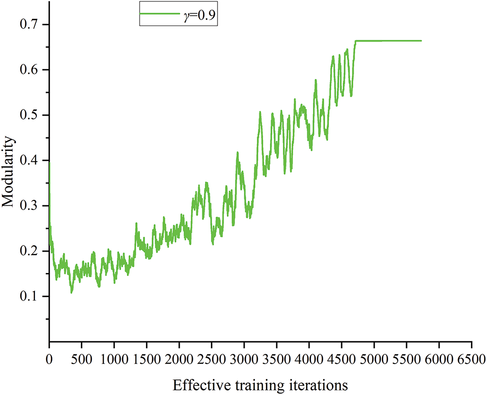
Figure 6: Modularity curve of partitioning during training

As shown in Fig. 6, in the initial stage, the partitioning result has low modularity and exhibits significant fluctuations. Due to being in a state of random exploration at this stage, random actions were given by the agent. As a result, subsystems are unreasonable. Moreover, the subsystems vary greatly among different training episodes. Therefore, modularity fluctuated significantly and remained relatively low.

As exploration experience accumulates, more data, including high-reward value data, is stored in the experience replay buffer. The agent’s policy is effectively updated through sampling from the replay buffer. The agent can give appropriate boundary actions, resulting in gradually more reasonable subsystems. Hence, the modularity curve begins to show an upward trend. The specific manifestation is the gradual increase in modularity around 1500 episodes.

Between 1500 and 2200 episodes, the curve’s rate of increase slows and exhibits steady fluctuations. This phenomenon indicates that the agent has entered the local optimization phase. At this stage, the agent can explore more reasonable partitioning results by taking actions either through random exploration or based on Q-values. Thus, the modularity curve rises further by the 2500th episode.

Between around 2500 and 3300 episodes, the boundary actions are composed of random actions and actions based on the Q-values. Therefore, subsystems vary in quality, resulting in significant fluctuations in the modularity curve. After 3300 episodes, action selection based on Q-values becomes the agent’s primary method. Thus, the boundary actions given by the agent become more fixed, resulting in a gradual decrease in fluctuations.

After multiple rounds of sampling and learning, the neural network parameters are effectively updated after 4500 episodes. The agent gives more appropriate boundary actions. Subsystems generated by the agent become more reasonable, which further increases modularity. It then converges to the maximum value around 5000 episodes.

Moreover, since the reward function integrates the modularity, node number balance, and power balance, it is necessary to analyze the convergence of all reward components. Fig. 7 shows the reward function curve during the training process of the DRL-based partitioning method.

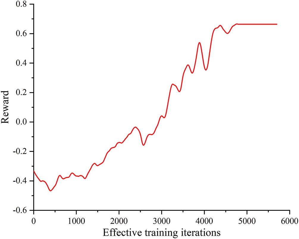
Figure 7: Reward function curve of partitioning during training

As shown in Fig. 7, as the number of training episodes increases, the reward curve gradually rises until it converges. In the first 2990 episodes, because the neural network parameters have not yet been effectively updated and random actions remain the agent’s primary choice, the partitioning result generated by the agent still fails to satisfy the relevant constraints. Primarily, during the first 1250 episodes, large penalties are incurred for constraint violations, thereby the obtained rewards are severely negative; between episodes 1250 and 2990, the reward curve begins to rise, indicating that the degree of constraint violation steadily decreases.

After episode 2990, partitioning schemes generated by the agent satisfy all constraints. Thereby, the reward curve reflects only the change of modularity. The rapid rise of the reward curve from episode 2990 to 4900 shows that the quality of generating partitioning schemes continues to improve. After episode 4900, the reward curve no longer changes. It indicates that the agent had learned to generate optimal partitioning schemes.

5.2.2 Comparison of Different Parameters

Different parameter configurations affect the performance of the agent during the training process. Discount factor γ represents the agent’s ability to predict future outcomes. A larger γ value means the agent focuses more on future rewards, demonstrating greater foresight and a broader perspective. Conversely, a smaller γ value means the agent is relatively myopic, prioritizing the immediate rewards the current action brings. Therefore, changes in the γ parameter impact the training process. Hence, the paper selects the parameter γ as a variable. The changes in the modularity of the training process are analyzed as the value of γ varies, to determine the impact of different parameter configurations on the training process. The training is conducted under three scenarios with γ values of 0.7, 0.9, and 0.99. And the modularity curves are shown in Fig. 8.

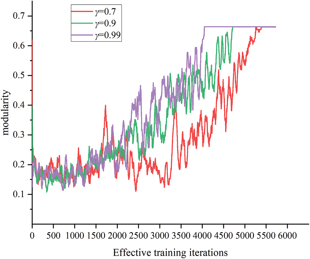
Figure 8: Modularity curves under different parameters

As shown in Fig. 8, the modularity curves under three different parameters converge to the maximum value after training. However, the curves exhibit significant differences in convergence time and fluctuation levels.

For the scenario where γ = 0.7, the relatively low value makes the agent more myopic. As a result, during the first 3500 episodes, the obtained modularity remains relatively low. The fluctuation level is becoming small, indicating that DQN training is relatively stable in this setting. However, the partitioning decision process focuses more on the rewards brought by the global results. A lower γ value means that the agent only considers the immediate reward of the current action while ignoring the impact of multiple future actions on the partitioning results. Consequently, the modularity curve exhibits the slowest convergence rate under this parameter setting.

For the scenario where γ = 0.9, the modularity curve starts to increase gradually at around 1500 episodes, and the magnitude of the increase steadily improves as training progresses. At the same time, the degree of fluctuation is also relatively small. Therefore, the value better balances the impact of current and future actions on the partitioning results.

For the scenario where γ = 0.99, the modularity increase curve is the fastest, and the convergence time is also the earliest. This is because the agent focuses more on future rewards and can consider the impact of multiple future actions on the partitioning results. However, the larger fluctuations also mean the training process is unstable and may be difficult to converge.

Therefore, considering these factors comprehensively, γ = 0.9 is more suitable for training of DQN.

5.3 Partitioning Result and Interpretation

The partitioning result provided by the agent is shown in Fig. 9.

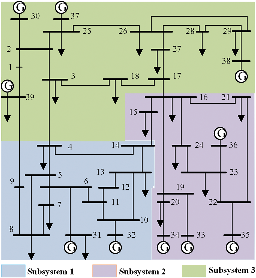
Figure 9: IEEE 39-bus test system partitioning result

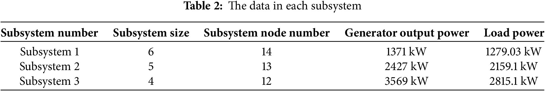
As shown in Fig. 9, edges 3-4, 14-15, 16-17, and 9-39 partition the system into three subsystems. And the relevant data for each subsystem are presented in Table 2.

Regarding the distribution of blackstart resources within the subsystems, each subsystem contains only one blackstart resource. Furthermore, each subsystem expands outward from the resource. Starting from the blackstart resource, all nodes within the subsystem can be reached through at most six branches.

Regarding the number of nodes within the subsystem, subsystem 1 has a maximum scale of 6, with 14 nodes; subsystem 2 has a maximum scale of 5, with 13 nodes; and subsystem 3 has a maximum scale of 6, with 12 nodes. Since the agent partitions the IEEE 39-bus test system into three subsystems, the average number of nodes in each subsystem is 13. Therefore, the number of nodes in the three subsystems falls within the node deviation range.

Regarding power balance within the subsystem, the generator output power of subsystem 1 is 1371 kW, while the load power is 1279.03 kW; the generator output power of subsystem 2 is 2427 kW, while the load power is 2159.1 kW; the generator output power of subsystem 3 is 3569 kW, while the load power is 2815.1 kW. Therefore, the power balance constraint for the three subsystems is met. Overall, the subsystems generated by the agent through four boundary actions have high modularity and meet all the constraint conditions. The partitioning results indicate that the agent can generate reasonable subsystems with fewer boundary actions.

5.4 Comparison and Discussion

Compare the partitioning results of the paper with those of the partitioning results in Huang et al. [6] and Lin et al. [41]. Lin et al. [41] performed partitioning for a power system based on the GN algorithm. The edges with the highest betweenness are treated as subsystem boundaries, and these boundaries are iteratively removed to achieve subsystem partitioning. The method evaluates the partitioning results using modularity and power balance within subsystems. However, the balance of subsystem sizes is not considered. The comparison is conducted based on the maximum subsystem size and modularity. The comparison results are shown in Table 3.

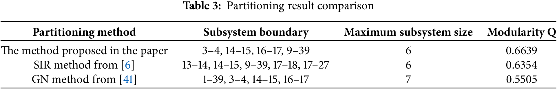
As shown in Table 3, the sizes of the three subsystems for the paper are 6, 5, and 4. Therefore, the maximum size of the subsystem is 6. And the three subsystem sizes obtained in Huang et al. [6] are 6, 6, and 6. Therefore, the maximum size of the subsystem is 6. And the three subsystem sizes obtained in Lin et al. [41] are 7, 5, and 4. Therefore, the maximum size of the subsystem is 7. The maximum size of the subsystems obtained in this paper is relatively small. Due to the balance constraint on node number among subsystems, the number of nodes in each subsystem is nearly identical, resulting in smaller subsystem sizes.

In terms of partition quality, the modularity is 0.6639 for the paper, which is greater than the modularity of the partitioning results in Huang et al. [6] and Lin et al. [41]. A higher modularity indicates better partitioning quality, with nodes within the same subsystem being more intricately connected, and fewer connections between nodes in different subsystems. Thanks to the ε-greedy strategy, the agent can explore as many partitioning results as possible, including some with high modularity. The agent generates partitioning results with higher modularity through sampling-based learning and strategy optimization.

To better visualize the differences between the three partitioning results, a radar chart was generated based on the number of subsystem boundaries, size, and the inverse of modularity, as shown in Fig. 10.

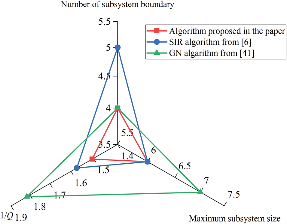
Figure 10: Modularity curves under different parameters [6,41]

Fig. 10 presents a triangular diagram with three key parameters, including the number of subsystem boundaries, subsystem size, and the inverse of modularity. Each color corresponds to a different method: red represents the proposed method in this paper, blue stands for the method from Huang et al. [6], and green indicates the approach from Lin et al. [41].

As shown in Fig. 10, a smaller triangular area indicates a more reasonable partitioning result obtained by the corresponding method. The proposed method yields the smallest triangular area, demonstrating that its partitioning results are the most optimal among the compared methods.

6  Conclusion

The partitioning decision process for the power system is formulated as an MDP. The paper proposes a novel partitioning method for a power system based on DRL. The agent can explore possible partitioning results through continuous interaction between the agent and the environment. An experience replay buffer storing high-reward actions enhances the learning efficiency of the agent. The effectiveness of this method is validated through simulation studies on the IEEE 39-bus test system. Reinforcement learning features “offline training and online deployment,” enabling the well-trained agent to generate partitioning schemes following large-scale blackouts rapidly and accurately. The partitioning scheme can serve as a reference for practical decision-making.

However, the growing number of nodes and edges in large-scale power grids elevates computational complexity and slows down the convergence speed of the proposed method. As the penetration of renewable energy continues to rise, the uncertainty of renewable energy output leads to a dynamic and uncertain operating environment, further reducing the accuracy of the proposed method. Thus, future work will focus on enhancing the convergence performance of partitioning methods for larger-scale power grid parallel restoration with high penetration of renewable energy.

Acknowledgement: Not applicable.

Funding Statement: This research was funded by the Beijing Engineering Research Center of Electric Rail Transportation.

Author Contributions: The authors confirm contribution to the paper as follows: writing—original draft preparation, Weimeng Chang; writing—review and editing, Changcheng Li, Dahai Zhang, and Jinghan He. All authors reviewed the results and approved the final version of the manuscript.

Availability of Data and Materials: The authors confirm that the data supporting the findings of this study are available within the article.

Ethics Approval: Not applicable.

Conflicts of Interest: The authors declare no conflicts of interest to report regarding the present study.

References

1. Bialek J. What does the GB power outage on 9 August 2019 tell us about the current state of decarbonized power systems? Energy Policy. 2020;146:111821. doi:10.1016/j.enpol.2020.11182. [Google Scholar] [CrossRef]

2. Stankovski J, Gjorgiev B, Locher L, Sansavini G. Power blackouts in Europe: analyses, key insights, and recommendations from empirical evidence. Joule. 2023;7(11):2468–84. doi:10.1016/j.joule.2023.09.005. [Google Scholar] [CrossRef]

3. Busby JW, Baker K, Bazilian MD, Gilbert AQ, Grubert E, Rai V, et al. Cascading risks: understanding the 2021 winter blackout in Texas. Energy Res Soc Sci. 2021;77(1):102106. doi:10.1016/j.erss.2021.102106. [Google Scholar] [CrossRef]

4. Liu Y, Fan R, Terzija V. Power system restoration: a literature review from 2006 to 2016. J Mod Power Syst Clean Energy. 2016;4(3):332–41. doi:10.1007/s40565-016-0219-2. [Google Scholar] [CrossRef]

5. Zou Y, Li H. Study on power grid partition and attack strategies based on complex networks. Front Phys. 2022;9:790218. doi:10.3389/fphy.2021.790218. [Google Scholar] [CrossRef]

6. Huang S, Ye Y, Xu W, Yang L, Luo W, Li C. A Partitioning method for parallel power system restoration based on virus propagation model. In: Proceedings of the 2020 IEEE 3rd Student Conference on Electrical Machines and Systems (SCEMS); 2020 Dec 4–6; Jinan, China. p. 369–74. doi:10.1109/SCEMS48876.2020.9352363. [Google Scholar] [CrossRef]

7. Yang C, Cheng T, Li S, Gu X. A novel partitioning method for the power grid restoration considering the support of multiple LCC-HVDC systems. Energy Rep. 2023;9(2):1104–12. doi:10.1016/j.egyr.2022.12.050. [Google Scholar] [CrossRef]

8. Yang Y, Sun Y, Wang Q, Liu Q, Zhu L. Fast power grid partition for voltage control with balanced-depth-based community detection algorithm. IEEE Trans Power Syst. 2022;37(2):1612–22. doi:10.1109/TPWRS.2021.3107847. [Google Scholar] [CrossRef]

9. Zhao C, Zhao J, Wu C, Wang X, Xue F, Lu S. Power grid partitioning based on functional community structure. IEEE Access. 2019;7:152624–34. doi:10.1109/ACCESS.2019.2948606. [Google Scholar] [CrossRef]

10. Wei X, Pan L, Xie D, Yang S, Wei S. Complex network theory and game theory-based partitioning decision-making of parallel restoration for resilient power grid. Front Energy Res. 2024;12:1343954. doi:10.3389/fenrg.2024.1343954. [Google Scholar] [CrossRef]

11. Huang S, Li C, Li Z, Xu W, Yang W. An improved label propagation algorithm-based method to develop sectionalizing strategies for parallel power system restoration. IEEE Access. 2020;8:118497–509. doi:10.1109/ACCESS.2020.3005573. [Google Scholar] [CrossRef]

12. Sun L, Sha X, Zhang S, Wang J, Yu Y. Two-stage dynamic partitioning strategy based on grid structure feature and node voltage characteristics for power systems. Energies. 2025;18(10):2544. doi:10.3390/en18102544. [Google Scholar] [CrossRef]

13. Li C, He J, Zhang P, Xu Y. A novel sectionalizing method for power system parallel restoration based on minimum spanning tree. Energies. 2017;10(7):948. doi:10.3390/en10070948. [Google Scholar] [CrossRef]

14. Ganganath N, Wang J, Xu X, Cheng C-T, Tse CKM. Agglomerative clustering-based network partitioning for parallel power system restoration. IEEE Trans Industr Inform. 2018;14(8):3325–33. doi:10.1109/TII.2017.2780167. [Google Scholar] [CrossRef]

15. Sarmadi BK, Dobakhshari AS. A parallel approach for ultra-fast state estimation in large power system using graph partitioning theory. Acta IMEKO. 2024;13(1):1–9. doi:10.21014/actaimeko.v13i1.1704. [Google Scholar] [CrossRef]

16. Hu Y, Xun P, Kang W, Zhu P, Xiong Y, Shi W. Power system zone partitioning based on transmission con-gestion identification using an improved spectral clustering algorithm. Electronics. 2021;10(17):2126. doi:10.3390/electronics10172126. [Google Scholar] [CrossRef]

17. Feng S, Cheng H, Wang Z, Zeng D. Partitioning method of reserve capacity based on spectral clustering con-sidering wind power. Int J Emerg Electric Power Syst. 2023;24(2):173–81. doi:10.1515/ijeeps-2021-0356. [Google Scholar] [CrossRef]

18. Chakrabarty M, Sarkar D, Basak R. An interactive partitioning algorithm-based electrical power crisis man-agement for service restoration with existing black-start resources considering load priority. J Inst Eng India Series B. 2021;102(2):169–78. doi:10.1007/s40031-020-00519-9. [Google Scholar] [CrossRef]

19. Kyesswa M, Murray A, Schmurr P, Çakmak H, Kühnapfel U, Hagenmeyer V. Impact of grid partitioning algorithms on combined distributed AC optimal power flow and parallel dynamic power grid simulation. IET Gener Transm Distrib. 2020;14(25):6133–41. doi:10.1049/iet-gtd.2020.1393. [Google Scholar] [CrossRef]

20. Jiang Y, Ortmeyer TH. Propagation-based network partitioning strategies for parallel power system restoration with variable renewable generation resources. IEEE Access. 2021;9(25):144965–75. doi:10.1049/iet-gtd.2020.1393. [Google Scholar] [CrossRef]

21. Wu Y, Li Q, Li Q, Chen D, Yu X, Lin J. Optimal partition for power system restoration. In: Proceedings of the 2021 IEEE 4th International Electrical and Energy Conference (CIEEC); 2021 May 28–30; Wuhan, China. p. 1–6. doi:10.1109/CIEEC50170.2021.9510697. [Google Scholar] [CrossRef]

22. Wang Z, Ding T, Mu C, Huang Y, Yang M, Yang Y, et al. An ADMM-based power system partitioned black-start and parallel restoration method considering high-penetrated renewable energy. Int J Electr Pow Energy Syst. 2024;155(1):109532. doi:10.1016/j.ijepes.2023.109532. [Google Scholar] [CrossRef]

23. Hartmann C, Zhang J, Calaza CDG, Pesch T, Michielsen K, Benigni A. Quantum annealing based power grid partitioning for parallel simulation. IEEE Trans Power Syst. 2025. doi:10.1109/TPWRS.2025.3578243. [Google Scholar] [CrossRef]

24. Li S, Lin Z, Zhang Y, Gu X, Wang H. Optimization method of skeleton network partitioning scheme considering resilience active improvement in power system restoration after typhoon passes through. Int J Elect Pow Energy Syst. 2023;148(3):109001. doi:10.1016/j.ijepes.2023.109001. [Google Scholar] [CrossRef]

25. Talib DNA, Mokhlis HB, Talip MSA, Naidu K. Islands determination for parallel power system restoration using heuristic based strategy. In: Proceedings of the 2018 IEEE Innovative Smart Grid Technologies-Asia (ISGT Asia); 2018 May 22–25; Singapore. p. 30–5. doi:10.1109/ISGT-Asia.2018.8467805. [Google Scholar] [CrossRef]

26. Sun L, Wen F, Lin Z, Xue Y, Salam MA, Ang SP, et al. Network partitioning strategy for parallel power system restoration. IET Gener Transm Distrib. 2016;10(8):1883–92. doi:10.1049/iet-gtd.2015.1082. [Google Scholar] [CrossRef]

27. Huo Y, Wang T, Wang Q, Xia F, Yin X, Li F, et al. Research on load recovery optimization strategy based on power grid partition. IOP Conf Ser Earth Environ Sci. 2019;300(4):042111. doi:10.1088/1755-1315/300/4/042111. [Google Scholar] [CrossRef]

28. Pan ZJ, Zhang Y. A flexible black-start network partitioning strategy considering subsystem recovery time balance. Int Trans Electr Energ Syst. 2014;25(8):1644–56. doi:10.1002/etep.1932. [Google Scholar] [CrossRef]

29. Du Y, Wu D. Deep reinforcement learning from demonstrations to assist service restoration in islanded microgrids. IEEE Trans Sustain Energy. 2022;13(2):1062–72. doi:10.1109/TSTE.2022.3148236. [Google Scholar] [CrossRef]

30. Hosseini MM, Rodriguez-Garcia L, Parvania M. Hierarchical combination of deep reinforcement learning and quadratic programming for distribution system restoration. IEEE Trans Sustain Energy. 2023;14(2):1088–98. doi:10.1109/TSTE.2023.3245090. [Google Scholar] [CrossRef]

31. Igder MA, Liang X. Service restoration using deep reinforcement learning and dynamic microgrid formation in distribution networks. IEEE Trans Ind Appl. 2023;59(5):5453–72. doi:10.1109/TIA.2023.3287944. [Google Scholar] [CrossRef]

32. Newman MEJ, Girvan M. Finding and evaluating community structure in networks. Phys Rev E. 2004;69(2):026113. doi:10.1103/PhysRevE.69.026113. [Google Scholar] [PubMed] [CrossRef]

33. Clauset A, Newman MEJ, Moore C. Finding community structure in very large networks. Phy Rev E. 2004;70(6 Pt 2):066111. doi:10.1103/PhysRevE.70.066111. [Google Scholar] [PubMed] [CrossRef]

34. Chen B, Ye Z, Chen C, Wang J. Toward a MILP modeling framework for distribution system restoration. IEEE Trans Power Syst. 2019;34(3):1749–60. doi:10.1109/TPWRS.2018.2885322. [Google Scholar] [CrossRef]

35. Zhao J, Liang Y, Fang Y, Weng Y, Ma W, Zhang M, et al. Multiple black-start power supplies planning scheme considering partition recovery. Electr Power Syst Res. 2023;215:109006. doi:10.1016/j.epsr.2022.109006. [Google Scholar] [CrossRef]

36. Foraboschi P. Suggestions for a new epistemology of structural engineering. In: Vesper: vesper no. 8. Macerata, Italy: Quodlibet; 2023. p. 154–68. doi:10.2307/jj.4688086.16. [Google Scholar] [CrossRef]

37. Verma PR, Singh NP, Pantola D, Cheng X. Neural network developments: a detailed survey from static to dynamic models. Comput Electr Eng. 2024;120(1):109710. doi:10.1016/j.compeleceng.2024.109710. [Google Scholar] [CrossRef]

38. Mnih V, Kavukcuoglu K, Silver D, Rusu AA, Veness J, Bellemare MG, et al. Human-level control through deep reinforcement learning. Nature. 2015;518(7540):529–33. doi:10.1016/j.compeleceng.2024.109710. [Google Scholar] [CrossRef]

39. Ji Y, Le W, Tian X, Liu G, Han L, Cui T. Double replay buffer mechanism for deep reinforcement learning algorithm. In: Proceedings of the 2024 4th International Conference on Electronic Information Engineering and Computer Science (EIECS); 2024 Sep 27–29; Yanji, China. p. 870–3. doi:10.1109/EIECS63941.2024.10800212. [Google Scholar] [CrossRef]

40. Liu F, Gu B, Qin S, Zhang K, Cui L, Xie G. Power grid partition with improved biogeography-based optimization algorithm. Sustain Energy Technol Assess. 2021;46(1):101267. doi:10.1016/j.seta.2021.101267. [Google Scholar] [CrossRef]

41. Lin ZZ, Wen FS, Chung CY, Wong KP, Zhou H. Division algorithm and interconnection strategy of restoration subsystems based on complex network theory. IET Gener Transm Distrib. 2011;5(6):674–83. doi:10.1049/iet-gtd.2010.0586. [Google Scholar] [CrossRef]