
 Submit a Paper
 Propose a Special lssue
 Open Access
ARTICLE
Research on Electric Vehicle Charging Optimization Strategy Based on Improved Crossformer for Carbon Emission Factor Prediction
1 Marketing Service Center of State Grid Jibei Electric Power Co, Ltd., Xicheng District, Beijing, 100051, China
2 School of Electrical and Electronic Engineering, North China Electric Power University, Changping District, Beijing, 102206, China
* Corresponding Author: Zixuan Meng. Email:
(This article belongs to the Special Issue: Artificial Intelligence-Driven Collaborative Optimization of Electric Vehicle, Charging Station and Grid: Challenges and Opportunities)
Energy Engineering 2026, 123(1), 15 https://doi.org/10.32604/ee.2025.069576
Received 26 June 2025; Accepted 13 October 2025; Issue published 27 December 2025
 View Full Text
 Download PDF
Abstract
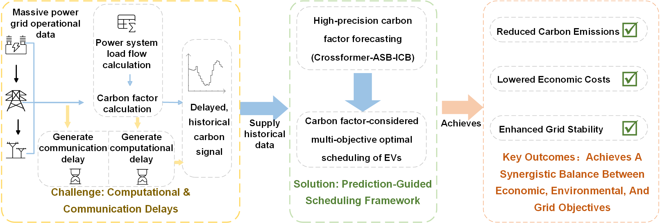
To achieve low-carbon regulation of electric vehicle (EV) charging loads under the “dual carbon” goals, this paper proposes a coordinated scheduling strategy that integrates dynamic carbon factor prediction and multi-objective optimization. First, a dual-convolution enhanced improved Crossformer prediction model is constructed, which employs parallel 1 × 1 global and 3 × 3 local convolution modules (Integrated Convolution Block, ICB) for multi-scale feature extraction, combined with an Adaptive Spectral Block (ASB) to enhance time-series fluctuation modeling. Based on high-precision predictions, a carbon-electricity cost joint optimization model is further designed to balance economic, environmental, and grid-friendly objectives. The model’s superiority was validated through a case study using real-world data from a renewable-heavy grid. Simulation results show that the proposed multi-objective strategy demonstrated a superior balance compared to baseline and benchmark models, achieving a 15.8% reduction in carbon emissions and a 5.2% reduction in economic costs, while still providing a substantial 22.2% reduction in the peak-valley difference. Its balanced performance significantly outperformed both a single-objective strategy and a state-of-the-art Model Predictive Control (MPC) benchmark, highlighting the advantage of a global optimization approach. This study provides theoretical and technical pathways for dynamic carbon factor-driven EV charging optimization.Graphic Abstract
Keywords
The global transition towards carbon neutrality imposes stringent requirements on the low-carbon transformation of energy and power systems [1,2]. A critical challenge in this transition is the accurate accounting of carbon emissions across the entire power chain (generation, grid, and consumption), particularly given their significant spatio-temporal dynamics [3,4]. The introduction of the concept of consumption-based carbon accounting (embodied emissions or indirect carbon responsibility) establishes a critical link between carbon emissions and end-use consumption behavior [5]. This paradigm shift offers a fundamentally new perspective for measuring and attributing carbon emissions [6,7]. For instance, while consumers purchasing goods do not directly emit carbon, the production of those goods entails emissions; these embodied emissions constitute the indirect carbon responsibility associated with the purchase. Electric vehicles (EVs), as crucial flexible loads in modern power systems [8], exhibit substantial spatio-temporal heterogeneity in their embodied carbon emissions during charging [9]. Accurately quantifying these dynamic emissions is thus a key prerequisite for realizing effective carbon-aware charging regulation [10].
Current research on EV charging typically uses static, grid-average carbon factors for indirect carbon accounting [11,12]. This approach fails to capture the dynamic carbon intensity introduced by high penetrations of variable renewable energy and strong source-load fluctuations [13]. Implementing truly carbon-aware charging optimization necessitates the introduction of carbon emission factors with much finer temporal granularity [14].
While physics-based carbon flow tracing methods can theoretically provide this data [15–17], their dependence on complete grid data makes them vulnerable to communication delays and data deficiencies [18,19]. Consequently, data-driven methods, particularly deep learning, have emerged as a promising alternative for forecasting nodal carbon factors [20,21]. The evolution of Transformer-based architectures highlights the ongoing challenge of modeling complex time series. While early models like Informer focused on improving computational efficiency for long sequences [22], subsequent approaches such as NSTransformer specifically targeted non-stationarity by decoupling the series into trend and variation components [23]. More recent models like iTransformer and Crossformer have further advanced performance by exploring inverted channel-wise attention and 2D array processing, respectively [24,25], while their focus remains on general time-series representation, lacking functionality for adaptive denoising and fine-grained local pattern extraction.
A significant body of research has focused on the strategic optimization of EV charging. The work by Sahoo and Sivasubramani for instance, first proposes a Particle Swarm Optimization (PSO) based charging coordination strategy for industrial PEV fleets with the integration of solar and wind energy [26], and later extends this into a comprehensive framework that also includes strategic charging station placement [27]. However, both studies are limited to single-objective cost minimization and do not explicitly incorporate grid-friendliness or carbon emissions as optimization objectives. Addressing the need for trade-offs, Yan et al. introduce a multi-objective strategy using an entropy weight method to balance grid load variance against EV owner costs, yet this approach still omits carbon emissions as a key objective [28]. Further expanding the scope, Ahmadi et al. present a stochastic multi-objective framework that co-optimizes for both economic costs and carbon emissions under system uncertainties [29]; however, its environmental dispatch lacks fine-grained precision as it relies on static, non-time-varying carbon emission factors. In parallel with these frameworks, other research has explored facets such as the evaluation of charging load flexibility [30], price-driven load shifting [31,32], and cluster modeling considering charging behavior [33]. However, these advanced scheduling strategies often operate under the assumption of a static or simplified carbon landscape. A critical research gap remains in developing optimization frameworks that are natively guided by high-fidelity, forward-looking carbon signals to unlock deeper emission reduction potential without compromising grid and economic objectives.
This paper addresses this gap by proposing a novel framework that synergistically combines prediction and optimization. We first introduce Crossformer-ASB-ICB, an enhanced Crossformer architecture that integrates an Adaptive Spectral Denoising Block (ASB) and a novel Integrated Convolution Block (ICB) to significantly improve the prediction accuracy for highly volatile carbon emission factor sequences. Building on these high-precision forecasts, we then propose a carbon factor prediction-guided multi-objective EV charging optimization strategy. By formulating a carbon-electricity cost joint optimization model, it provides a practical pathway for realizing fine-grained, low-carbon regulation of EV charging loads in support of carbon neutrality goals.
2 Improved Crossformer Model for Carbon Emission Factor Prediction
2.1 Crossformer Model Basic Architecture
Crossformer is an improved Transformer architecture. Compared to previous Transformer architectures, its core innovations lie in: data segmentation transforming the input sequence into a two-dimensional vector array; subsequently, employing a Two-Stage Attention (TSA) layer to efficiently capture both cross-variable and cross-time dependencies; and finally, adopting a hierarchical encoder-decoder structure to leverage information at different levels (scales) for prediction.
(1) Data Segmentation
The attention values in the original Transformer, when applied to time series forecasting, inherently tend to be segmented, meaning proximate data points exhibit similar attention weights. The Dimension-Segment-Wise (DSW) embedding method addresses this by dividing the points of each dimension into segments of length L before embedding:
The embedded input is
where
(2) Two-Stage Attention Mechanism
For each dimension, the Multi-head Self-Attention (MSA) mechanism is directly applied to capture dependencies between different time segments within the same dimension. The computational complexity is
Applying MSA directly between different dimensions would lead to a complexity of
(3) Hierarchical Encoder-Decoder Structure
The encoder merges adjacent segments within the same dimension, obtaining a coarser-grained representation:
The decoder receives N + 1 feature arrays from the encoder output and, by combining self-attention and cross-attention mechanisms, achieves multi-dimensional feature fusion and establishes connections between the encoder and decoder.
2.2 Improved Crossformer Model
This paper enhances the Crossformer architecture by integrating an Adaptive Spectral Block (ASB) and an Interactive Convolutional Block (ICB). The ASB adaptively processes the signal in the frequency domain to mitigate noise, while the ICB uses parallel 1D convolutions to extract multi-scale local features. Fig. 1 illustrates how the ASB and ICB modules are integrated into the Crossformer architecture.
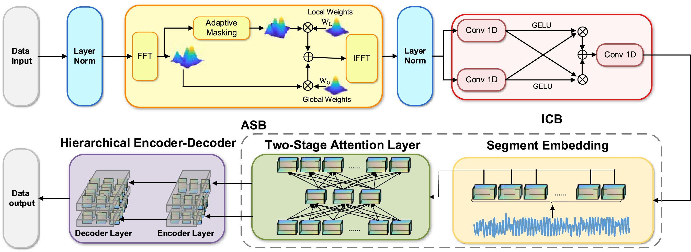
Figure 1: Architecture of the proposed crossformer model with integrated ICB and ASB modules
The Adaptive Spectral Block (ASB) utilizes frequency-domain processing for robust feature extraction. The ASB first applies a Fast Fourier Transform (FFT) to the time-domain input to obtain its frequency-domain representation, F. The module then employs two sets of learnable parameters, optimized during training to minimize the final task loss: a quantile parameter,
The noise mitigation is performed via a dynamic masking process based on the signal’s energy spectrum. The learned parameter θ determines a relative cut-off point to create a binary mask, producing a denoised representation,
Subsequently, the learnable filters are applied in a dual-pathway structure. The ‘global filter’
According to the Convolution Theorem, this element-wise multiplication in the frequency domain is mathematically equivalent to performing a circular convolution in the time domain. The frequency-domain filtering enables large-scale feature learning at low computational cost. Finally, an Inverse Fast Fourier Transform (IFFT) transforms the integrated representation back into the time domain.
The Interactive Convolutional Block (ICB) then employs two parallel 1D convolutional paths to process the signal. The first path uses a kernel of size 1 for efficient, pointwise feature transformation. The second path uses a kernel of size 3 to capture local dependencies. We selected a kernel of size 3 because it effectively balances pattern capture with computational cost, and its odd size ensures proper temporal alignment.
After a GELU activation (
here, X is the input tensor,
3 Multi-Objective Electric Vehicle Charging Optimization Strategy Based on an Improved Crossformer
Building on the high-precision prediction model, this study explores dynamic integration of these predictions into EV charging scheduling strategies. In practical operations, inherent trade-offs exist among user economic demands, grid load peak-valley difference constraints, and carbon reduction targets. To address this, we propose a dynamic carbon signal-incorporated multi-objective optimization model with the following core objectives:
(1) Grid-Friendliness: Smooth load fluctuations and reduce peak-valley differences.
(2) Economic Efficiency: Minimize user charging costs (considering time-of-use electricity prices and battery degradation).
(3) Carbon-Awareness: Dynamically identify low-carbon charging periods using predicted carbon factors.
Through a tri-objective collaborative optimization mechanism, we achieve balanced decision-making considering the interests of users, grid operators, and environmental sustainability.
3.1 V2G-Capable EV Charging/Discharging Model
Dispatchable EVs are categorized into two groups: those supporting bidirectional discharge (Vehicle-to-Grid, V2G) and non-V2G-capable vehicles.
here,
Due to the influence of charging and discharging efficiency
This is the battery State-of-Charge (SOC) update formula.
SOC Constraints:
3.2 Charging and Discharging Optimization Objective Function
Our optimization strategy includes the following objectives:
(1) To comprehensively consider load fluctuation and peak-to-valley difference.
(2) Time-of-use electricity price cost and electric vehicle battery degradation cost.
(3) Carbon emissions
(4) Single-objective transformation of multi-objective optimization
The conversion of the multi-objective problem into the single-objective function
Secondly, the selection of the weighting coefficients (
4.1 Experimental Parameter Settings
(1) Carbon Factor and Crossformer Configuration
The carbon factor dataset used in this study was synthesized to reflect the operational characteristics of a typical regional power grid with a high penetration of renewable energy, with its key parameters informed by actual data from the North China grid. The generation process adhered to physical constraints. First, a baseline trend and boundary conditions were established by analyzing the typical daily load curves, generation mix, and the output characteristics of major power plants representative of such a grid. This determined the carbon factor’s range and trend, which are governed by the time-varying renewable energy penetration. Subsequently, stochastic fluctuations were introduced upon this high-fidelity baseline to simulate uncertainties, such as the integration of distributed renewable energy. This methodology resulted in a semi-simulated dataset that preserves the macroscopic dynamics of a real-world system while providing the necessary scale for deep learning-based research. The carbon factor is defined as:
For the model architecture, based on the 15-min sampling frequency of the data, the input window length was set to 96 to ensure the capture of a full 24-h diurnal cycle. The segment length required by the Crossformer architecture was set to 12. The model’s core dimension was 64, configured with 8 attention heads, 2 encoder layers, and 1 decoder layer. This configuration was chosen to balance the model’s capacity for learning complex patterns against computational overhead. During the training phase, the Adam optimizer was employed with a batch size of 64. The initial learning rate was set to 0.0001, a standard and empirically effective value that generally ensures stable convergence for Transformer-based models. To prevent overfitting, an early stopping mechanism was utilized with a patience of 20% of the total epochs. The dataset was divided into training and testing sets with an 80/20 ratio after Min-Max scaling.
here, x is a value in the original data;
To further validate the rationale behind our key hyperparameter choices, a sensitivity analysis was conducted, focusing on the impact of the input window length (tested over the range {24, 48, 96, 144}) and the learning rate (tested over the range {0.01, 0.001, 0.0001, 0.00001}). The detailed results of this analysis are presented in the Experimental Results section.
To systematically evaluate the effectiveness of the Interactive Convolution Block (ICB) and the Adaptive Spectral Block (ASB) proposed in this study, we designed a comprehensive ablation study. This study aims to quantify the individual contributions of each module, their synergistic effects, and the impact of their sequential order. We compared the following five model variants: (1) the Backbone model, which is the original Crossformer; (2) the model with only ICB integrated (+ICB); (3) the model with only ASB integrated (+ASB); (4) the model with ICB integrated before ASB (+ICB → ASB); and (5) the model with ASB integrated before ICB (+ASB → ICB). All variants were evaluated across multiple forecast horizons, including short-term (15-min), mid-term (1, 2, 3-h), and long-term (6, 12-h) predictions.
In the experimental results analysis, R2 (coefficient of determination) and MAPE (Mean Absolute Percentage Error) are selected as core metrics to evaluate the model’s prediction performance, while MAE (Mean Absolute Error) serves as an auxiliary metric.
here,
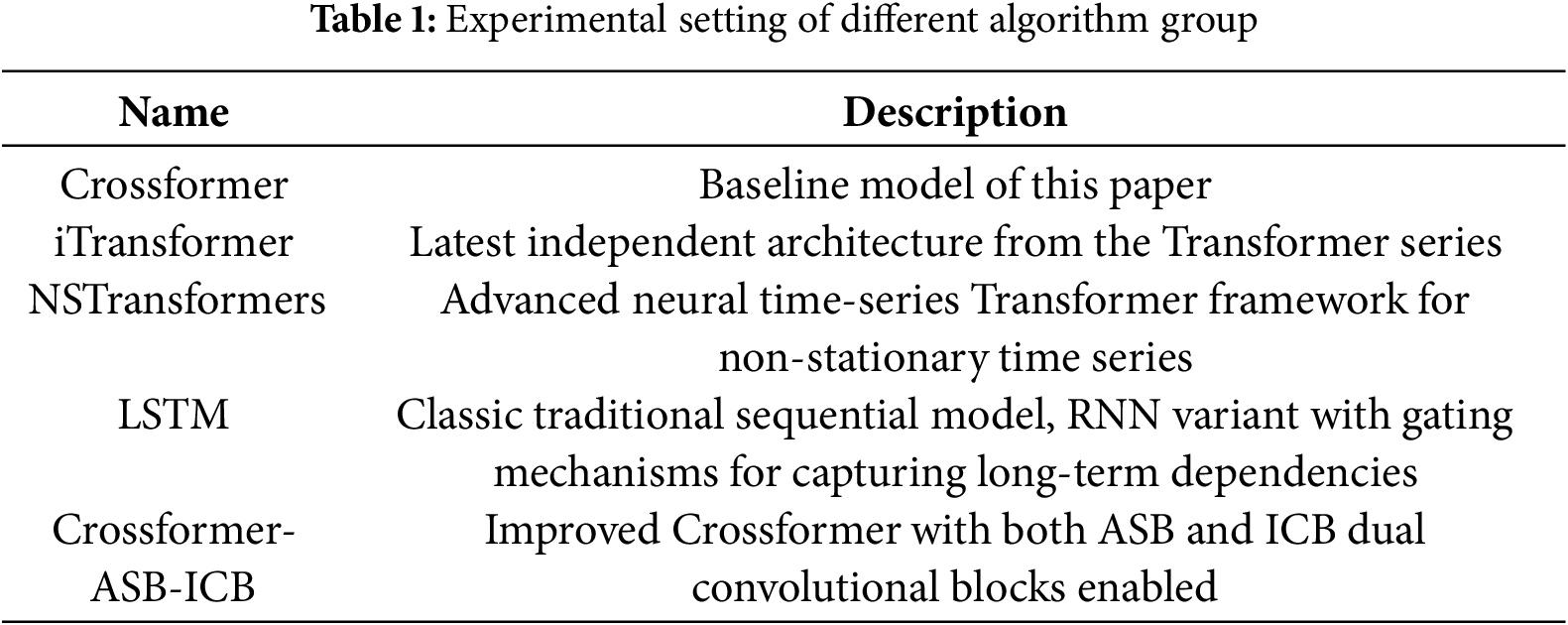
Crossformer is selected as the baseline model, and the more advanced iTransformer and NSTransformers from the Transformer series are used as control groups for the model experiments. The specific control groups used in the experiments are detailed in Table 1.
(2) Electric Vehicle Parameter Configuration
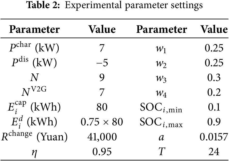
The multi-objective optimization experiment is based on a typical daily load curve of a certain building, with 9 electric vehicles selected for scheduling, of which 7 support V2G charging and discharging, and 2 are conventional vehicles that only charge. Experimental parameters are shown in Table 2, and the simulation period is 24 h.
(1) Initial Energy Generation
To simulate diverse user behavior, initial energy
(2) Grid Connection Period Generation
here,
(3) Baseline Scenario Construction
In scenarios without optimization, vehicles continuously charge at maximum power
here,
(4) Experimental Setup and Optimization Scenarios
To comprehensively evaluate the performance and scalability of the proposed multi-objective strategy under varying scales and complexities, two progressive case studies were designed and simulated using the CPLEX solver.
Case Study 1: Detailed Analysis of a Dispatchable Fleet at the Charging Station Level
This case study focuses on a fully dispatchable fleet of electric vehicles within a charging station. The primary objective is to conduct a detailed performance analysis of the model and to thoroughly investigate the intrinsic trade-offs among the different optimization objectives (grid load fluctuation, peak-to-valley difference, economic cost, and carbon emissions). The following optimization scenarios are compared:
Unoptimized Charging (Baseline): Simulates EVs charging immediately at maximum power upon connection.
Control Group: Minimizing peak-to-valley difference as the single objective:
Experimental Group: With a weighted comprehensive objective:
To thoroughly investigate the intrinsic trade-offs between competing optimization objectives, a Pareto front analysis was conducted within this case study. The analysis focused on the core conflicting objectives of economic cost (
The specific parameters for this case are detailed in Table 2.
Case Study 2: Scalability and Realism Simulation of a Regional Fleet
To validate the applicability of the proposed strategy in larger and more realistic scenarios, a second case study was designed. This case simulates a medium-sized charging station or a regional fleet with a daily traffic of approximately 100 vehicles. In this scenario, it is assumed that 20% of the fleet (i.e., 20 vehicles) agrees to participate in the optimized dispatching program, while the remaining 80% follow uncontrolled charging patterns.
To reflect fleet diversity, the 20 participating vehicles are composed of 7 V2G-capable vehicles (capable of bidirectional charging and discharging) and 13 vehicles capable of orderly charging only (i.e., shifting charging times without discharging). The objective of this case study is to validate the performance, robustness, and scalability of the proposed multi-objective strategy when faced with a large, uncontrollable background load and a diverse dispatchable fleet.
4.2 Experimental Results and Analysis
4.2.1 Carbon Factor Prediction Model Evaluation
Comparative Analysis with Baseline Models
To validate the effectiveness of the model proposed in this study, we conducted a comparative analysis against several baseline models, including the original Crossformer, two advanced Transformer variants (iTransformer, NSTransformers), the hybrid CNN-GRU model, and the classic LSTM model. First, for the task of single-step (15-min) ultra-short-term forecasting, the detailed performance comparison is presented in Table 3.
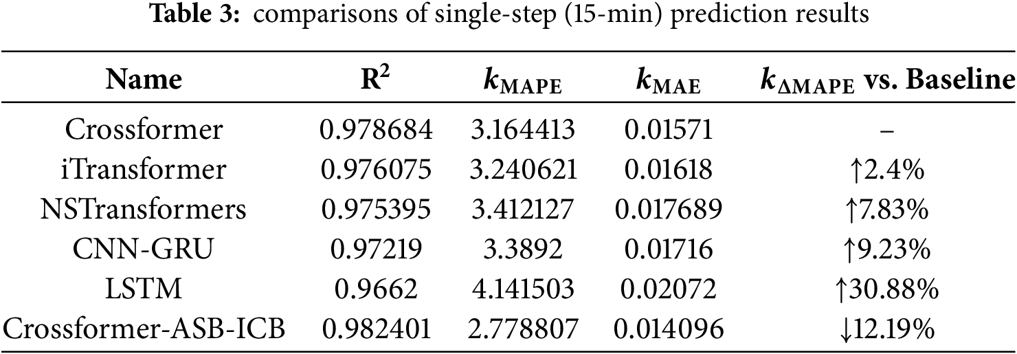
It is evident from the table that the proposed Crossformer-ASB-ICB model achieves superior performance across all evaluated metrics. Specifically, it records the highest R2 of 0.9824, the lowest MAPE of 2.7788%, and the lowest MAE of 0.0141. Compared to the original Crossformer baseline, our model reduces the MAPE by a significant 12.19%. It is also noteworthy that the other baseline models, including iTransformer, NSTransformers, CNN-GRU, and LSTM, failed to outperform the original Crossformer in this task, which further underscores the effectiveness of our proposed ICB and ASB modules in extracting transient features.
To further assess the model’s robustness in mid-to-short-term forecasting, we extended the comparison to multiple forecast horizons of 1, 2, and 3 h, with the results shown in Table 4.
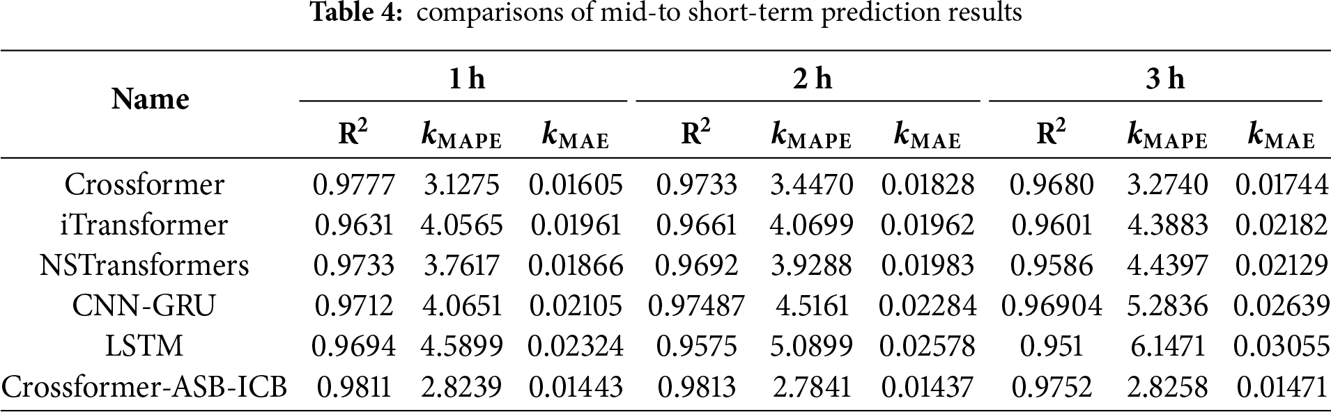
The Crossformer-ASB-ICB model consistently and comprehensively outperforms all baseline models across all horizons. A more critical observation is that the performance advantage of our proposed model becomes more pronounced as the prediction length increases. For instance, the absolute reduction in MAPE compared to the Crossformer baseline grows from 0.36 at the 1-h horizon to 1.11 at the 3-h horizon. This trend strongly demonstrates that the synergistic effect of the ICB and ASB modules is particularly effective for capturing the more complex temporal dependencies required for longer-range forecasting, thereby validating the superiority of our feature enhancement architecture design.
Fig. 2 visualizes the MAPE results from Tables 3 and 4 to provide a comparative analysis of model performance stability across increasing prediction horizons. As illustrated by the trend lines, the prediction error for all models increases as the forecast horizon extends. However, the proposed Crossformer-ASB-ICB model exhibits a demonstrably flatter error curve compared to the baseline models. This observation indicates that our proposed architecture is more robust against error accumulation, showing greater performance stability, particularly in mid-to-long-term forecasting.
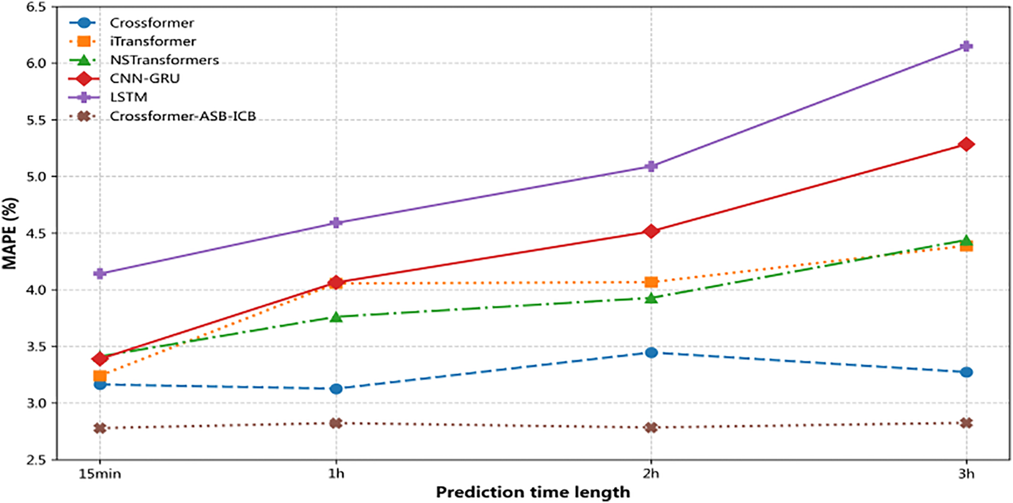
Figure 2:
Ablation Study
To systematically quantify the contribution of each proposed module, an ablation study was conducted, with the detailed results presented in Table 5.
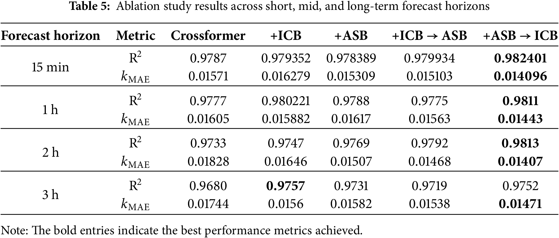
The analysis of Table 5 leads to the following conclusions: First, the individual integration of either the ICB or the ASB module yields tangible, albeit varied, performance improvements over the baseline Crossformer. Specifically, the ASB module shows a notable impact on reducing MAE in ultra-short-term forecasting (15 min), whereas the ICB module demonstrates its advantages more consistently by improving the R2 score in mid-term horizons (1–3 h).
Furthermore, a clear synergistic effect is observed when both modules are combined, outperforming the single-module variants. Notably, the sequential order of these modules is critical. The +ASB → ICB configuration achieves consistently superior performance across nearly all scenarios, maintaining the lowest Mean Absolute Error (MAE) across all forecast horizons. This result indicates that pre-processing the input sequence with the ASB before the ICB performs local feature extraction in the time domain is the optimal architectural choice for this study.
Hyperparameter Sensitivity Analysis
To further validate the rationality and robustness of our key hyperparameter selections, we conducted a comprehensive sensitivity analysis, with the results summarized in Tables 6 and 7. This study individually varied five key parameters—the learning rate, input window length, ICB kernel size, number of attention heads, and segment length—while holding all other parameters constant at their determined optimal values (highlighted in bold).
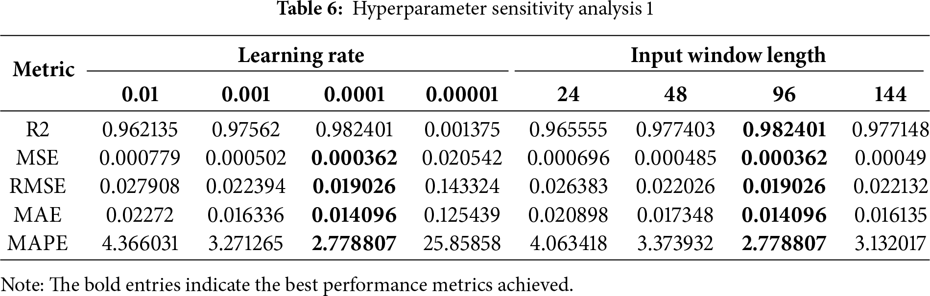
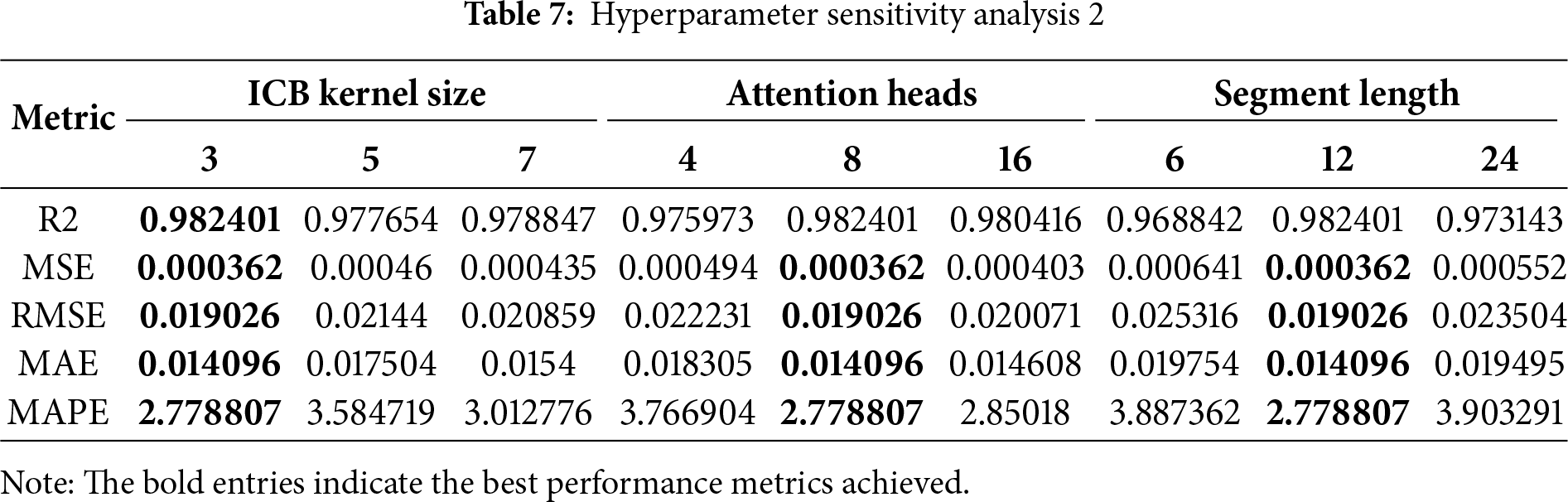
The analysis clearly demonstrates the model’s sensitivity to these hyperparameter choices. For the learning rate, performance peaks at our baseline value of 0.0001, as higher rates lead to unstable convergence while a lower rate is insufficient for effective learning. Similarly, for the input window length, performance improves as the length increases from 24 to our chosen baseline of 96 but slightly degrades at 144 steps, confirming that 96 is the optimal choice for capturing the full 24-h cycle. Regarding the ICB kernel size and segment length, the results also show a clear peak in performance at our baseline selections of 3 and 12, respectively. Finally, the analysis of the number of attention heads confirmed that our baseline configuration of 8 heads provides the best and most stable performance, validating our selection. Overall, this analysis demonstrates that our selected set of hyperparameters is robust and represents an effective configuration for the task at hand.
4.2.2 EV Charging Optimization Strategy Evaluation
To comprehensively validate the proposed model, this section presents two distinct case studies. The first case focuses on a detailed analysis of a schedulable fleet at the charging station level, while the second case evaluates the model’s performance and scalability using real-world grid data.
Case Study One: Charging Station-Level Schedulable Fleet Analysis
This section provides a detailed evaluation of the simulation results for Case Study One. The analysis will first examine the State of Charge (SOC) trajectories of the EVs to verify the fundamental dispatch logic. Subsequently, a comparative analysis of load curves and Key Performance Indicators (KPIs) will be conducted to quantify the superiority of the multi-objective strategy over the baseline and single-objective scenarios. Finally, a Pareto front analysis will be presented to thoroughly investigate the intrinsic trade-offs among the different objectives.
Fig. 3 employs a dual-axis design to visually represent the spatio-temporal coupling relationship between V2G EV SOC evolution and time-of-use electricity prices under the multi-objective optimization.

Figure 3: Spatiotemporal coupling relationship between SOC and time-of-use pricing in multi-objective optimization
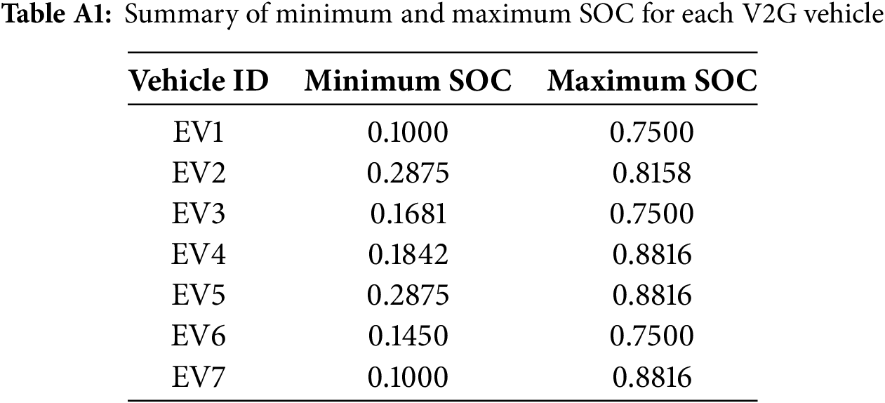
From the figure, it is evident that the SOC lower limit is 0.1 and the upper limit is 0.9. This adherence is guaranteed by the model’s design, as the SOC limits are implemented as hard constraints. Any feasible solution generated by the CPLEX solver must, by definition, strictly satisfy these bounds. To provide explicit numerical validation, a summary of the minimum and maximum SOC values for each vehicle is detailed in Table A1 in Appendix A.1, which quantitatively confirms that all trajectories remain within the prescribed operational range. Upon leaving the grid, all vehicles met the required departure energy of
Figs. 4 and 5 respectively provide a visual and quantitative comparison of the optimization effects under different strategies.

Figure 4: Load curve comparison
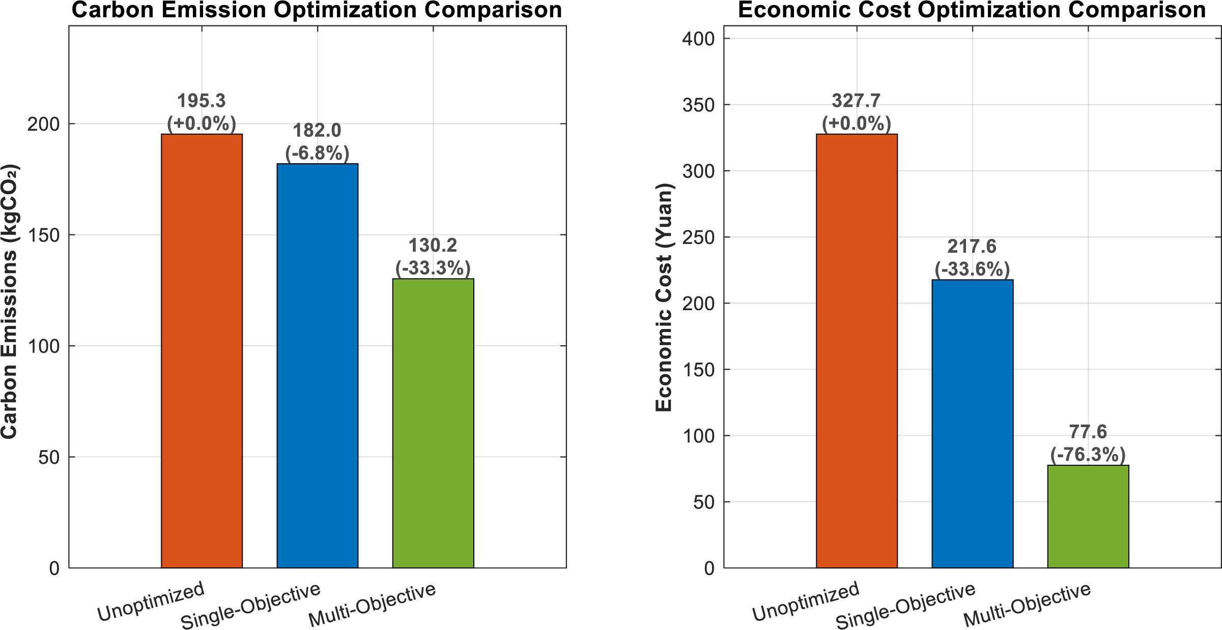
Figure 5: Optimization effect comparison chart
As shown in Fig. 4, the base load has a peak-to-valley difference of 150 kW. In the unoptimized scenario (red dashed line), the charging load overlaps with the base load’s peak hours, significantly exacerbating the grid’s peak-valley conflict. The Single-Objective strategy (blue dashed line), solely focused on minimizing this difference, successfully reduces the peak-valley difference to 87 kW (a 42% reduction). However, its dispatch behavior is suboptimal, as it still exhibits unnecessary charging peaks during high-cost, high-carbon periods in the evening, failing to fully leverage the flexibility of the EVs.
This observation is quantitatively confirmed by the results in Fig. 5. The single-objective optimization yields limited improvements in economic and environmental benefits, with only a 33.6% reduction in cost and a 6.5% reduction in carbon emissions. In contrast, the Multi-Objective approach (green solid line) demonstrates superior co-optimization capabilities. While achieving the same level of peak-valley control (also 87 kW, a 42% reduction), it intelligently co-ordinates dispatch based on both electricity prices and carbon factors. This results in a 33.4% reduction in carbon emissions (from 195.5 to 130.2 kgCO2) and a remarkable 76.3% reduction in economic costs (from 327.7 to 77.6 Yuan), achieving a high degree of synergy between grid-friendliness, economy, and environmental protection.
To further investigate the intrinsic trade-offs between economic and environmental objectives and to validate the rationality of the selected weights, a Pareto front analysis was conducted.
As illustrated in Fig. 6, the frontier clearly exhibits the substitution effect between cost and carbon reduction: pursuing lower carbon emissions inevitably comes at a higher economic cost. The solution corresponding to our baseline weights (indicated by the red star) is located on this efficient frontier. This point achieves a substantial cost reduction while also considering significant carbon emission benefits, demonstrating the rationality and superiority of the chosen weight configuration in multi-objective decision-making and validating the effectiveness of the collaborative dispatch method.
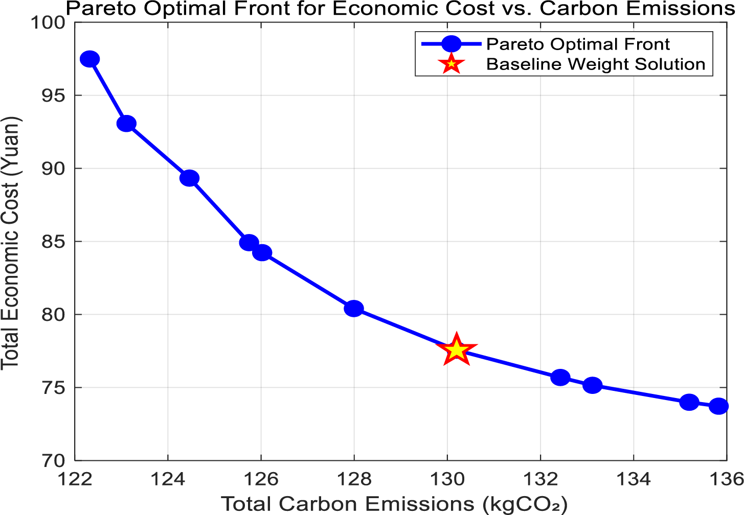
Figure 6: Pareto optimal front for economic cost vs. carbon emissions
Case Study Two: Validation with Real-World Data and SOTA Comparison
The simulation results provide a clear and quantitative comparison of the four strategies: Unoptimized, Single-Objective (Peak-Valley Minimization), the proposed Multi-Objective model, and the MPC benchmark. The overall performance is summarized in the Key Performance Indicator (KPI) comparison chart in Fig. 7.
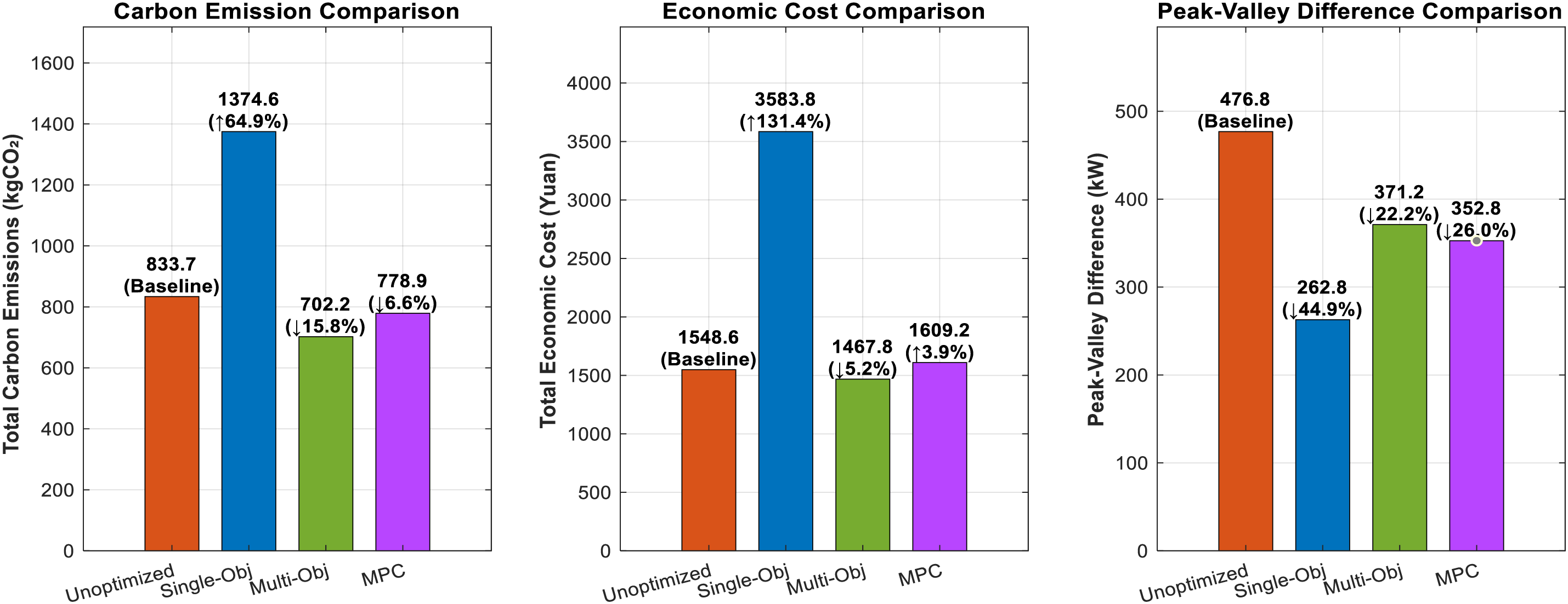
Figure 7: Comparative analysis of key performance indicators (KPIs) for different optimization strategies
The results presented in Fig. 7 are highly conclusive and reveal the unique challenges of optimization in a grid with high renewable penetration. It is noteworthy that the real-world EV load in this region already shows a tendency for users to self-charge during the midday low-cost, low-carbon period. When this EV load is superimposed on the typical urban background net load, it creates a significant “load valley” for the grid. Under this specific simulation scenario, strategies that pursue grid-friendliness (i.e., valley-filling) may conflict to some extent with economic and environmental objectives, as this requires shifting some charging activities out of the optimal midday period.
The Single-Objective strategy perfectly illustrates this conflict: while it was the most effective at peak shaving (reducing the peak-valley difference by 44.9%), it proved to be economically and environmentally untenable. By forcing charging load out of the optimal midday window to fill the valley, it caused a staggering 131.4% increase in economic cost and a 64.9% increase in carbon emissions compared to the unoptimized baseline. This confirms that a singular focus on grid flatness is impractical in such real-world scenarios.
The MPC benchmark demonstrated a moderate capability for carbon reduction (−6.6%) and effective peak-shaving (−26.0%). However, it failed to achieve economic savings, resulting in a slight cost increase of 3.9%. This suggests that while MPC is a potent real-time control tool, its inherent “short-sightedness” due to the rolling horizon can limit its ability to find globally cost-optimal schedules in a complex price and grid environment.
In stark contrast, the proposed Multi-Objective model emerged as the unequivocally superior strategy by finding an excellent balance within this complex trade-off. It was the only approach to successfully achieve simultaneous improvements across all three key domains. It delivered the highest carbon reduction at 15.8%, was the only method to achieve a significant cost reduction at −5.2%, and still provided a substantial peak-valley difference reduction of 22.2%. This balanced performance highlights the key advantage of the global optimization approach: its perfect foresight over the 24-h dispatch period allows it to identify and exploit the globally optimal trade-offs between grid stability, economic cost, and carbon emissions.
To understand the dispatch behavior that leads to these outcomes, Fig. 8 illustrates the aggregated load profiles.
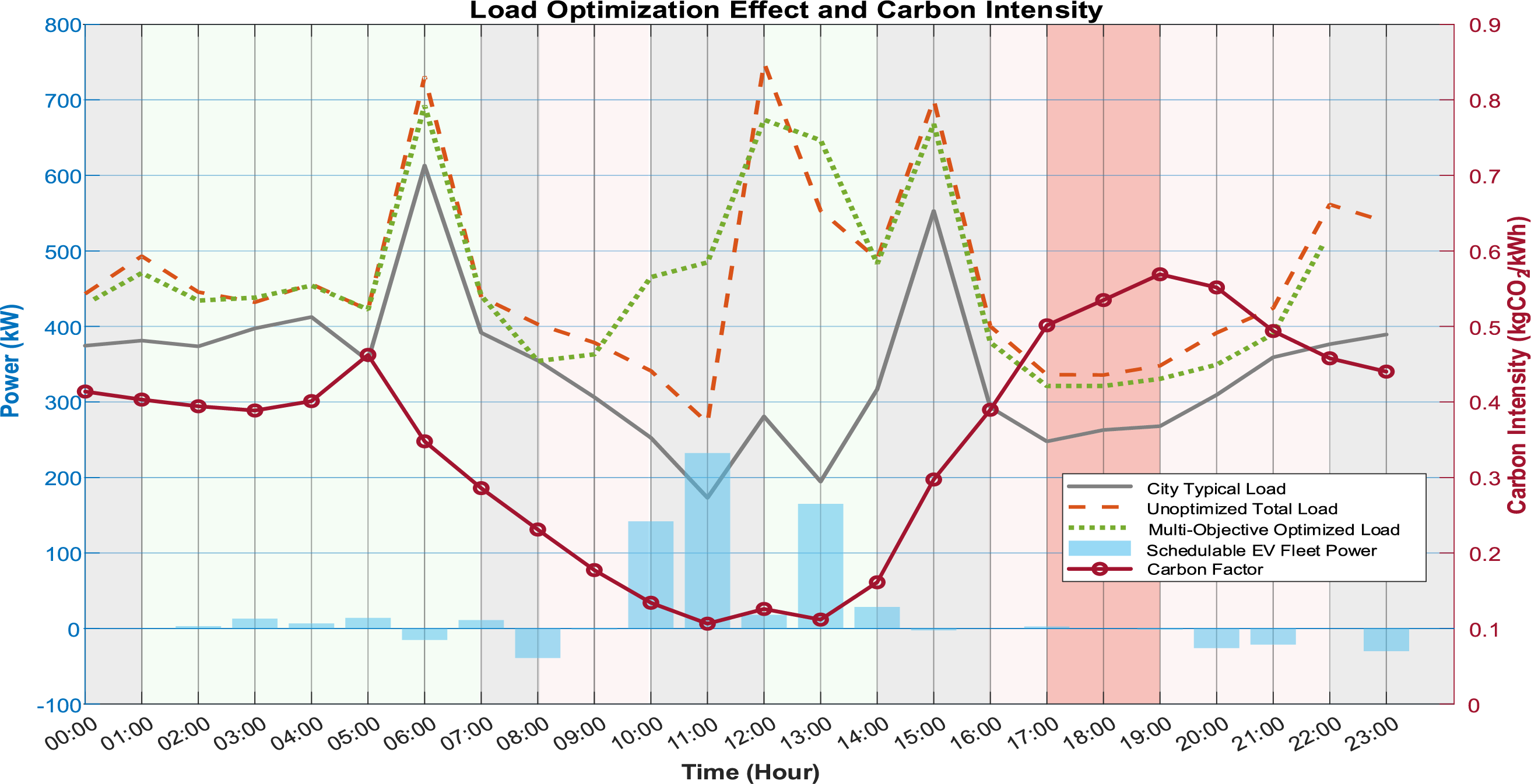
Figure 8: Load profile optimization and carbon intensity under the real-world data scenario
Fig. 8 visualizes the underlying strategies. The proposed multi-objective method (green dashed line) intelligently utilizes the schedulable EV fleet (light blue bars) for both valley-filling and arbitrage. Significant charging is concentrated in the midday load valley (11:00–14:00), which corresponds to the period of lowest carbon intensity. Furthermore, a clear V2G discharging event occurs around 07:00–08:00 to capitalize on high electricity prices, demonstrating the model’s sophisticated co-optimization capability.
Finally, at the individual vehicle level, the SOC trajectories in Fig. 9 confirm the model’s adherence to all operational constraints.

Figure 9: SOC trajectories of the heterogeneous EV fleet under multi-objective optimization
Fig. 9 shows that all 18 heterogeneous vehicles successfully charge from their various initial states to their required final states (≥75% SOC). The charging behavior is clearly coordinated, with a sharp, collective increase in SOC beginning around 11:00, aligning perfectly with the low-carbon and low-cost window. The discharging events are also visible for V2G-capable vehicles, validating that the aggregate behavior is a result of coordinated, physically plausible actions at the individual vehicle level.
Finally, to assess the robustness of our optimization strategy against the inherent uncertainties of forecasting, we conducted an additional sensitivity test. In this test, a ±10% random noise was artificially added to the carbon factor prediction sequence used as the input for the optimization. The results showed negligible degradation in the final objective outcomes, confirming that the proposed strategy exhibits strong inherent robustness to moderate forecast errors. The detailed methodology, data, and a comparative table for this test are provided in Appendix A.2, with quantitative results in Table A2.
4.3 Deployment Potential and Integration with Energy Management Systems
Beyond theoretical innovation, the proposed framework is designed with practical engineering viability at its core, contextualized within a major demonstration project by the State Grid Corporation of China. Its deployment strategy is specifically designed to address the spatio-temporal precision deficiencies of traditional carbon metering methods.
The core advantage this framework addresses is the granularity and latency shortcomings of grid-side carbon factor calculations. Grid-level calculations, which rely on computationally intensive power flow analysis, are often limited to an hourly resolution and are subject to communication delays. This temporal resolution is insufficient for the fine-grained guidance required for EV charging regulation. Our integrated “cloud-edge” deployment scheme is designed to overcome this specific challenge.
The framework’s two-module design ensures computational tractability. The Carbon Factor Prediction Module, based on the improved Crossformer, is first trained offline using historical nodal carbon factor data. Once trained, this lightweight model is deployed on an edge computing gateway at the charging station, which is specified with a 2.5 GHz 8-core CPU and 16 GB of RAM. To provide quantitative metrics, we benchmarked the prediction model’s performance on this hardware: the trained lightweight model has a file size of only 2.97 MB, an average inference latency of just 12.35 ms, and a total process memory footprint of approximately 428 MB during operation. These quantified results clearly demonstrate that our prediction model meets the requirements for real-time, efficient execution on the specified edge hardware. This “fine-and-fast on the edge” approach provides the real-time, high-granularity carbon signals that grid-level systems cannot.
These high-resolution forecasts can be used locally for accurate carbon metering. In parallel, the data can be uploaded to a cloud master station or load aggregator. Here, our framework proposes a flexible, hierarchical deployment strategy for the EV Optimization Scheduling Module. For medium-sized charging stations, the optimization model presented in this paper can be deployed directly on the edge gateway to manage local dispatch. For large-scale, regional fleet coordination (>100 vehicles), we recommend that the scheduling task be handled on a central cloud server, which can utilize a more mature framework like Model Predictive Control (MPC). In this scenario, our edge-deployed prediction model’s core value remains critical, as it provides the essential high-resolution carbon signal inputs to the cloud-based controller.
Consequently, the framework is positioned to act as an effective plug-in for existing Energy Management Systems (EMS). Load aggregators can integrate the predicted high-resolution carbon factor as a new dynamic constraint or weight into their current economic dispatch models. This synergistic architecture allows the proposed strategy to effectively enhance the spatio-temporal precision of both carbon metering and grid regulation without requiring a complete overhaul of existing infrastructure.
This paper introduces a novel framework that integrates a high-precision carbon factor forecasting model with a multi-objective EV dispatch optimization strategy. The primary innovations are twofold: Firstly, by enhancing the Crossformer model with a multi-scale feature enhancement module, the accuracy of dynamic carbon factor prediction is significantly improved. Secondly, by directly incorporating these dynamic forecasts, this work establishes a more precise carbon accounting paradigm that internalizes real-time carbon costs, enabling strategies that proactively avoid high-carbon periods.
Building upon these innovations, a four-objective optimization model was developed to synergistically manage grid stability, economic cost, and carbon emissions. The superiority of this model was validated through two comprehensive case studies. The initial simulation in Case Study One established the fundamental advantage of the multi-objective approach over single-objective strategies. This was further substantiated in a more rigorous second case study using real-world data from a renewable-heavy grid. In this complex scenario, the proposed multi-objective strategy demonstrated a superior balance, achieving significant reductions in both carbon emissions (15.8%) and economic costs (5.2%) while maintaining substantial grid stability improvements (22.2% peak-valley reduction). Its balanced performance significantly outperformed both the single-objective strategy and a state-of-the-art Model Predictive Control (MPC) benchmark, highlighting the advantage of a global optimization approach in finding the optimal trade-offs.
This study, by providing a high-precision forecasting tool and an effective multi-objective optimization strategy, facilitates a deeper understanding of dynamic carbon management. The proposed framework demonstrates significant potential for practical deployment within existing energy management systems, contributing to the future development of dynamic carbon accounting standards and the implementation of carbon-sensitive electricity pricing policies.
Acknowledgement: We are very grateful for the support and cooperation of North China Electric Power University.
Funding Statement: Supported by State Grid Corporation of China Science and Technology Project: Research on Key Technologies for Intelligent Carbon Metrology in Vehicle-to-Grid Interaction (Project Number: B3018524000Q).
Author Contributions: The authors confirm contribution to the paper as follows: Zixuan Meng: Methodology, Software, Validation, Formal Analysis, Investigation, Data Curation, Writing—Original Draft, Writing—Review & Editing, Visualization. Hongyu Wang: Conceptualization, Supervision, Project Administration, Funding Acquisition. Wenwu Cui: Conceptualization, Resources. Kai Cui: Conceptualization, Resources. Bin Li: Conceptualization, Formal Analysis. Wei Zhang: Investigation, Data Curation. Wenwen Li: Investigation, Data Curation. All authors reviewed the results and approved the final version of the manuscript.
Availability of Data and Materials: The data that support the findings of this study are available from the Corresponding Author, Zixuan Meng, upon reasonable request.
Ethics Approval: Not applicable.
Conflicts of Interest: The authors declare no conflicts of interest to report regarding the present study.
Nomenclature
| EV | Electric vehicle |
| ICB | Integrated Convolution Block |
| ASB | Adaptive Spectral Block |
| TSA | Two-Stage Attention |
| MSA | Multi-head Self-Attention |
| FFT | Fast Fourier Transform |
| IFFT | Inverse Fast Fourier Transform |
| V2G | Vehicle-to-Grid |
| SOC | State-of-Charge |
| R2 | Coefficient of determination |
| MAPE | Mean Absolute Percentage Error |
| MAE | Mean Absolute Error |
This appendix provides supplementary materials and detailed data that support the analyses presented in the main text.
This subsection provides the quantitative data to confirm that the State of Charge (SOC) for all V2G-capable electric vehicles remained strictly within the predefined operational limits of [10%, 90%].
A.2 Robustness Analysis to Forecast Errors
To quantify the performance of the proposed multi-objective optimization strategy in the face of forecast uncertainty, we conducted a sensitivity test. This test was designed to simulate a realistic scenario where the carbon factor predictions are subject to small, random errors.
The methodology was as follows: First, the optimal carbon factor sequence predicted by our model was taken as the “perfect forecast” baseline. Then, a “noisy forecast” sequence was generated by applying a multiplicative random noise within the range of [0.9, 1.1] to each point of the baseline sequence, simulating a ±10% random error. Second, the optimization scheduling was executed using this “noisy forecast” to produce a “test schedule”. Finally, the actual performance of this “test schedule” was evaluated by calculating all four key objectives—economic cost, carbon emissions, peak-valley difference, and load variance—using the original, noise-free “perfect forecast” as the ground truth.
The results are presented in Table A2.
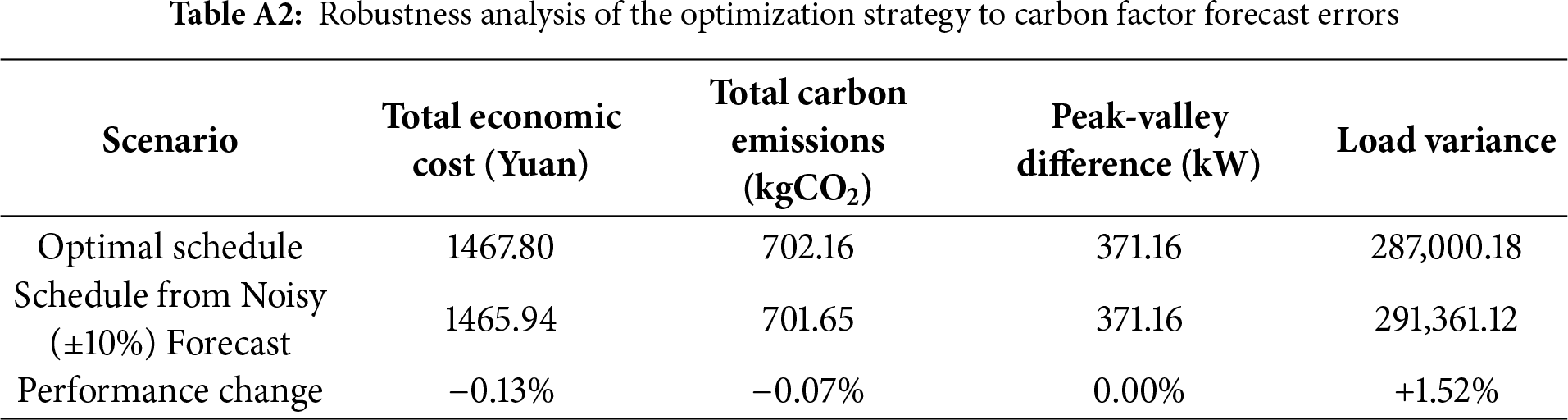
As shown in Table A2, even when the carbon factor predictions used for decision-making contain a ±10% random error, all key optimization objectives demonstrate a high degree of stability. Specifically, the changes in economic cost and carbon emissions are negligible. Crucially, the core grid-friendliness metric, the peak-valley difference, remains entirely unaffected, while the load variance shows only a minor increase. This comprehensive result clearly demonstrates that the proposed optimization framework possesses strong inherent robustness, effectively handling moderate uncertainties in its forecast inputs while maintaining stability across economic, environmental, and grid-friendliness objectives.
References
1. Lu Q, Fang H, Hou J. The impact of energy supply side on the diffusion of low-carbon transformation on energy demand side under low-carbon policies in China. Energy. 2024;307(4):132817. doi:10.1016/j.energy.2024.132817. [Google Scholar] [CrossRef]
2. Luo J, Zhuo W, Liu S, Xu B. The optimization of carbon emission prediction in low carbon energy economy under big data. IEEE Access. 2024;12(9):14690–702. doi:10.1109/ACCESS.2024.3351468. [Google Scholar] [CrossRef]
3. Miller GJ, Novan K, Jenn A. Hourly accounting of carbon emissions from electricity consumption. Environ Res Lett. 2022;17(4):044073. doi:10.1088/1748-9326/ac6147. [Google Scholar] [CrossRef]
4. Jin Y, Sharifi A, Li Z, Chen S, Zeng S, Zhao S. Carbon emission prediction models: a review. Sci Total Environ. 2024;927(14):172319. doi:10.1016/j.scitotenv.2024.172319. [Google Scholar] [PubMed] [CrossRef]
5. Chen X, Chao H, Shi W, Li N. Towards carbon-free electricity: a flow-based framework for power grid carbon accounting and decarbonization. arXiv:2308.03268. 2023. [Google Scholar]
6. Liu Z, Sun T, Yu Y, Ke P, Deng Z, Lu C, et al. Near-real-time carbon emission accounting technology toward carbon neutrality. Engineering. 2022;14(3):44–51. doi:10.1016/j.eng.2021.12.019. [Google Scholar] [CrossRef]
7. Kang C, Zhou T, Chen Q, Xu Q, Xia Q, Ji Z. Carbon emission flow in networks. Sci Rep. 2012;2(1):479. doi:10.1038/srep00479. [Google Scholar] [PubMed] [CrossRef]
8. Liu C, Guo Y, Qian X, Li X, Liu H, Zhong M. Understanding spatiotemporal dynamics of V2G participation in megacities: a data-driven study. Appl Energy. 2025;401:126866. doi:10.1016/j.apenergy.2025.126866. [Google Scholar] [CrossRef]
9. Fan H, Li M, Cui J, Zhang Z, Run W, Liu D. Spatiotemporal prediction of electric vehicle charging load based on large language models. arXiv:2506.03728. 2025. [Google Scholar]
10. Chen X, Sun A, Shi W, Li N. Carbon-aware optimal power flow. IEEE Trans Power Syst. 2025;40(4):3090–104. doi:10.1109/tpwrs.2024.3514516. [Google Scholar] [CrossRef]
11. Present E, Gagnon P, Wilson EJ, Merket N, White PR, Horowitz S. Choosing the best carbon factor for the job: exploring available carbon emissions factors and the impact of factor selection: preprint [Internet]. Washington, DC, USA: U.S. Department of Energy; 2024 [cited 2025 Oct 11]. Available from: https://www.osti.gov/biblio/2340119. [Google Scholar]
12. Peng TH, Cai X, Qu ZH, Tang AH, Shen R, Wang QM, et al. Research on calculation model of power supply carbon emission factor in regional power grid considering hierarchical and regional decoupling of large-scale power grid. Proc CSEE. 2024;44(3):894–905. (In Chinese). doi:10.13334/j.0258-8013.pcsee.222315. [Google Scholar] [CrossRef]
13. Shen X, Li J, Yin Y, Tang J, Lin W, Zhou M. Carbon emission factors prediction of power grid by using graph attention network. Energy Eng. 2024;121(7):1945–61. doi:10.32604/ee.2024.048388. [Google Scholar] [CrossRef]
14. Zhang B, Shao C, Han K. Carbon flow tracing method for power systems based on complex power distribution matrix. In: Proceedings of the 2023 IEEE 4th China International Youth Conference on Electrical Engineering (CIYCEE); 2023 Dec 8–10; Chengdu, China. Piscataway, NJ, USA: IEEE; 2024. p. 1–5. doi:10.1109/CIYCEE59789.2023.10401386. [Google Scholar] [CrossRef]
15. Zhou TR, Kang CQ, Xu QY, Chen QX. Preliminary investigation on a method for carbon emission flow calculation of power system. Autom Electr Power Syst. 2012;36(11):44–9. (In Chinese). [Google Scholar]
16. Zhou TR, Kang CQ, Xu QY, Chen QX. Preliminary theoretical investigation on power system carbon emission flow. Autom Electr Power Syst. 2012;36(7):38–43,85. (In Chinese). [Google Scholar]
17. Li B, Song Y, Hu Z. Carbon flow tracing method for assessment of demand side carbon emissions obligation. IEEE Trans Sustain Energy. 2013;4(4):1100–7. doi:10.1109/TSTE.2013.2268642. [Google Scholar] [CrossRef]
18. Liu YL, Li YW, Zhou CL, Song JW, Deng HY, Du ES, et al. Overview of carbon measurement and analysis methods in power systems. Proc CSEE. 2024;44(6):2220–36. (In Chinese). doi:10.13334/j.0258-8013.pcsee.223452. [Google Scholar] [CrossRef]
19. Li YW, Liu YL, Yang XB, He W, Fang YJ, Du ES, et al. Electricity carbon metering method considering electricity transaction information. Proc CSEE. 2024;44(2):439–51. (In Chinese). doi:10.13334/j.0258-8013.pcsee.222323. [Google Scholar] [CrossRef]
20. Li G, Wu H, Yang H. A multi-factor combination prediction model of carbon emissions based on improved CEEMDAN. Environ Sci Pollut Res Int. 2024;31(14):20898–924. doi:10.1007/s11356-024-32333-x. [Google Scholar] [PubMed] [CrossRef]
21. Shen X, Tang J, Li J, Zhao Y, Yin Y, Zhang F. TimesNet: an algorithm for day-ahead forecast of dynamic carbon emission factors in power grids. In: Proceedings of the 2024 6th Asia Energy and Electrical Engineering Symposium (AEEES); 2024 Mar 28–31; Chengdu, China. Piscataway, NJ, USA: IEEE; 2024. p. 1393–8. doi:10.1109/AEEES61147.2024.10544696. [Google Scholar] [CrossRef]
22. Zhou H, Zhang S, Peng J, Zhang S, Li J, Xiong H, et al. Informer: beyond efficient transformer for long sequence time-series forecasting. arXiv:2012.07436. 2020. [Google Scholar]
23. Liu Y, Wu H, Wang J, Long M. Non-stationary transformers: exploring the stationarity in time series forecasting. arXiv:2205.14415. 2022. [Google Scholar]
24. Liu Y, Hu T, Zhang H, Wu H, Wang S, Ma L, et al. iTransformer: inverted transformers are effective for time series forecasting. arXiv:2310.06625. 2023. [Google Scholar]
25. Zhang Y, Yan J. Crossformer: transformer utilizing cross-dimension dependency for multivariate time series forecasting. In: Proceedings of The Eleventh International Conference on Learning Representations; 2022 Apr 25–29; Virtual. [Google Scholar]
26. Sahoo JP, Sivasubramani S. A charging coordination strategy for seamless integration of plug-in electric vehicles into a distribution network. In: Proceedings of the 2023 IEEE IAS Global Conference on Renewable Energy and Hydrogen Technologies (GlobConHT); 2023 Mar 11–12; Male, Maldives. Piscataway, NJ, USA: IEEE; 2023. p. 1–6. doi:10.1109/GlobConHT56829.2023.10087580. [Google Scholar] [CrossRef]
27. Sahoo JP, Sivasubramani S, Srikar PSS. Optimized framework for strategic electric vehicle charging station placement and scheduling in distribution systems with renewable energy integration. Swarm Evol Comput. 2025;95(3):101943. doi:10.1016/j.swevo.2025.101943. [Google Scholar] [CrossRef]
28. Yan S, Li B, Zhang Y, Ye J, Yin W. A multi-objective optimization strategy for V2G-based scaled electric vehicles in distribution system with various PV penetration. In: Proceedings of the 2024 IEEE PES 16th Asia-Pacific Power and Energy Engineering Conference (APPEEC); 2024 Oct 25–27; Nanjing, China. Piscataway, NJ, USA: IEEE; 2025. p. 1–5. doi:10.1109/APPEEC61255.2024.10922597. [Google Scholar] [CrossRef]
29. Ahmadi SE, Kazemi-Razi SM, Marzband M, Ikpehai A, Abusorrah A. Multi-objective stochastic techno-economic-environmental optimization of distribution networks with G2V and V2G systems. Electr Power Syst Res. 2023;218(8):109195. doi:10.1016/j.epsr.2023.109195. [Google Scholar] [CrossRef]
30. Wu Z, Wang C, Dai X, Zhang X, Lu Z, Liang R. Long-term load forecasting method for electric vehicles aimed at regulation capability assessment. In: Proceedings of the 2024 6th International Academic Exchange Conference on Science and Technology Innovation (IAECST); 2024 Dec 6–8; Guangzhou, China. Piscataway, NJ, USA: IEEE; 2025. p. 1300–4. doi:10.1109/IAECST64597.2024.11117719. [Google Scholar] [CrossRef]
31. Vuelvas J, Ruiz F, Gruosso G. A time-of-use pricing strategy for managing electric vehicle clusters. Sustain Energy Grids Netw. 2021;25(4):100411. doi:10.1016/j.segan.2020.100411. [Google Scholar] [CrossRef]
32. Yang SY, Woo J, Lee W. Assessing optimized time-of-use pricing for electric vehicle charging in deep vehicle-grid integration system. Energy Econ. 2024;138(177):107852. doi:10.1016/j.eneco.2024.107852. [Google Scholar] [CrossRef]
33. Shahriar S, Al-Ali AR, Osman AH, Dhou S, Nijim M. Prediction of EV charging behavior using machine learning. IEEE Access. 2021;9:111576–86. doi:10.1109/ACCESS.2021.3103119. [Google Scholar] [CrossRef]
Cite This Article
 Copyright © 2026 The Author(s). Published by Tech Science Press.
This work is licensed under a Creative Commons Attribution 4.0 International License , which permits unrestricted use, distribution, and reproduction in any medium, provided the original work is properly cited.
 Downloads
 Citation Tools