Heterogeneous Graph Neural Network–Assisted Joint Clearing for Intra- and Inter-Provincial Electricity Spot Markets

1  Introduction

The national unified electricity market is a key component in the construction of a unified national market in China [1]. According to the central government’s unified plan, by the end of 2025, electricity spot markets are expected to achieve near-full coverage nationwide, with continuous settlement operations fully implemented, thereby enabling the spot market to play its crucial roles in price discovery and supply–demand regulation [2]. However, with the continuous growth of inter-provincial electricity transmission, the current approach—where each province independently organizes spot market transactions—can no longer meet the requirements of global resource optimization [3,4]. It is therefore imperative to advance market-oriented inter-provincial and inter-regional electricity trading, promoting the smooth flow of electricity resources on a national scale [5].

The inter-provincial electricity spot market enables power generators and consumers, on the basis of their participation in provincial spot markets, to leverage regional differences to achieve supply–demand balancing [6], ensure power supply, and facilitate the integration of renewable energy [7]. Regarding research on joint clearing between provincial and inter-provincial electricity spot markets, Ref. [8] proposed an inter-provincial electricity spot market model suitable for China, employing centralized optimization and marginal clearing to achieve coordinated day-ahead market clearing across regions. Ref. [9] introduced a path-aware inter-provincial market clearing model, where redundant elimination methods are adopted to effectively handle market clearing problems in hybrid AC/DC interconnected networks. Ref. [10] designed an optimal clearing model for both intra-provincial and inter-provincial transactions with network constraints, implementing coordinated optimization for multi-regional electricity markets via a joint clearing algorithm and a simplified grid model.

Research on cross-regional electricity market coupling and coordination mechanisms provides a theoretical basis for inter-provincial joint clearing. Ref. [11] analyzed key market mechanisms for cross-regional electricity trading from both theoretical and practical perspectives, focusing on the coordination between regional sub-markets and overarching regional markets. Ref. [12] evaluated cross-border integration issues in capacity mechanisms for coupled electricity markets, offering solutions for multi-market coordination. Ref. [13] investigated the impact of inter- and intra-regional coordination in power systems with large-scale renewable energy, verifying the effectiveness of market coupling mechanisms. Ref. [14] presented the integration of the European internal electricity market through market coupling, providing experience for large-scale market coordination. However, the above studies mainly focus on the mechanism design and theoretical framework construction of the inter-provincial market, but lack efficient solution strategies for the coupled clearing process of the intra-provincial and inter-provincial markets. Especially when facing the participation of a large number of market entities, traditional mathematical optimization methods are confronted with dual challenges of computational efficiency and scalability, leading to excessively long or even timed-out clearing calculation, which seriously restricts the real-time operation capability of the market.

With the continuous expansion and increasing complexity of power systems, traditional mathematical optimization methods face significant challenges in computational efficiency and scalability when solving large-scale inter-provincial joint clearing problems [15,16]. In recent years, with the rapid advancement of artificial intelligence technologies, graph neural networks (GNNs) have demonstrated promising applications in electricity market clearing optimization due to their capability to effectively process graph-structured data [17,18]. Ref. [19] applied neural network–constrained optimization methods to dynamically capture electricity market behavior, constructing surrogate models for market clearing by leveraging the nonlinear mapping capabilities of neural networks. Ref. [20] proposed a price-aware deep learning approach that embeds electricity market clearing optimization within a deep learning framework, effectively improving the uniformity of system price error distribution. Ref. [21] developed a machine learning–based market clearing method by building a machine-learning twin model for optimal power flow optimization, providing a new pathway to accelerate market clearing computations. However, existing auxiliary methods still have obvious limitations: on the one hand, most studies focus on the clearing problem at a single market level and fail to effectively depict the coupling relationship between intra-provincial clearing results and the screening of inter-provincial trading entities. On the other hand, current applications of Graph Neural Networks (GNNs) are mostly limited to electricity price prediction or static topology analysis, which are difficult to directly serve the efficient solution of large-scale Mixed Integer Linear Programming (MILP) joint clearing problems involving a large number of integer variables.

To address the aforementioned research gaps, this paper proposes a heterogeneous graph neural network (HGNN)-assisted joint clearing method for the intra-provincial and inter-provincial electricity spot markets. The main contributions of this study are as follows: first, a heterogeneous graph model covering generator units, loads, provincial nodes and tie-line nodes is constructed, and the complex correlation between the behaviors of intra-provincial market entities and the inter-provincial coordination mechanism is systematically depicted through the structural design of multi-type nodes and multi-relation edges; second, an HGNN-driven integer variable pre-identification strategy is proposed, which uses historical clearing data to train the model offline to generate high-quality initial solutions, significantly accelerating the convergence process. The results show that the proposed method effectively improves the computational efficiency of large-scale joint clearing problems while ensuring the optimality of clearing results.

2  Bi-Level Clearing Model for Intra- and Inter-Provincial Spot Markets

The intra- and inter-provincial electricity spot market clearing model proposed in this paper adopts a bi-level clearing mechanism. First, independent clearing is conducted within each province. Then, based on transmission line capacity constraints, a subset of market participants is selected to participate in the inter-provincial joint clearing. This approach significantly reduces the number of participants in inter-provincial trading, thereby improving computational efficiency. The procedure consists of the following five steps:

Step 1: Market Bid Submission.

Each market participant submits the energy bid and offer curves for all periods of the operating day according to the disclosure data released by the system operator.

Step 2: Independent Intra-Provincial Clearing.

Each province performs an independent market clearing to obtain the provincial clearing price and the awarded quantities of each participant for all time intervals.

Step 3: Participant Selection for Inter-Provincial Trading.

Based on the intra-provincial clearing results, each province selects participants that satisfy interconnection capacity limits and have the highest potential to be cleared in the inter-provincial market.

Step 4: Inter-Provincial Joint Clearing.

The selected market participants from all provinces jointly participate in the inter-provincial market clearing to obtain the final inter-provincial clearing results.

Step 5: Result Integration and Dispatch.

The inter-provincial clearing results are combined with the intra-provincial results and dispatched to the corresponding provincial market operators.

The overall process is illustrated in Fig. 1.

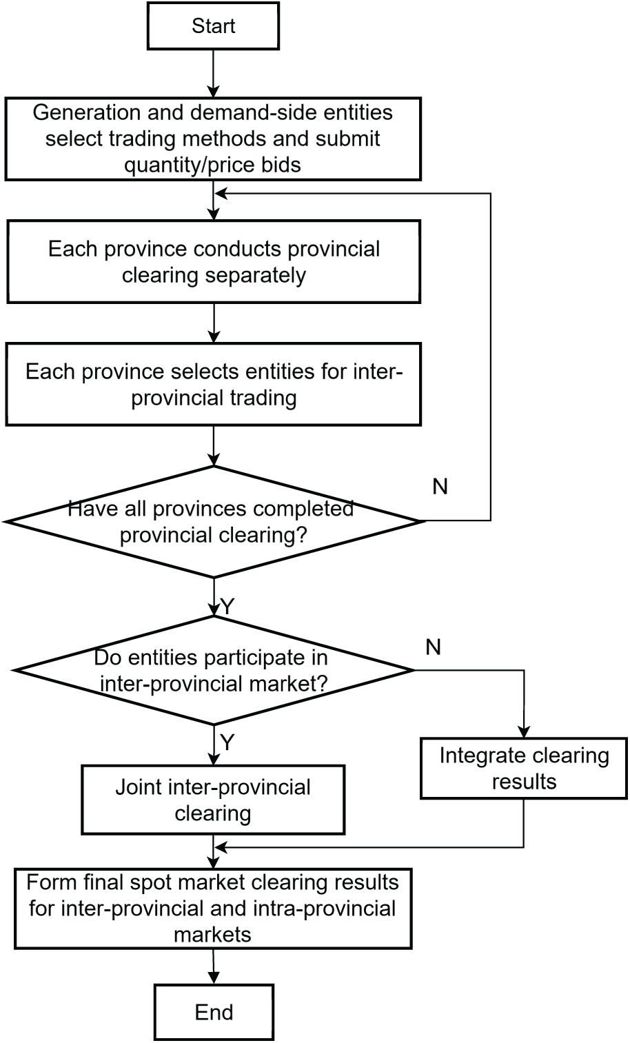
Figure 1: Flow chart of inter- and intra-provincial electricity spot market clearing

2.1 Independent Intra-Provincial Clearing Model

The independent intra-provincial clearing refers to the unified market clearing for all participants within each province. To simplify the problem, the proposed model performs hourly clearing, resulting in 24 clearing periods per day.

Let D denote the number of demand-side participants, G denote the number of generation-side participants, and N = D + G denote the total number of market participants in the intra-provincial electricity spot market.

The bid price of each market participant at time period t can be expressed as:

Sg,t={pg,t,qg,t}(1)

Sd,t={pd,t,qd,t}(2)

where Sg,t and Sd,t denote the bidding data of generation-side participant g and demand-side participant d at time period t; pg,t and pd,t denote the electricity price; qg,t and qd,t denote the electricity quantity.

2.1.1 Objective Function

The objective function of the intra-provincial electricity spot market clearing is to minimize the total operating cost of the provincial power grid, such that generation-side participants with lower bids and demand-side participants with higher bids are prioritized in the clearing process. The formulation is expressed as follows:

minxd,t,xg,t∑t[∑g=1G(xg,tpg,tqg,t)−∑d=1D(xd,tpd,tqd,t)](3)

where xd,t is the Boolean variable indicating the clearing status of demand-side participant d at time period t; xg,t is the Boolean variable indicating the clearing status of generation-side participant g at time period t.

2.1.2 Constraints

The clearing process of the intra-provincial electricity spot market is subject to multiple constraints, including intra-provincial power balance, operational constraints of both generation-side and demand-side participants, and unit commitment constraints. These are not elaborated here for brevity.

Instead of omitting constraints, the specific constraints involving integer variables are formulated as follows. These constraints introduce non-convexity, necessitating the HGNN-assisted approach.

(1)   Power Balance Constraint:

∑g=1Gqg,t−∑d=1Dqd,t=Lt,∀t(4)

(2)   Block Order Constraints: To accommodate diverse trading needs, block orders are considered. For a block order k spanning from time Tstart to Tend:

xk,t=xk,t+1,∀t∈[Tstart,Tend−1](5)

where xk,t represents the binary acceptance status.

(3)   Unit Operational Constraints: For generation units, the minimum up/down time constraints and ramping constraints are modeled as:

{∑τ=t−TUg+1tug,τ≤xg,t−RDg≤qg,t−qg,t−1≤RUg(6)

2.2 Participant Selection for Inter-Provincial Transactions

For entities selected to participate in inter-provincial transactions, the total submitted electricity quantity must not exceed the capacity of interconnection lines. Among the participants not awarded in the intra-provincial market, generation-side entities with lower bids and demand-side entities with higher bids are prioritized. Conversely, among those already awarded, generation-side entities with higher bids and demand-side entities with lower bids are given priority. Therefore, the selection of participants for inter-provincial trading can be formulated as an optimization problem.

2.2.1 Objective Function

The objective of the optimization is to prioritize, among the unawarded participants in the intra-provincial market, generation-side entities with lower bid prices and demand-side entities with higher bid prices; and among the awarded participants, generation-side entities with higher bid prices and demand-side entities with lower bid prices.

min∑t[∑g=1G(x¯g,tpg,tqg,t)−∑d=1D(x¯d,tpd,tqd,t)−∑g=1G(x_g,tpg,tqg,t)+∑d=1D(x_d,tpd,tqd,t)](7)

where x¯d,t and x¯g,t denote the participation status of unawarded demand-side and generation-side entities, respectively, in the inter-provincial market clearing. x_d,t and x_g,t denote the participation status of awarded demand-side and generation-side entities, respectively. All the above variables are Boolean, where a value of 0 indicates non-participation and a value of 1 indicates participation.

2.2.2 Constraints

The total declared electricity quantity by the entities selected to participate in inter-provincial transactions shall satisfy the capacity constraint of the inter-provincial tie lines.

∑d=1D(x¯d,tqd,t)=Pn_(8)

∑g=1G(x¯g,tqg,t)=Pn¯(9)

∑d=1D(x_d,tqd,t)=Pn¯(10)

∑g=1G(x_g,tqg,t)=Pn_(11)

where Pn¯ denotes the maximum amount of electricity that province n is allowed to export to other provinces. Pn_ denotes the maximum amount it is allowed to import. These values are determined based on the approved inter-provincial tie-line limits issued by the dispatching authority.

2.3 Inter-Provincial Market Clearing Model

The entities selected from each province in Section 2.2 participate in a unified inter-provincial market clearing process. The objective is to minimize the total operational cost of all provinces. Based on the assumption that transmission fees are excluded to focus on allocation efficiency, the transmission cost term is omitted. The formulation is updated as follows:

minXd,t,Xg,t∑t[∑g=1G(Xg,tpg,tqg,t)−∑d=1D(Xd,tpd,tqd,t)](12)

where Xg,t and Xd,t denote the final clearing results for generation-side entity g and demand-side entity d in time period t, respectively. Cj denotes the transmission price of tie line j. Tj,t denotes the transmission power on tie line j during time period t.

In addition to the intra-provincial clearing constraints, the inter-provincial market clearing model incorporates capacity constraints on the tie lines, ensuring that the transmission power on each tie line does not exceed its rated capacity. The transmission power of tie line j is calculated as:

Tj,t=Gj−g∑g=1G(Xg,tqg,t)−Gj−d∑d=1D(Xd,tqd,t)(13)

where Gj−g and Gj−d denote the sensitivities of generation-side entity g and demand-side entity d with respect to tie line j, respectively. The transmission power flow is calculated based on PTDFs (Power Transfer Distribution Factors), denoted as Gj−g for node n on line j. The tie-line constraint is formulated as:

−Pjmax≤∑nGj−n⋅Pinj,n,t≤Pjmax(14)

which establishes the physical coupling between provincial markets.

2.4 Key Model Assumptions

To define the boundary of the proposed joint clearing model and ensure the solvability of the problem, the following assumptions are made regarding market rules, participant behavior, and network constraints:

(1)   Centralized Clearing Mechanism: The intra- and inter-provincial markets operate under a centralized clearing mode. The market operator (ISO) collects all bids and offers and clears the market centrally to minimize the total system cost. Decentralized bilateral trading or continuous trading mechanisms are not considered in this formulation.

(2)   Rational Bidding Behavior: All market participants are assumed to be rational economic entities. They submit static bids representing their marginal costs or willingness to pay. Complex behavioral dynamics, such as strategic gaming, withholding capacity, or dynamic learning of bidding strategies during the clearing process, are not modeled. The focus is on the optimization of resource allocation given a set of submitted bids.

(3)   Transmission and Congestion Simplifications: While physical transmission limits (tie-line capacity) are strictly enforced as hard constraints (as defined in Eqs. (5)–(8) and Eq. (10)), the associated economic costs are simplified:

•   No Transmission Fees: Inter-provincial transmission tariffs (wheeling charges) are excluded from the objective function.

•   Physical Congestion Management: Congestion is managed by physically limiting power flow (re-dispatching generation) rather than by applying explicit congestion pricing in the cost function.

These assumptions allow the model to isolate and evaluate the computational efficiency of the HGNN-assisted approach in solving the core resource allocation problem.

3  Fast Solving Strategy Based on Heterogeneous Graph Neural Network

The intra-provincial clearing model, the participant selection model for inter-provincial trading, and the inter-provincial market clearing model described above all aim to minimize their respective objective functions under multiple constraints, while ensuring that certain decision variables are Boolean and take integer values. These problems can thus be formulated and solved as Mixed-Integer Linear Programming (MILP) models to obtain the final clearing results.

In practice, the total number of generation-side and demand-side entities involved in multi-provincial joint market clearing can reach tens or even hundreds of thousands. Consequently, the resulting MILP model contains a vast number of integer variables, making the problem NP-Hard. Conventional solvers often struggle with such large-scale problems, leading to long computation times and even timeout failures, which may disrupt market operations and settlement procedures.

To address this issue, this paper proposes a fast solving strategy assisted by heuristic rules, leveraging a heterogeneous graph neural network (HGNN) to pre-identify integer variables in the joint intra- and inter-provincial market clearing process, thereby improving computational efficiency. The proposed solution framework is illustrated in the figure. The proposed solution framework is shown in Fig. 2, and it consists of two main stages: offline training and online identification.

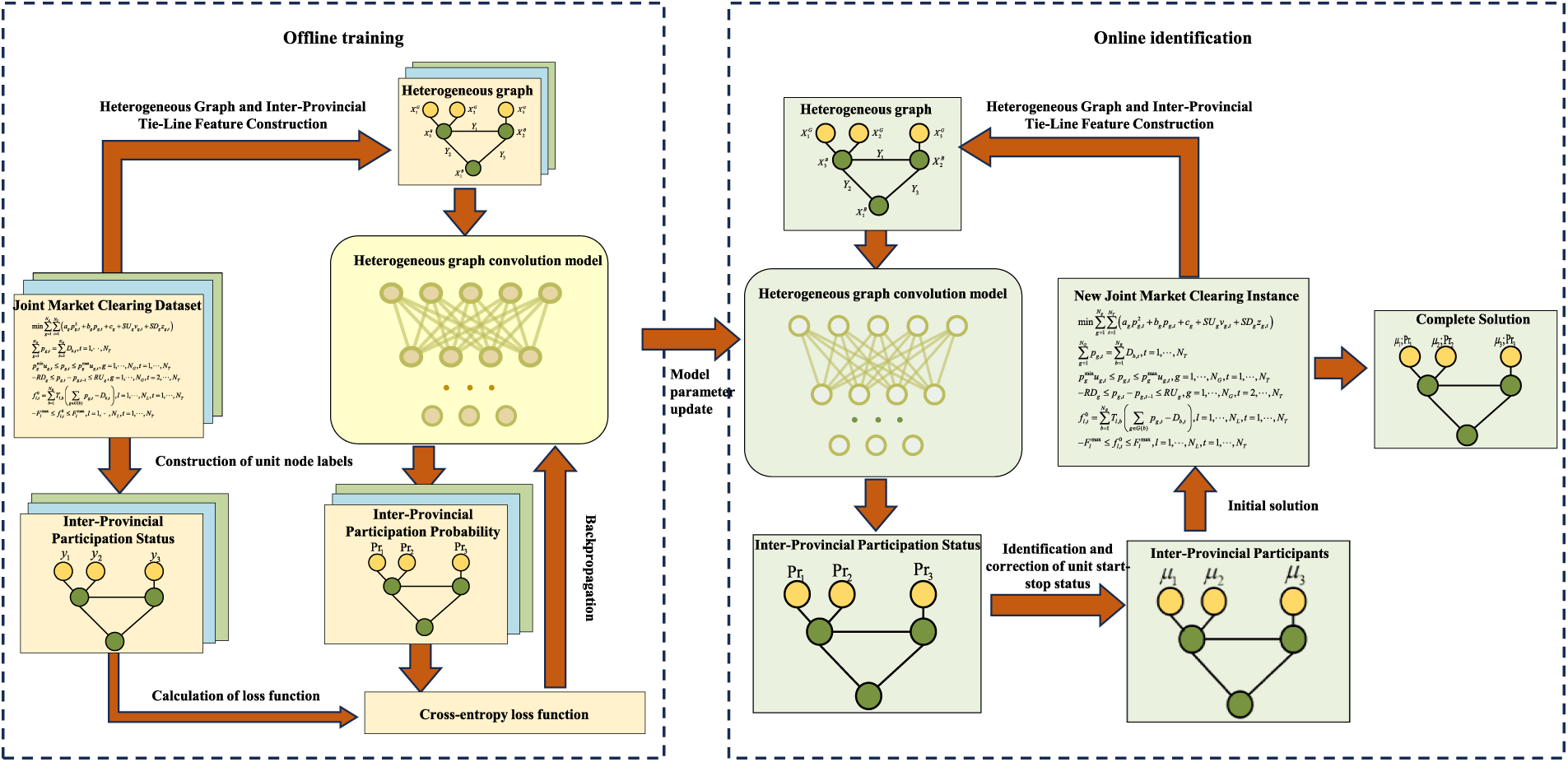
Figure 2: Heterogeneous graph neural network-assisted solving framework diagram

In the offline training phase, historical instances of joint intra- and inter-provincial market clearing are used to construct a dataset, incorporating the heterogeneous graph structure, tie-line features, and labels such as the clearing status (awarded or not) of generation-side and demand-side entities in both intra- and inter-provincial markets. A supervised learning approach is adopted to train the HGNN-based classification model. Once training is complete, the learned model parameters are transferred to the online inference model.

In the online inference phase, for a new clearing instance, the corresponding heterogeneous graph and node features are constructed and input into the HGNN model. The model outputs the predicted probabilities of each generation-side and demand-side entity being cleared in both intra- and inter-provincial markets. A correction mechanism is applied to the predicted results to ensure they satisfy the tie-line capacity constraints. The corrected identification results are then used as the initial solution for the solver, enabling it to rapidly converge to the optimal solution.

3.1 Construction of the Heterogeneous Graph

With respect to the provincial–inter-provincial electricity spot market bi-level clearing model presented in Section 1, the electricity market system is modeled in this study as a heterogeneous graph (HG). The purpose of constructing the HG is to capture, within a unified graph structure, the complex associations between the micro-level entities of provincial markets (such as generation units and loads) and the macro-level structures of the inter-provincial market (such as provinces and tie-lines), thereby providing the data basis for addressing the MILP problem in the bi-level optimization model. The node set of the HG comprises multiple types of entities, where generation-unit nodes represent the generation units within each province and are characterized by attributes such as unit type, generation capacity, and bid curves; load nodes represent the electricity demand within each province and include attributes such as load level and bid curves; province nodes serve as an abstract representation of the provincial market and encompass attributes including provincial power-balance status and tie-line capacities; and tie-line nodes represent the interconnections linking different provinces and are described by attributes such as transmission capacity and transmission losses. In addition, the edge set encodes multiple relationships among nodes, primarily including generation-unit–province and load–province edges that connect generation and load nodes to their corresponding provincial nodes, as well as province–tie-line edges that connect adjacent provincial nodes to the relevant tie-line nodes. This modeling approach provides a unified representation of market participants, provincial markets, and the inter-provincial market described in Section 1, thereby laying the groundwork for subsequent processing by the graph neural network. The power system is modeled as a graph 𝒢=(𝒱,ℰ). The node set 𝒱 consists of subset 𝒱G (Generators), 𝒱D (Loads), 𝒱P (Provinces), and 𝒱L (Tie-lines). The edge set ℰ represents the physical and market connections. Specifically, for a relation type r, the adjacency matrix is denoted as Ar. The feature matrix for node type ϕ is denoted as Xϕ. For example, the generator node feature xg∈XG includes {Pgmax,Pgmin,Rup,Rdown,Ton,Toff}.

3.2 Heterogeneous Graph Neural Network Model

The proposed heterogeneous graph neural network (HGNN) is designed to exploit both the structural information of the HG and the associated node features to rapidly pre-identify the mixed-integer variables in the bi-level model of Section 1, thereby generating a high-quality initial solution that accelerates the solution process. The model includes several core modules.

3.2.1 Heterogeneous Graph Embedding and Convolution Layer

This layer embeds the features of different node types in the HG by mapping the original feature vectors into a unified low-dimensional space. Because the feature dimensions and attribute characteristics differ across node types, type-specific linear projection matrices are employed to transform the features of each node type.

For generation-unit nodes vg, load nodes vd, province nodes vp, and tie-line nodes vl, their feature embeddings can be expressed as:

hg=Wgxg(15)

hd=Wdxd(16)

hp=Wpxp(17)

hl=Wlxl(18)

where xg, xd, xp and xl denote the original feature vectors of generation-unit, load, province, and tie-line nodes, respectively, and Wg, Wd, Wp and Wl represent the corresponding learnable weight matrices.

For a node i and relation type r, the feature aggregation is formulated as:

hi(l+1)=σ(∑r∈ℛ∑j∈𝒩ir1ci,rWr(l)hj(l)+W0(l)hi(l))(19)

where hi(l) is the hidden state of node i at layer l, 𝒩ir is the set of neighbors under relation r, and Wr(l) is the learnable weight matrix specific to relation r.

3.2.2 Edge-Feature Attention (EGAT) for Tie-Lines

Since inter-provincial tie-lines have crucial features (capacity limits), we employ an attention mechanism:

eij=LeakyReLU(aT[Whi||Whj||Wexij])(20)

αij=softmax(eij)(21)

This allows the model to weigh the importance of neighbor nodes dynamically based on tie-line congestion status.

3.2.3 Heterogeneous Graph Aggregation Layer

The aggregation layer constitutes the core of the HGNN, serving to integrate the information from neighboring nodes in order to update the representation of a central node. Given that the heterogeneous graph contains multiple types of edges, a meta-path-based aggregation mechanism is adopted in this study to differentiate the influence of various relationship types on node representations. A meta-path is defined as a sequence of node types; for example, the meta-path “generation unit–province–tie-line” can represent the association of a generation unit with an inter-provincial tie-line through its corresponding province. Such a meta-path-based aggregation strategy enables the targeted capture of semantic information associated with different relationship types. Furthermore, to evaluate the relative importance of neighboring nodes during the aggregation process, an attention mechanism is introduced. The attention network computes, for each neighbor node u and central node v, an attention coefficient αvu, which reflects the extent to which the neighbor node contributes to the update of the central node’s representation. The derivation of the attention coefficient is as follows:

First, the attention score is obtained through a learnable attention vector α and a nonlinear activation function, indicating the importance of node u to node v under a given meta-path r:

evur=LeakyReLU(aT[Wrhu‖Wrhv])(22)

where hu and hv denote the vector representations of the neighbor node u and the central node v after passing through the embedding layer, respectively; Wr is the type-specific transformation matrix associated with the meta-path r; ‖ denotes the vector concatenation operation.

Subsequently, the attention scores are normalized via the Softmax function to obtain the final attention coefficients αvur:

αvur=exp⁡(evur)∑k∈Nvrexp⁡(evkr)(23)

Through the attention mechanism, the model can adaptively focus on the neighboring information that is most relevant to the current task, namely the pre-identification of integer variables, thereby generating more discriminative node representations. The final aggregation process can be expressed as follows:

hv′=σ(∑r∈R∑u∈Nvrαvur(Wrhu))(24)

where R denotes the set of all meta-paths, Nvr denotes the set of neighbors connected to node v via meta-path r; αvur denotes the attention coefficients that quantify the importance of each neighbor node u to the central node v.

3.2.4 Heterogeneous Graph Aggregation Layer

After multiple layers of heterogeneous graph aggregation, the HGNN generates node embedding vectors that encapsulate rich structural information. The output layer utilizes these embeddings to perform classification or regression tasks for the pre-identification of the mixed-integer variables in the bi-level model presented in Section 1. In this study, the output layer of the HGNN is designed as a multi-layer perceptron (MLP), which takes the final node embeddings as input and outputs a probability value between 0 and 1, representing the likelihood that a given variable takes the value 1.

3.3 Output & Loss

The final node embeddings are passed through an MLP to predict the probability y^g,t of a generator being committed (or a block order being accepted). The model is trained using the Binary Cross-Entropy (BCE) loss function:

L=−1N∑i=1N[yilog⁡(y^i)+(1−yi)log⁡(1−y^i)](25)

where yi is the ground-truth binary value obtained from historical optimal solutions.

3.4 Feasibility Correction and MILP Integration Strategy

The raw probability outputs from the HGNN may inherently violate temporal constraints, such as the minimum up/down time of generation units, leading to infeasible initial solutions for the MILP solver. To address this, we propose an integration mechanism consisting of Interval-based Consistency Correction and Confidence-based Variable Fixing.

3.4.1 Interval-based Consistency Correction

To ensure the identified integer variables satisfy minimum up/down time constraints (Tgon,Tgoff), we calculate the Interval Average Confidence (μ) for any potential state change.

For a generator g at time t, the interval startup confidence μg,tU is defined as:

μg,tU=1Tgon∑τ=tt+Tgon−1Prg,τ(26)

where Prg,τ is the HGNN predicted probability of being “ON”. A heuristic correction rule is applied, if the unit status changes from 0 to 1 at time t, and μg,tU>δ, the startup is confirmed, and variables in the window [t,t+Tgon−1] are fixed to 1. Otherwise, the startup is deemed a false positive, and the status is corrected to 0. Moreover, a similar logic applies to shutdown processes using minimum down time Tgoff.

3.4.2 Integration with MILP Solver

The corrected binary variables are integrated into the MILP model using a Partial Fixing Strategy to prevent suboptimal search paths. First, variables with corrected probabilities near 0 or 1 are fixed as parameters in the CPLEX/Gurobi solver. This drastically reduces the combinational search space (Branch-and-Bound nodes). Second, variables with intermediate probabilities (indicating uncertainty) are left as free binary decision variables. The solver then optimizes these specific variables to find the global optimum, ensuring that HGNN prediction errors do not lock the system into a suboptimal state.

3.5 Solution Procedure

The overall procedure of the HGNN-assisted solution strategy is as follows:

Step 1: Data Preprocessing and Graph Construction. Based on the market bid data, grid topology information, and other relevant data from the bi-level model in Section 1, a heterogeneous graph is constructed comprising multiple types of nodes, including generation units, loads, provinces, and tie-lines, and the initial node features are extracted.

Step 2: HGNN Training. Historical clearing results are used as labels to train the HGNN model, enabling it to learn the optimal patterns of integer variable values from the graph structure and node features.

Step 3: Prediction and Initial Solution Generation. For new clearing tasks, the constructed heterogeneous graph is input into the trained HGNN model to predict the probability values of the mixed-integer variables.

Step 4: Feasibility Correction and Variable Fixing. The raw predictions are processed through the Interval-based Consistency Check. Based on the corrected results, a subset of integer variables is fixed. Specifically, variables satisfying the consistency check with high confidence are treated as constants, while low-confidence variables remain as integers to be solved.

Step 5: Reduced-Space MILP Solving. The simplified MILP model, with a significantly reduced number of free integer variables, is solved using a commercial solver. Since the fixed variables are pre-validated for temporal feasibility, the solver avoids exploring infeasible branches, and the retention of free variables prevents the exclusion of the global optimal solution.

4  Case Studies

To verify the applicability and superiority of the proposed joint intra- and inter-provincial electricity spot market clearing method in multi-regional power systems, three representative regions are constructed as study cases. The test system is designed based on a typical regional division logic, simulating the heterogeneity among provinces in terms of generation–consumption structure and load levels. A comparative analysis is conducted between the independent intra-provincial clearing and the joint intra- and inter-provincial clearing mechanisms.

4.1 Experimental Comparative Analysis

The experimental setup is based on a modified IEEE RTS-96 system, partitioned into three provinces to simulate the multi-regional market defined in Section 2. The generation-side entities (G in Eq. (3)) correspond to the 96 generating units in the RTS-96 system.

To comprehensively evaluate the performance and scalability of the proposed model in a multi-regional market environment, this study adopts a modified benchmark system based on the IEEE Reliability Test System 1996 (IEEE RTS-96) Three-Area System [Fig. 3]. The numerical scale and key definitions of the benchmark case are detailed as follows: System Topology (Provinces): The system comprises 3 provinces (corresponding to Areas A, B, and C of the RTS-96). As illustrated in the improved IEEE-96 interconnection line architecture diagram (Fig. 3), the three provinces form a ring-structured trading topology. Specifically, Province 1 and Province 2 are interconnected via three 230 kV tie-lines (L113-215, L123-217, and L107-203), while Province 3 is connected to Province 1 (L121-325) and Province 2 (L223-318) via single tie-lines, respectively. Nodes: The system consists of 73 buses in total. Province 1 and Province 2 each contain 24 nodes, while Province 3 includes 25 nodes (incorporating the interconnection node #325). Bidders: All generation and demand entities at topological nodes are active market participants. The benchmark includes 147 bidders, comprising 96 generation units (32 per province, covering thermal, nuclear, and hydro types) and 51 load aggregators (17 load nodes per province). Lines: The network contains 120 transmission branches, including 115 intra-provincial lines and the 5 critical inter-provincial tie-lines shown in Fig. 3. Strict Available Transfer Capability (ATC) limits are imposed on these tie-lines to simulate inter-provincial congestion scenarios. Detailed system parameters are summarized in Table 1.

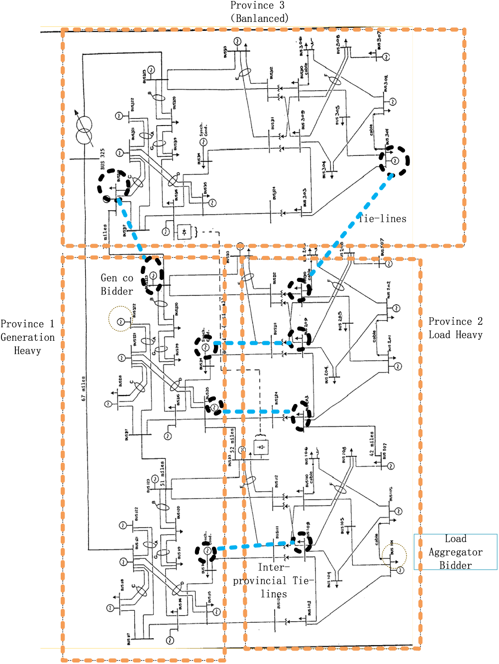
Figure 3: Intro-provincial structure based on modified IEEE-96 node

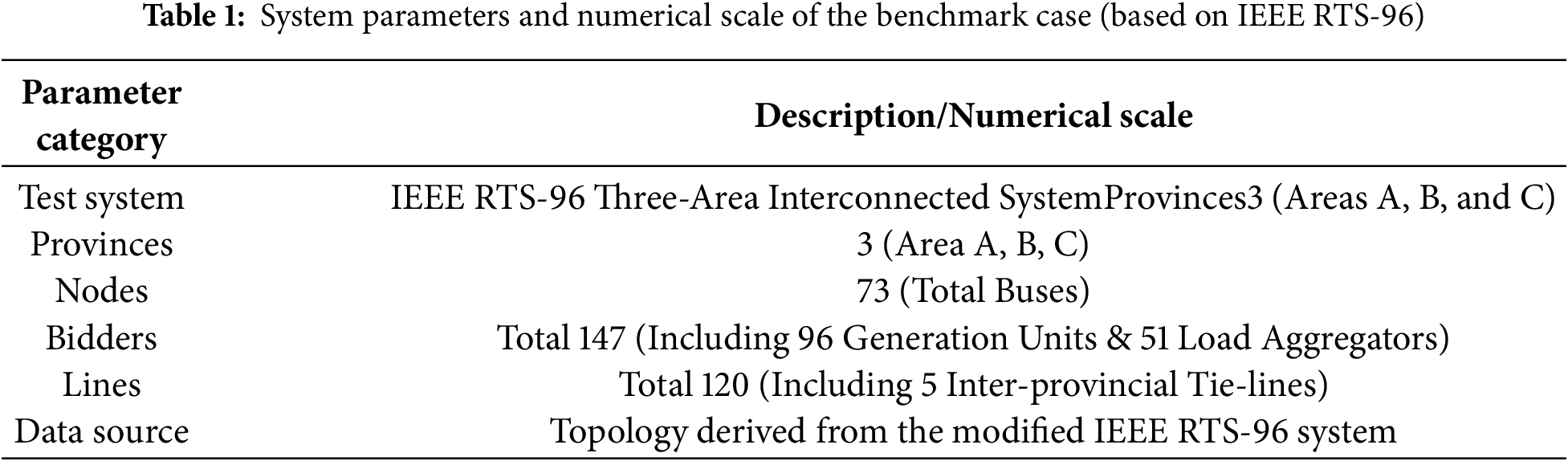
Fig. 4 presents the intra-provincial and inter-provincial clearing prices of the three regions, while Fig. 5 compares the trading volumes under the independent intra-provincial clearing and joint intra- and inter-provincial clearing mechanisms.

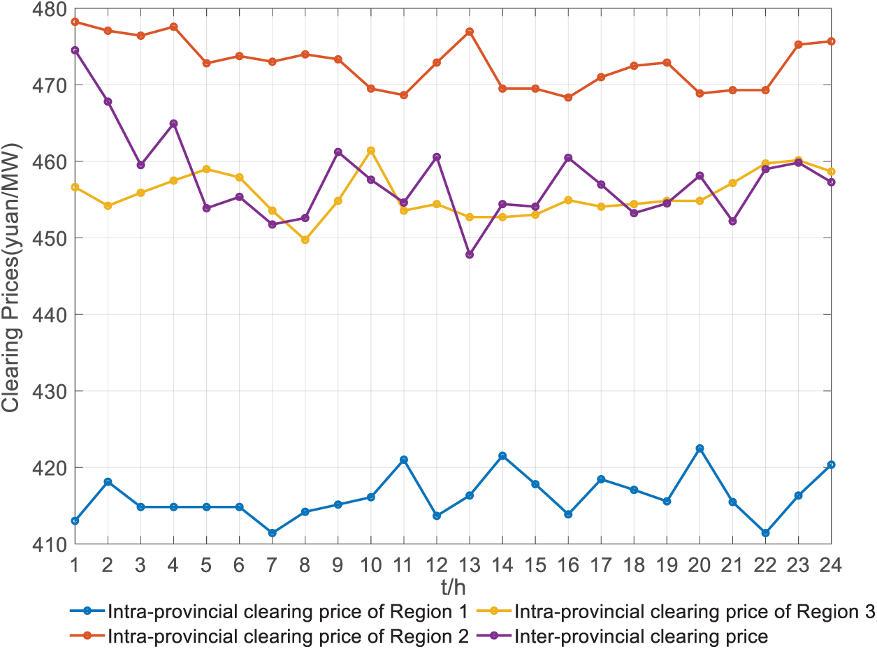
Figure 4: Clearing prices

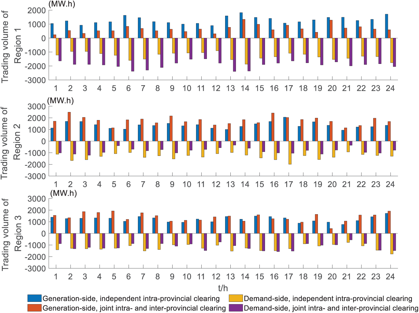
Figure 5: Clearing results of the three regions

Under the provincial–inter-provincial joint clearing mechanism, each region exhibits significant differences in both the traded electricity volumes on the generation and demand sides as well as in the clearing prices, reflecting the impact of cross-provincial resource coordination on market operations. In Region 1, the generation-side cleared volume under the joint clearing mode is generally lower than that under the provincial independent clearing mode, indicating that a portion of local generation load is substituted by low-cost external power, thereby achieving an optimized allocation of generation resources across provinces. This phenomenon is highly consistent with the price signals: the intra-provincial clearing price in Region 1 remains at the lowest level, and under joint clearing, it assumes a low-price export function, providing power support to high-price regions. At the same time, the absolute traded volume on the demand side increases compared with independent clearing, suggesting that cross-provincial electricity purchases effectively compensate for local demand, particularly mitigating potential supply–demand conflicts during morning and evening peak periods. Observing the daily curve, Region 1 exhibits an export-oriented operation driven by low-price advantage, while the demand side obtains stable supply through cross-provincial transactions, and the fluctuations in traded volumes are significantly reduced.

The overall trends in Regions 2 and 3 are similar. Taking the results from Region 2 as an example for analysis, in contrast to Region 1, the generation-side cleared volume in Region 2 under the joint clearing mode is generally higher than that under independent clearing, with the most pronounced differences occurring during morning and evening peak periods. This indicates that the introduction of inter-provincial resources optimizes power distribution and enhances the local units’ ability to absorb electricity. This trend is consistent with the price variations: the intra-provincial clearing price in Region 2 remains at a high level, attracting power inflows from low-price regions under price-driven incentives, thereby alleviating supply–demand tightness during peak periods. Meanwhile, the absolute traded volume on the demand side decreases under joint clearing compared with independent clearing, reflecting that part of the load is directly satisfied by cross-provincial electricity, reducing dependence on the local market. The daily trading curves indicate that under the joint clearing mode, fluctuations in electricity volumes are significantly smoothed, while inter-provincial clearing prices dynamically adjust between low- and high-price provinces, making the overall system operation more stable and efficient.

Based on the overall estimation from the Table 2, the calculation of 1201.2 + 436.8 − 1310.4 = 327.6 (104 CNY) indicates that the total cost under the independent provincial clearing mechanism is higher, whereas the total cost under the joint clearing mechanism (inter-provincial plus intra-provincial) is lower. Region 1 exhibits a lower intra-provincial clearing price. From a supply-demand perspective, this implies that the region is rich in generation resources. By participating in the inter-provincial market, it can sell electricity to other provinces to obtain higher revenue, thus functioning as a power-exporting province. Conversely, Region 2 has a higher intra-provincial clearing price. Supply-demand analysis suggests a scarcity of generation resources in this region. Upon joining the inter-provincial market, it can procure lower-priced electricity from other provinces, identifying it as a power-importing province. In Region 3, the intra-provincial clearing price aligns with the joint clearing price, implying that the region’s internal supply-demand balance is synchronized with the overall grid level, with no significant resource surplus or shortage.

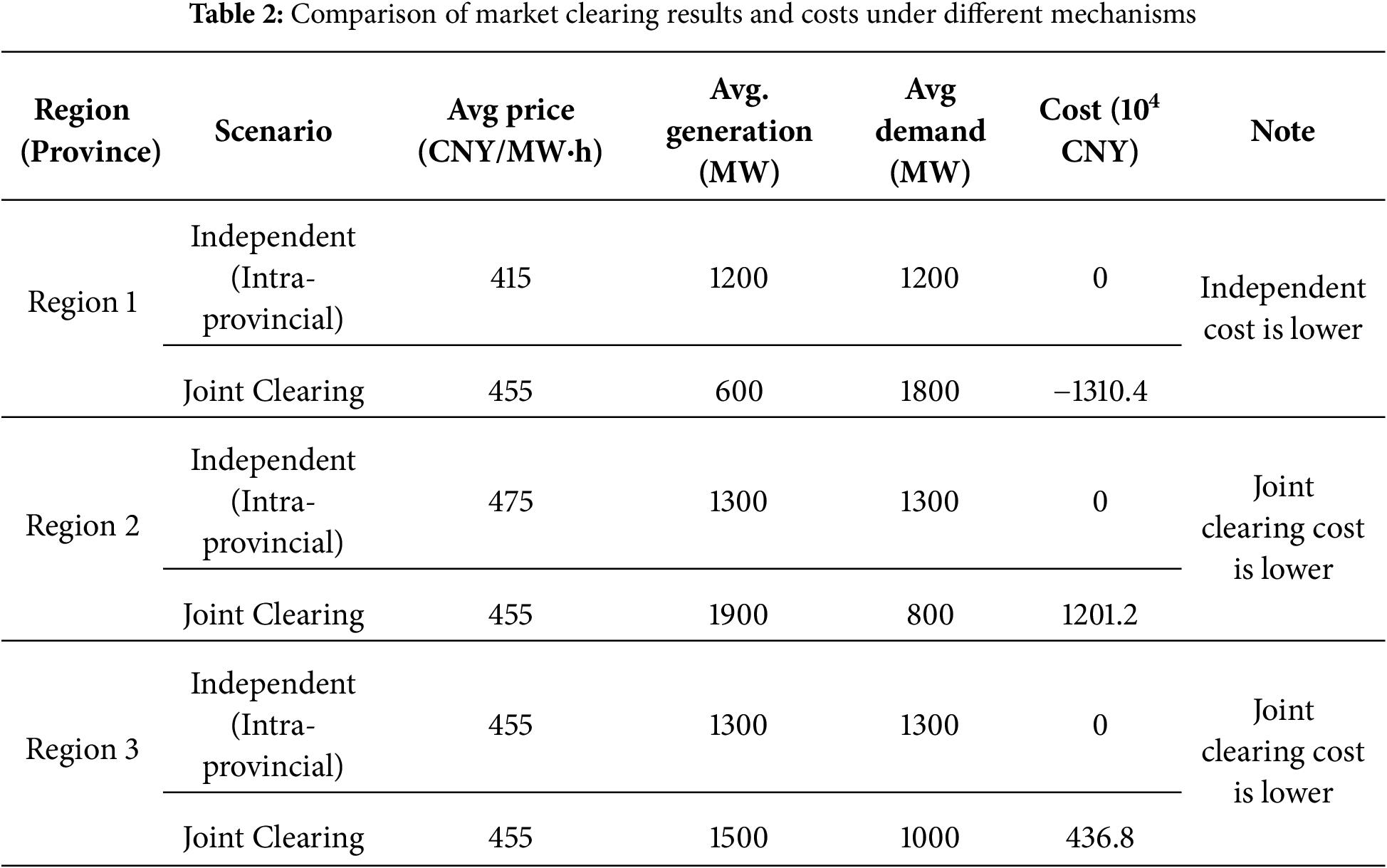
In summary, the provincial–inter-provincial joint clearing mechanism, guided by price signals, fully exploits the complementary potential between regions: low-price areas assume an export role, high-price areas receive power support, and the demand side achieves stable local supply through cross-provincial transactions. This mechanism not only promotes optimized allocation of electricity resources over a larger geographical scale but also significantly enhances the economic efficiency, flexibility, and coordinated operation of multi-regional electricity markets.

4.2 Sensitivity Analysis on Inter-Provincial Congestion

4.2.1 Evaluation Metrics

To comprehensively evaluate the economic efficiency and computational performance of the proposed HGNN-assisted joint clearing method, the following three metrics are selected:

(1)   Average Total Cost (Avg. Cost):

This metric represents the objective function value (social welfare or total operation cost) obtained by the clearing model. It serves as a direct indicator of the economic quality of the solution. The unit is million CNY (106 CNY). It is calculated as:

Avg.Cost=1Ntest∑i=1NtestZi(27)

where Ntest is the number of test instances, and Zi is the objective function value of the i-th instance.

(2)   Optimality Gap (Gap):

This metric quantifies the proximity of the solution obtained by the proposed method to the global optimal solution found by the traditional MILP solver (without variable fixing). It is defined as:

Gap=|ZHGNN−ZMILP|ZMILP×100%(28)

where ZHGNN is the cost obtained by the HGNN-assisted method, and ZMILP is the benchmark optimal cost. A lower gap indicates a higher solution quality.

(3)   Average Iterations (Avg. Iter.):

This metric measures the computational complexity of the solving process. It refers to the average number of Branch-and-Bound nodes or Simplex iterations performed by the solver to reach convergence. A significant reduction in iterations demonstrates the effectiveness of the HGNN in pruning the search space.

4.2.2 Scenarios Setup

If there is channel congestion between provinces (80% of the original channel capacity), there will be a new transaction volume and welfare result, dropping to approximately 70% of the unblocked scenario. Due to the increase in congestion costs, total social welfare decreases, and inter-provincial transaction volume also decreases. As congestion increases, more provinces tend to conduct intra-provincial trading rather than inter-provincial trading. The three scenarios are shown in the Table 3:

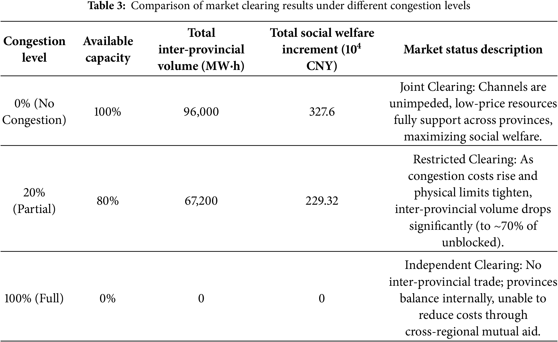
For Generation-Type Provinces (Region 1): In the absence of congestion, Region 1 utilizes its low electricity price advantage to export in large quantities, with its generation-side winning volume far exceeding local demand. However, as congestion occurs (from 0% to 20% and then to 100%), its “outward transmission channel” becomes blocked, and local low-price units are forced to reduce output, targeting only the satisfaction of intra-provincial load.

For Receiving-Type Provinces (Region 2): In the absence of congestion, Region 2 depresses excessively high intra-provincial marginal prices by importing cheap electricity. When channel congestion intensifies and external power input is restricted, Region 2 must call upon high-cost intra-provincial units, leading to an increase in overall power purchase costs and a loss of social welfare.

Clearing methods that consider inter-provincial transmission fees result in reductions in both total social welfare and total transaction volume. Although essentially beneficial for the economic efficiency of the overall clearing and reducing line losses, it simultaneously reduces inter-provincial transaction volume.

4.3 Algorithm Performance Analysis

To evaluate the computational efficiency of the proposed joint intra- and inter-provincial clearing method, the feasible solution rate, number of branch-and-bound nodes, and solving time of traditional solver-based methods and four model types—DNN, CNN, LSTM, and HGNN—were comparatively analyzed. The results are presented in Table 4, and the solving times of the four algorithms are illustrated in Fig. 5.

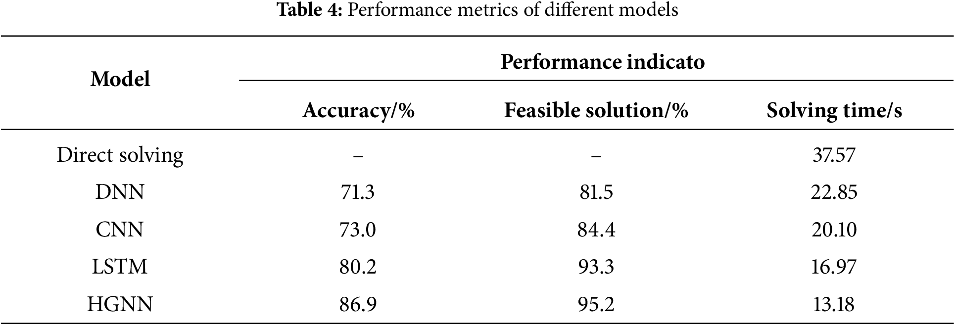
As shown in Table 4, different models exhibit significant differences in clearing accuracy, feasible solution rate, and solving time. The traditional direct solving method, without incorporating any learning assistance, relies solely on the solver’s inherent branch-and-bound mechanism to complete the optimization process. Its computation time is 37.57 s, indicating relatively low solving efficiency and insufficient timeliness for large-scale real-time market clearing applications.

In contrast, the DNN, CNN, and LSTM models substantially reduce computation time compared with direct solving. However, due to their limited ability to exploit structural correlations among nodes, their recognition accuracy and feasible solution rates remain suboptimal. The solving times of these three models are 22.85, 20.10, and 16.97 s, respectively, with feasible solution rates of 81.5%, 84.4%, and 93.3%. These results demonstrate their advantage in rapidly generating feasible solutions. Nevertheless, as these models primarily adopt planar feature-mapping structures, they fail to adequately capture the topological dependencies between intra-provincial and inter-provincial nodes, leading to deficiencies in accuracy.

The HGNN model further enhances overall performance, achieving an accuracy of 86.9%, a feasible solution rate of 95.2%, and a reduced solving time of 13.18 s. This result indicates that HGNN can effectively capture the coupling relationships between intra-provincial and inter-provincial nodes. By leveraging the graph-structured information propagation mechanism, it enables efficient identification of integer decision variables, thereby providing high-quality initial solutions for the optimizer and resulting in a more stable and efficient solving process.

As can be seen from Fig. 6, as the batch size increases, the computation time of all models shows a decreasing trend, indicating that model inference efficiency is improved under the combined effect of iterative training and batch processing optimization.

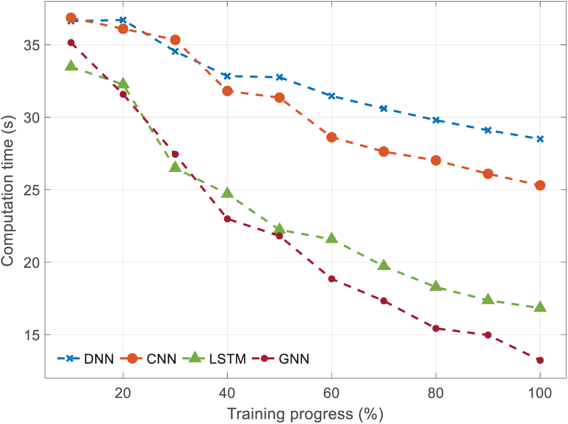
Figure 6: Comparison of algorithm computation times

From the model performance comparison, the HGNN consistently achieves the best performance, with the largest reduction in computation time. This demonstrates the significant advantages of graph-structured modeling in capturing multi-regional power system topological correlations, reducing redundant computations, and improving clearing efficiency. LSTM ranks second, benefiting from effective temporal feature extraction in dynamic clearing tasks, but its performance is slightly inferior to HGNN due to the lack of explicit utilization of spatial structural information. CNN and DNN exhibit longer computation times with relatively flat declining trends, indicating that relying solely on convolutional or fully connected architectures is insufficient to efficiently characterize the complex spatiotemporal dependencies of the joint clearing problem.

Table 5 presents a comparative analysis of the average total clearing cost, optimality gap, and convergence iterations for each algorithm, while Fig. 7 visualizes their iterative convergence behaviors regarding the objective function. As shown by the red line in Fig. 6, the proposed HGNN demonstrates the fastest convergence speed. While the Direct Solving approach attains the theoretical global optimum (12.45 × 106 CNY), it comes at the cost of extensive iterations (2450). Conversely, the HGNN method achieves a comparable total cost of 12.46 × 106 CNY with a negligible optimality gap of 0.08%, significantly superior to the gaps observed in LSTM (1.60%), CNN (4.25%), and DNN (5.38%). Moreover, with convergence achieved in just 320 iterations, the HGNN reduces the computational burden by approximately 87% compared to the direct solving method.

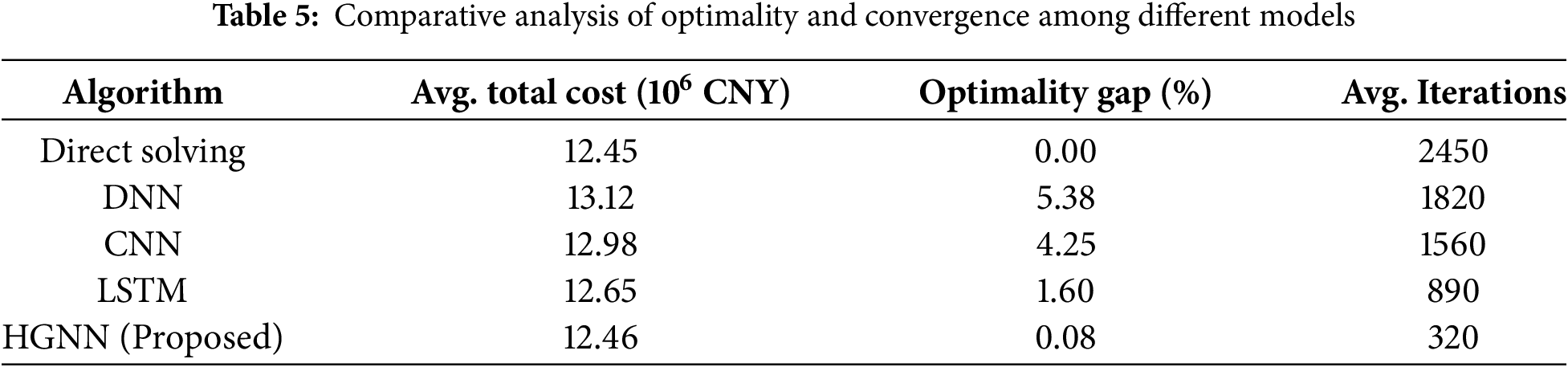
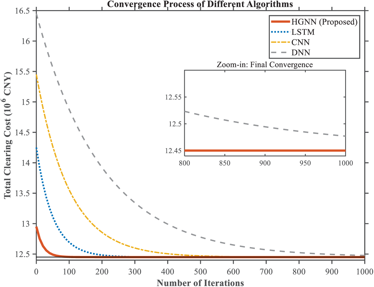
Figure 7: Comparison of convergence behavior and solution optimality among HGNN and baseline models

The HGNN model significantly reduces computation time, validating its real-time capability and engineering feasibility in multi-regional spot market joint clearing scenarios, and providing an efficient intelligent computation approach for electricity market clearing.

4.4 Scalability Analysis on Large-Scale Systems

Clarification on Market Scale and Computational Complexity We believe that the computational scale of the electricity spot market clearing problem depends primarily on the density of market participants (generation-side and demand-side entities) and the number of integer variables they generate, rather than merely the number of administrative regions (provinces). The Heterogeneous Graph Neural Network (HGNN) proposed in this paper aims to capture the complex associations between micro-entities (units/loads) and macro-structures. The nodes of the graph include not only provinces but, more centrally, a large number of “generator nodes” and “load nodes”. Therefore, even if the number of regions is limited, as long as the number of internal participating entities is large or their resource optimization requirements are sufficiently complex, it constitutes a severe test for solver efficiency and HGNN pre-identification capabilities.

Scalability Analysis To empirically prove the robustness and scalability of the proposed method, we expanded the generation capacity and demand-side load scale in the original case study by 100 times, simulating a giant market trading environment. As shown in the Fig. 8, the clearing trends after scaling up are highly consistent with the original analysis. For example, Region 1 continues to exhibit power export behavior due to its low-price advantage, and Region 2 continues to alleviate supply and demand pressure by importing power during peak hours. This demonstrates that the method maintains the accuracy and superiority of its clearing logic when processing larger data capacities. Although the scale of electricity processed by the system increased by 100 times, the HGNN-assisted method was still able to complete the solution within a reasonable time, further confirming that this method has significant advantages over traditional direct solving strategies when dealing with large-scale search spaces.

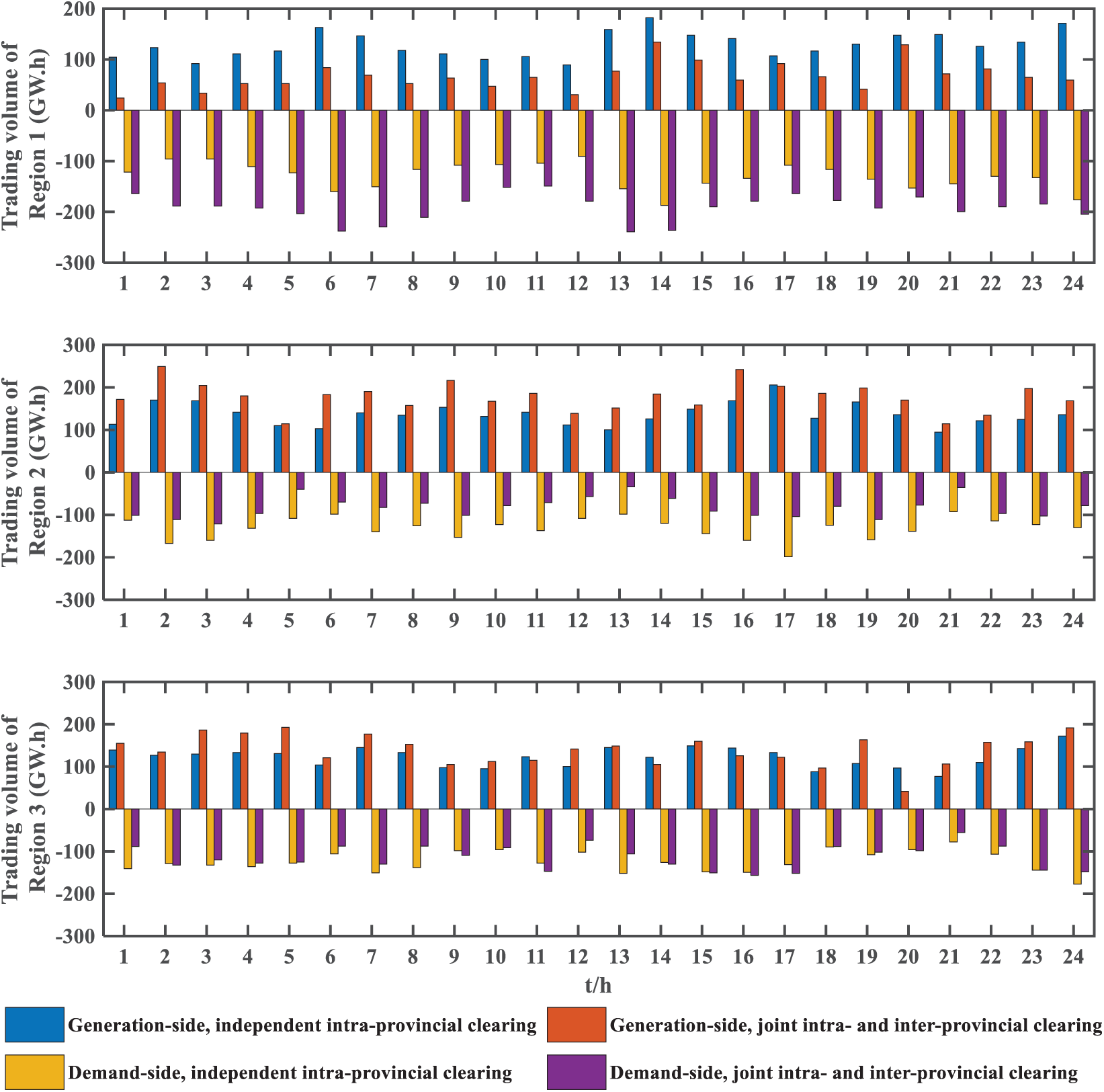
Figure 8: Clearing results of the three regions under the large-scale market scenario (100× scale)

4.5 Performance under Extreme Scenarios

To evaluate model robustness under rare system states, an extreme test set was constructed incorporating N-2 cascading contingencies (simultaneous disconnection of two transmission lines). These scenarios induce severe topological changes absent from the offline training dataset, representing “unseen extreme” conditions. In the experiment, 50% of the standard test samples were replaced with high-risk N-2 contingencies. The performance of the proposed HGNN was benchmarked against the traditional Direct Solving method and a Deep Neural Network (DNN) model, as summarized in Table 6.

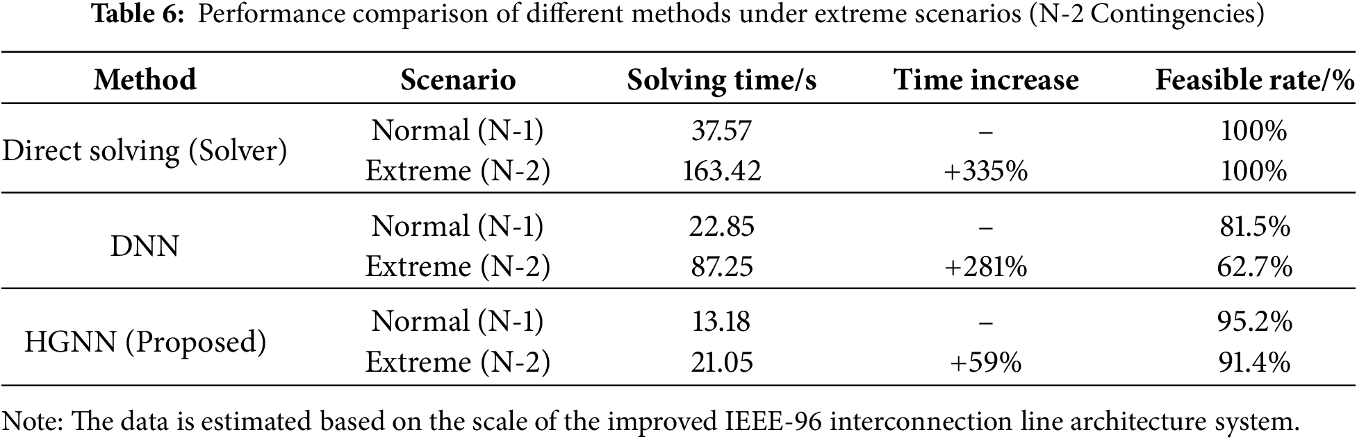
Computational Efficiency: Under N-2 constraints, the traditional solver’s computation time increased by over 300% (37 s to 163 s) due to the exponential complexity of the branch-and-bound search within constricted feasible regions. Conversely, the HGNN maintained real-time viability (~21 s) with only a marginal time increase (+59%). Generalization Capability: The DNN’s feasible solution rate declined significantly (81.5% to 62.7%) when facing unseen topologies, indicating a limited capacity to extract features from structural mutations. In contrast, the HGNN leveraged its topology-aware architecture to maintain a high feasible rate (91.4%), validating its robustness against extreme system faults.

4.6 Generalization Assessment on Unseen Scenarios

Traditional Euclidean-based methods (e.g., CNN, DNN) inherently struggle with structural variations in market configurations. To evaluate the generalization capability of the proposed HGNN under unseen topologies, a comparative experiment was conducted using a test set characterized by “topological mutations.” Specifically, the model was trained on the benchmark topology but tested on datasets containing 0% to 50% “unseen topology samples,” which simulated severe inter-provincial tie-line faults (e.g., double-circuit line outages) absent from the training phase. The identification accuracy and solving time of CNN, DNN, and HGNN were compared, with results detailed in Table 7.

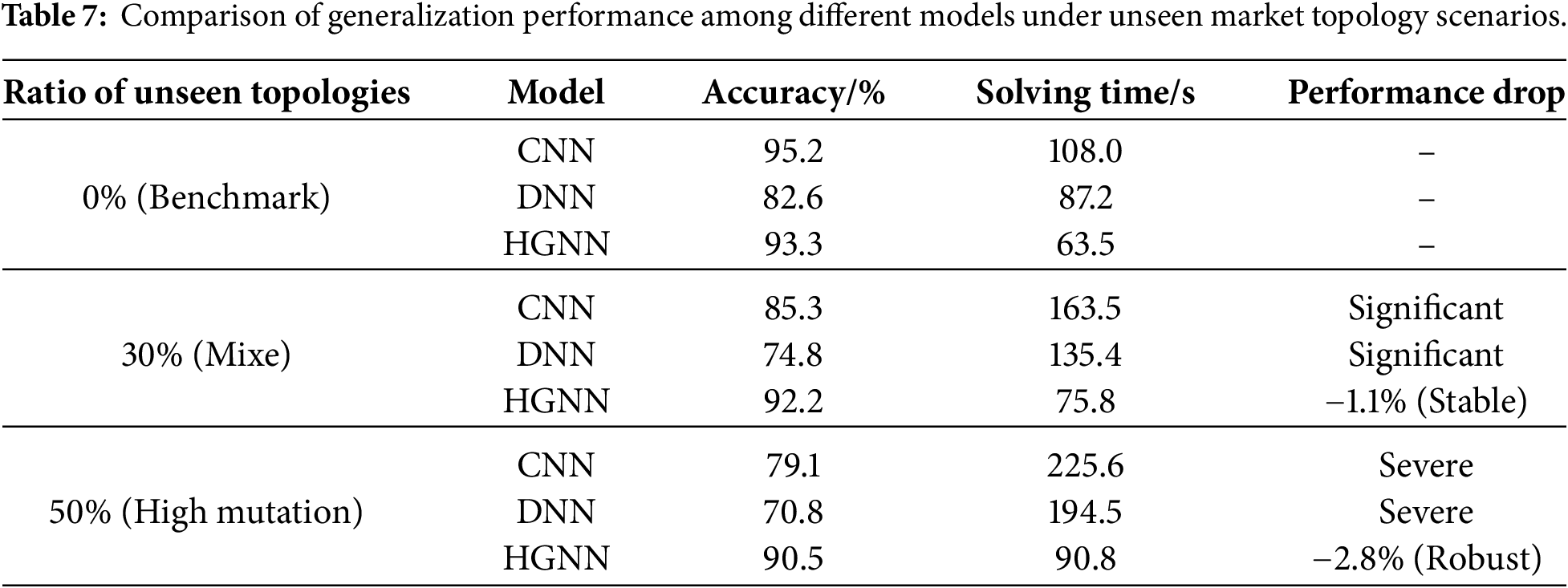
The results indicate a sharp contrast in model adaptability. As the proportion of unseen topologies increases to 50%, non-graph models (CNN and DNN) exhibit significant performance degradation, with accuracy dropping by 16.1% and 11.8%, respectively, alongside a marked increase in computational time. This failure stems from their reliance on fixed-dimensional vectors or grid-based features, which cannot accommodate structural shifts. Conversely, the HGNN demonstrates superior robustness, maintaining over 90% accuracy with a marginal decline (<3%) and stable solving efficiency. This resilience is attributed to the inductive learning capability of the graph architecture, which infers market behaviors based on nodal connectivity relationships rather than memorizing fixed training patterns, thereby effectively handling unseen physical configurations.

4.7 Scalability and Computational Efficiency Analysis

To evaluate scalability, the experimental scope was expanded from the medium-scale benchmark (73 nodes) to a large-scale IEEE 300-node system. Figs. 6 and 9 illustrate the computational performance across varying scales.

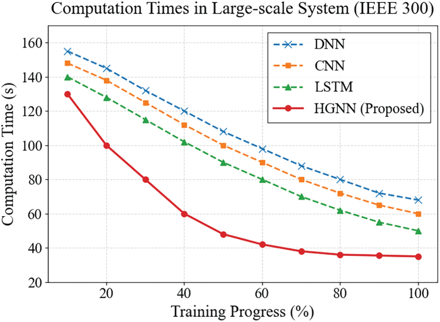
Figure 9: Computation times in large-scale system (IEEE 300)

1.   Computational Time Comparison: In the medium-scale scenario (Fig. 6), the HGNN reduces computation time from ~37 s (traditional solver) to ~13 s, showing a moderate advantage over DNN and CNN models. However, this superiority is significantly amplified in the large-scale system (Fig. 9). While DNN and CNN models suffer from parameter explosion, resulting in computation times exceeding 60 s due to slower convergence, the HGNN maintains a stable time of approximately 35 s. This represents a substantial 45% reduction compared to the DNN baseline, highlighting its efficiency in high-dimensional environments.

2.   Dominant Factors for Improvement: The scalability advantage of the HGNN is driven by its unique structural properties. Unlike DNNs and CNNs, which process systems as flattened vectors or grids and often discard topological dependencies, the HGNN leverages topology awareness to perform message passing directly on graph structures. This mechanism effectively captures the inherent sparsity and non-Euclidean coupling constraints of large-scale power grids, allowing for precise pruning of the search space. Furthermore, the parameter-sharing nature of graph convolutions ensures that model complexity relies on feature dimensionality rather than node count, preventing the linear scaling of computational cost and overfitting risks typical in large-scale optimization.

5  Conclusion

The proposed joint clearing method leverages the structural learning capability of HGNN to efficiently address large-scale optimization problems. Case studies demonstrate that joint clearing enhances inter-provincial resource complementarity, improves cross-provincial power allocation efficiency, and significantly reduces computation time. The method exhibits strong real-time performance and scalability, offering valuable insights for intelligent clearing in future large-scale electricity spot markets.

Acknowledgement: This paper was completed with the hard help of every author.

Funding Statement: This work is supported by Beijing Power Exchange Center Co., Ltd. under the Project “Inter-provincial and intra-provincial joint trading clearing technology supporting large-scale participation of diverse market entities” (Project No. SGJY0000JSJS2400013).

Author Contributions: The authors confirm contribution to the paper as follows: study conception and design: Shijie Ji, Shuya Lei; data collection: Lan Ren; analysis and interpretation of results: Renjie Wei, Ning Yang; draft manuscript preparation: Yishen Wang. All authors reviewed the results and approved the final version of the manuscript.

Availability of Data and Materials: Due to the nature of this research, participants of this study did not agree for their data to be shared publicly, so supporting data is not available.

Ethics Approval: Not applicable.

Conflicts of Interest: The authors declare no conflicts of interest to report regarding the present study.

References

1. Guo H, Davidson MR, Chen Q, Zhang D, Jiang N, Xia Q, et al. Power market reform in China: motivations, progress, and recommendations. Energy Policy. 2020;145:111717. doi:10.1016/j.enpol.2020.111717. [Google Scholar] [CrossRef]

2. Feng Y, Lin J, Song F, Ho MS. Performance and challenges of power sector reform in China since 2015. iScience. 2025;28(10):113461. doi:10.1016/j.isci.2025.113461. [Google Scholar] [CrossRef]

3. Redondo JM, Olivar G, Ibarra-Vega D, Dyner I. Modeling for the regional integration of electricity markets. Energy Sustain Dev. 2018;43:100–13. doi:10.1016/j.esd.2017.12.003. [Google Scholar] [CrossRef]

4. Bjarghov S, Löschenbrand M, Ibn Saif AUN, Alonso Pedrero R, Pfeiffer C, Khadem SK, et al. Developments and challenges in local electricity markets: a comprehensive review. IEEE Access. 2021;9:58910–43. doi:10.1109/ACCESS.2021.3071830. [Google Scholar] [CrossRef]

5. Zhang C, Zhao Q, Ye Y, Chen Z. Design and empirical research on cross-provincial and cross-regional power transmission pricing mechanism adapted to marketized trading in China. Procedia Comput Sci. 2024;242(3):332–9. doi:10.1016/j.procs.2024.08.220. [Google Scholar] [CrossRef]

6. Yue H, Zhang Y, Guo J, Hu Y, Wei C, Jia H, et al. Analysis and construction of evaluation index system of inter-provincial electricity spot markets. Glob Energy Interconnect. 2024;7(6):697–706. doi:10.1016/j.gloei.2024.11.001. [Google Scholar] [CrossRef]

7. Zeng L, Du W, Zhao L, Chen S. An inter-provincial coordinate model under renewable portfolio standards policy based on tradable green certificate options trading. Renew Energy. 2024;234(6):121202. doi:10.1016/j.renene.2024.121202. [Google Scholar] [CrossRef]

8. Wang M, Tan Z, Ma Z, Zhong H, Hu C, Luo Z, et al. Inter-provincial electricity spot market model for China. In: Proceedings of the 2020 IEEE/IAS Industrial and Commercial Power System Asia (I&CPS Asia); 2020 Jul 13–15; Weihai, China. doi:10.1109/ICPSAsia48933.2020.9208589. [Google Scholar] [CrossRef]

9. Tao S, Tan Z, Yang C, Yan Z, Cheng H. Path-aware market clearing model for inter-regional electricity market via redundancy elimination. J Mod Power Syst Clean Energy. 2024;12(6):1980–92. doi:10.35833/mpce.2023.000962. [Google Scholar] [CrossRef]

10. Gao C, Shi S, Yuan M, Tan H, Kang N. Design and optimal clearing model of inter-regional and inter-provincial power trading mechanism considering network constraints. E3S Web Conf. 2021;256(7):01004. doi:10.1051/e3sconf/202125601004. [Google Scholar] [CrossRef]

11. Zhang Y, Zhao X, Yuan H, Yu Y, Yan Z, Zhang K. Key market mechanisms for cross-regional tradings in the electricity market: insights from theory and real-world implementations. IEEE Access. 2024;12(7):97309–31. doi:10.1109/ACCESS.2024.3428310. [Google Scholar] [CrossRef]

12. Cepeda M. Assessing cross-border integration of capacity mechanisms in coupled electricity markets. Energy Policy. 2018;119(2):28–40. doi:10.1016/j.enpol.2018.04.016. [Google Scholar] [CrossRef]

13. Delikaraoglou S, Morales JM, Pinson P. Impact of inter- and intra-regional coordination in markets with a large renewable component. IEEE Trans Power Syst. 2016;31(6):5061–70. doi:10.1109/TPWRS.2016.2530981. [Google Scholar] [CrossRef]

14. Glachant JM. The achievement of the EU electricity internal market through market coupling. In: RSCAS working papers. Fiesole, Italy: European University Institute; 2010. [Google Scholar]

15. Ukoba K, Olatunji KO, Adeoye E, Jen TC, Madyira DM. Optimizing renewable energy systems through artificial intelligence: review and future prospects. Energy Environ. 2024;35(7):3833–79. doi:10.1177/0958305x241256293. [Google Scholar] [CrossRef]

16. Stecyk A, Miciuła I. Harnessing the power of artificial intelligence for collaborative energy optimization platforms. Energies. 2023;16(13):5210. doi:10.3390/en16135210. [Google Scholar] [CrossRef]

17. Liu S, Wu C, Zhu H. Graph neural networks for learning real-time prices in electricity market. arXiv:2106.10529. 2021. [Google Scholar]

18. Liao W, Bak-Jensen B, Pillai JR, Wang Y, Wang Y. A review of graph neural networks and their applications in power systems. J Mod Power Syst Clean Energy. 2022;10(2):345–60. doi:10.35833/MPCE.2021.000058. [Google Scholar] [CrossRef]

19. Dolányi M, Bruninx K, Toubeau JF, Delarue E. Capturing electricity market dynamics in strategic market participation using neural network constrained optimization. IEEE Trans Power Syst. 2024;39(1):533–45. doi:10.1109/TPWRS.2023.3242356. [Google Scholar] [CrossRef]

20. Dvorkin V, Fioretto F. Price-aware deep learning for electricity markets. arXiv:2308.01436. 2023. [Google Scholar]

21. Pagnier L, Ferrando R, Dvorkin Y, Chertkov M. Machine learning for electricity market clearing. arXiv:2205.11641. 2022. [Google Scholar]