Stackelberg-Nash Game Based Collaborative Optimal Low-Carbon Scheduling of Multiple Integrated Multi-Energy Systems via Peer-to-Peer Trading

1  Introduction

The low-carbon and sustainable transformation of traditional energy systems [1] is driving the evolution of traditional energy architectures from a decentralized, independent operation mode to a highly collaborative, efficiently coordinated and intelligent form [2]. Integrated multi-energy systems (IMES) have become a key technical solution in this transformation process, as they can realize the coordinated control of multi-energy flows including electricity, heat, cooling and natural gas under a unified architecture [3]. Through the coordinated optimization of multi-energy loads, IMES can effectively improve comprehensive energy utilization efficiency and accommodate the grid integration demand of high-penetration renewable energy systems (RES) [4]. However, the system complexity induced by multi-energy coupling [5], the stochastic volatility of renewable energy output, and the interest conflicts among multi-stakeholders in game interactions have posed severe challenges to the optimal scheduling and economic operation of IMES.

To address these challenges, scholars have carried out extensive research on the optimal operation of IMES. Work [6] proposed a stochastic gradient-enhanced distributionally robust optimization framework. Simulation results based on annual actual operation data showed that the framework could significantly improve the coordination ability of IMES, up to a 25% cost reduction during peak demand periods, and significantly outperformed conventional optimization systems. Reference [7] proposed a scheduling method of multi-level game for distribution network-microgrid-flexible load systems, which enhanced optimization efficiency, promoted photovoltaic (PV) accommodation [8], improved the overall economic performance of the system by 24.5%, and increased the benefits of all stakeholders. Reference [9] proposed a Stackelberg game framework for operational optimization of multi-microgrid systems, which promoted PV accommodation, enhanced system profitability, and increased the benefits of all stakeholders. Work [10] proposed a three-layer optimal scheduling model. The model was solved via Karush-Kuhn-Tucker (KKT) conditions for each layer of the game, the proposed method enables a substantial reduction in system operation costs and carbon emissions, and delivers a mutually beneficial equilibrium for all stakeholders. Reference [11] focused on the collaborative optimization of regional integrated energy systems, and solved the model with alternating direction method of multipliers (ADMM) algorithm. Case results showed that the proposed mechanism reduced the operational costs of regional integrated energy systems by 4.97% and carbon emissions by 0.81%, which corroborates the effectiveness of multi-energy sharing mechanisms for advancing the economic performance and low-carbon attributes of integrated energy systems. Reference [12] proposed an optimal operation strategy based on a bi-level Stackelberg game framework for multi-regional integrated energy systems. Results showed that the strategy reduced the operational cost of each region by up to 27.7%, significantly improved the renewable energy utilization rate of each region, and achieved a prominent carbon emission reduction effect. Work [13] proposed a shared energy storage (SES) optimization model for IMES. Simulation results showed that the proposed method reduced the total cost and energy cost of the system by 14.461% and 22.925%, respectively, which fully validated the effectiveness of the model.

However, these studies have limitations in solving the collaborative optimization of multi-IMES economic operation and low-carbon development, which severely restrict the full exploitation of the systems’ operational potential. Most existing studies are confined to single-scale game modeling and optimization. A number of studies only focus on the robust optimal operation of a single IMES, while neglecting the interest conflicts and collaboration potential among multiple stakeholders, and thus fail to establish a unified bi-level collaborative optimization framework [14]. These studies cannot achieve the deep coupling between the internal Stackelberg game of a single IMES and the coalition Nash bargaining game among multiple IMES, making it difficult to simultaneously balance local interest equilibrium and optimal allocation of global cross-system resources, as evidenced by the work in [15]. Meanwhile, the synergy between low-carbon technologies and market mechanisms remains insufficient. Most existing studies merely focus on the optimization of a single low-carbon technology or DR mechanism [16], and fail to realize full-dimensional collaborative optimization of low-carbon technologies in conjunction with price-based DR and peer-to-peer (P2P) electricity trading mechanisms [17]. As a flexibility regulation resource of IMES, price-based DR guides end-users to adjust their electricity and heat consumption behaviors through time-of-use (ToU) dynamic pricing, which can effectively smooth the load peak-valley difference, improve the accommodation capacity of renewable energy, and reduce the system operation cost and carbon emissions. This paper integrates the price-based DR mechanism into the Stackelberg game framework, and realizes the coordinated optimization of system low-carbon operation and multi-stakeholder benefit balance. Accordingly, they cannot fully unlock the synergistic potential of IMES in reducing both economic costs and carbon emissions. In addition, the revenue distribution mechanism of the multi-IMES alliance is deficient in targeted incentives and fairness guarantees. The traditional Nash bargaining model widely adopted in existing cooperative game studies fails to correlate revenue distribution outcomes with the actual comprehensive contribution of each participant. This deficiency fails to provide an effective positive incentive for alliance members, and may even jeopardize the long-term stable operation of the multi-IMES alliance. Furthermore, existing algorithms exhibit poor adaptability to the bi-level coupled game model. For the high-dimensional nonlinear and non-convex optimization problems introduced by the hierarchical game structure of IMES, traditional heuristic algorithms have inherent drawbacks, including insufficient global search capability [18] and unsatisfactory robustness [19] in high-dimensional space. Meanwhile, there is a lack of hierarchical distributed solution strategies tailored to the bi-level game structure, which makes it difficult to strike a balance between solution accuracy and computational efficiency in practical engineering applications.

To fill the abovementioned research gaps, this paper proposes a collaborative optimization framework for integrated multi-energy systems based on the Stackelberg-Nash game, which realizes the deep synergy of hydrogen blending technology [20], demand response (DR) mechanisms, and P2P electricity trading. Specifically, the upper layer addresses the optimal interaction between energy pricing and DR through the Stackelberg game between the IMES operator (IMESO) and LAs; the lower layer realizes the maximization of total alliance revenue and fair revenue distribution through the Nash bargaining game [21] among multiple IMES based on P2P electricity trading. Meanwhile, low-carbon technologies are fully integrated into the optimization framework, and a hierarchical solution strategy combining covariance matrix adaptation evolution strategy (CMA-ES) and ADMM is designed to efficiently solve the proposed model [22]. Simulation calculation results provide sufficient verification for the effectiveness of the proposed method in reducing carbon emissions, which provides a feasible and superior solution for the efficient and clean operation of regional IMES.

In summary, this paper makes the following contributions to the existing research:

(1)   A unified bi-level Stackelberg-Nash game [23] collaborative optimization framework is constructed, which simultaneously balances the local interest equilibrium and the optimal allocation of global cross-system resources. The CMA-ES algorithm is adopted for the high-dimensional nonlinear non-convex problem of the upper-level Stackelberg game to realize efficient global optimization, and ADMM is used to solve the lower model [24], which balances the solution accuracy and computational efficiency;

(2)   An IMES architecture integrating low-carbon technologies including the hydrogen blending system (HBS), water electrolysis (EL) for hydrogen production, and carbon capture system (CCS) is established [25], which achieves the full-dimensional collaborative optimization of low-carbon technologies, price-based DR and P2P electricity trading mechanisms, and unlocks the synergistic potential of IMES in reducing economic costs and carbon emissions;

(3)   A revenue distribution mechanism linked to the actual comprehensive contribution of each participant is constructed [26], which forms an effective positive incentive for alliance members and guarantees the long-term stable operation of the multi-IMES alliance.

This paper is organized as follows. Section 2 presents the system architecture and core optimization objectives of single IMES, the multiple IMES alliance and the overall collaborative framework. Section 3 constructs IMES game model, including Stackelberg game between the IMESO and LA, and Nash bargaining game for the multiple IMES alliance. Section 4 introduces the hierarchical model solving algorithm, and elaborates the detailed solving steps for the upper and lower-layer game models, respectively. Section 5 carries out the case study, including the basic data of the case. Finally, the last section summarizes the research conclusions of this paper.

2  Structure of the Game Model

2.1 Structure of IMES

Stackelberg-Nash game model framework is shown in Fig. 1. Among them, IMES is responsible for energy production, equipment scheduling and price setting. Each IMES consists of a RES generator, CHP, battery energy storage systems (BESS), gas boiler (GB), EL, CCS and power to gas (PTG) [27]. The hydrogen produced by the surplus renewable energy is mixed with carbon dioxide to produce methane, which is used as a gas fuel for other IMES. LA manages transferable power loads and reduces heat loads, and responds to IMESO pricing strategy through DR.

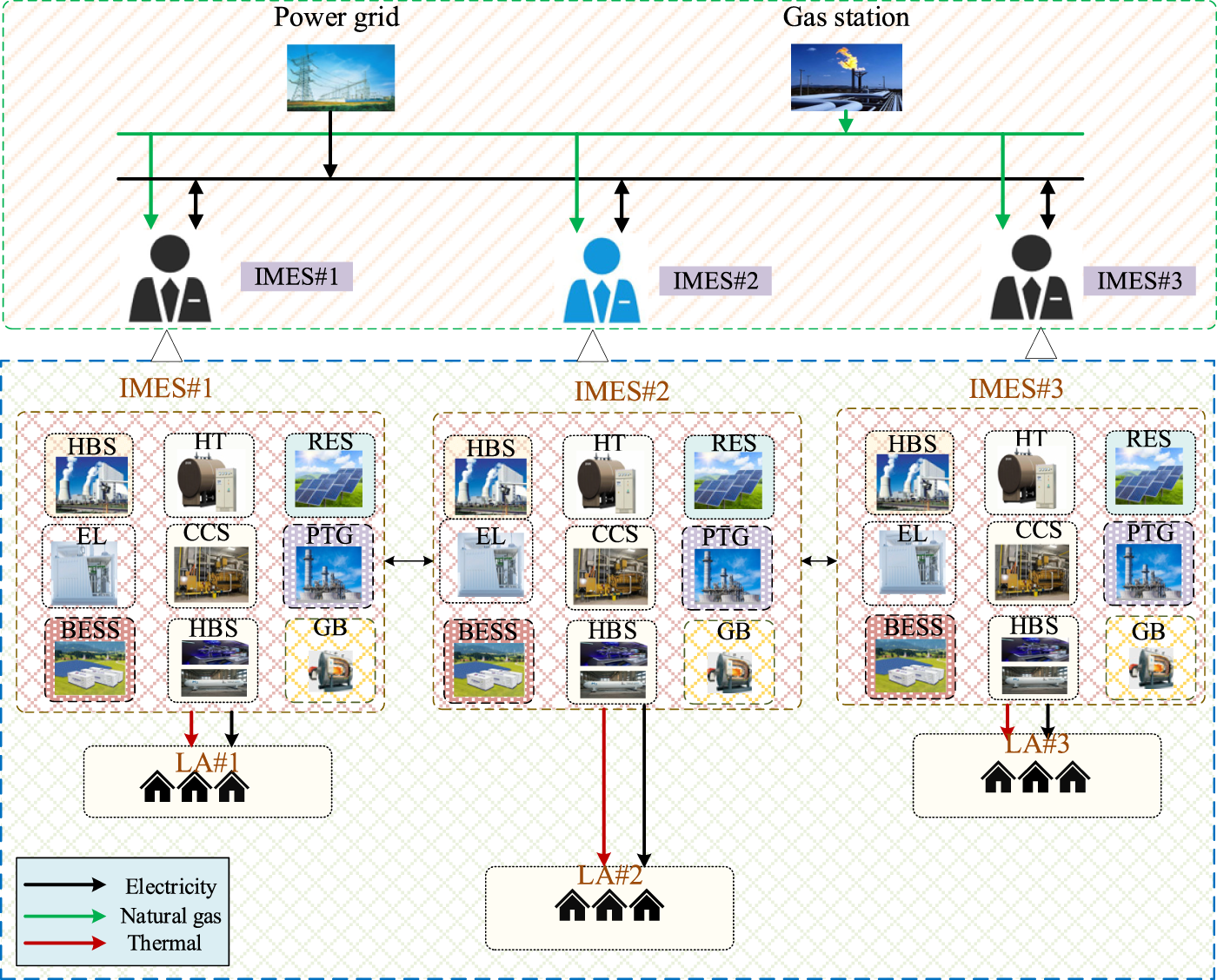
Figure 1: Structure of multiple IMES.

RES is mainly responsible for providing clean power. CHP and GB reduce carbon emissions from natural gas combustion via hydrogen blending; EL consumes surplus electricity from RES to produce hydrogen; BESS stabilizes RES fluctuation and realizes power time shift. CCS captures indirect carbon emissions from HBS and electricity purchase. HBS and CCS can form a low-carbon technology combination with complementary advantages, which can reduce carbon emissions from emission sources and end-of-pipe treatment. HBS replaces natural gas with hydrogen, which enables direct carbon emission reduction during the fuel combustion phase. Meanwhile, it can convert surplus renewable electricity into storable hydrogen fuel, effectively addressing the curtailment loss problem of new energy power generation. As an end-of-pipe emission reduction technology, CCS can capture carbon emissions generated from fuel combustion and grid-purchased electricity, thus possessing carbon abatement capability. The captured carbon dioxide can also be recycled through methanation reaction to produce natural gas, thereby constructing a closed-loop carbon cycle system. This system can not only reduce the procurement cost of natural gas but also cut down the expenditure on carbon emission penalties.

2.2 Low-Carbon Scheduling Framework Based on Bi-Level Game

The optimal scheduling of IMES needs to solve the two core problems of multi-agent conflict of interest and multi-objective collaborative optimization. From the perspective of participating agents, the system involves three types of decision-making subjects: IMESO, LA and multiple IMES alliance. IMESO pursues profit maximization, LA focuses on user energy surplus, and multiple IMES needs to achieve fair cooperative income distribution. From the objective perspective, consider the improvement of economic benefits and the reduction of carbon emissions based on meeting the electricity/thermal load demand. It is difficult for a single optimization framework to balance multi-objective priorities.

Therefore, based on the hierarchical logic of local decision-making-global coordination, this paper constructs a bi-level Stackelberg-Nash game model [28]. The upper level focuses on the coordination of interests within IMES, solves the interaction problem between IMESO pricing and LA load response, and accommodates the local scheduling characteristics of DR; the lower level focuses on the optimization of cooperation among multiple IMES, solves the coordination problem of alliance revenue maximization and fair distribution, and adapts to the global resource allocation requirements of P2P electricity trading [29]. The equilibrium result of the upper game will be used as the input parameter of the lower game, which provides local constraints for the calculation of P2P transaction scale and the optimization of equipment operation strategy of multiple IMES alliance. P2P transaction results of the lower game will reversely correct the external interaction costs of the upper level. The framework of bi-level model is shown in Fig. 2.

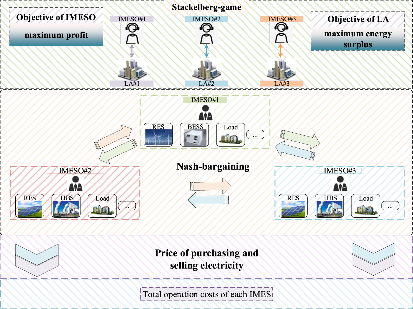
Figure 2: Structure of bi-level Stackelberg-Nash game model.

3  IMES Game Model

3.1 Stackelberg Game

In the price-based DR framework, this paper constructs a single-leader multi-follower Stackelberg game model between IMESO and multiple LAs. Among them, IMESO, as the leader of the game, takes the lead in formulating the dynamic DR electricity price and heat price in each scheduling period with the goal of maximizing its own operating revenue; LAs, as the followers of the game, make the optimal electric load and heat load adjustment decisions according to the price strategy issued by IMESO, with the goal of maximizing the consumer surplus of end-users. The game equilibrium is achieved when the leader’s pricing strategy and the followers’ load response strategy reach the optimal state at the same time.

3.1.1 IMESO Model

(1) Objective function of IMESO

IMESO incorporates LA’s optimal load response into its objective function to optimize DR electricity/heat price. The objective function is shown

maxUIMESO=RDR−CCO2−CEIC−COP(1)

where RDR is the energy sales revenue after DR; CEIC is the external interaction cost; COP represents the cost of operation; CEIC represents the external interaction cost; CCO2 means the carbon penalty cost.

The revenue from IMESO selling electricity and thermal after DR is shown

RDR=∑t=1T[πe,DR(t)⋅Pe,DR(t)+πh,DR(t)⋅Qh,DR(t)](2)

where πe,DR(t) and πh,DR(t) represent the electricity and thermal price after DR, respectively; Pe,DR(t) and Qh,DR(t) represent the electric and thermal power sold by IMESO to LA after DR, respectively.

The operation and maintenance costs are as follows

COP=∑t=1T⁡{COP,CHP⋅PCHP(t)+COP,RES⋅PRES(t)+COP,BESS⋅[PBESS,dis(t)+PBESS,cha(t)]+COP,EL⋅PEL(t)+COP,CCS⋅PCCS(t)+Ccut⋅PRES,cut(t)+COP,GB⋅QGB(t)}(3)

where COP,RES, COP,GB, COP, CHP, COP,BESS, COP,CCS and COP,EL sequentially represent the operation costs of RES, GB, CHP, BESS, CCS and EL; Ccut refers to the unit cost of renewable energy abandonment; PRES(t), PCCS(t), PCHP(t), and PEL(t) denote the output power of RES, CCS, CHP and EL in time slot t, respectively; QGB(t) is the thermal power output from the HBS-GB; PBESS,dis(t) and PBESS,cha(t) are the discharging and charging power of the BESS in time slot t, respectively; PRES,cut(t) stands for the renewable energy power curtailed in time slot t.

The calculation of external interaction cost is given

CEIC=∑t=1T   πgrid,buy(t)⋅PG,buy(t)−πgrid,sell(t)⋅PG,sell(t)+πgas,buy(t)⋅Vgas,buy(t)(4)

where πgrid,buy(t) is ToU purchase electricity price from the grid; πgrid,sell(t) represents the on-grid price. PG,buy(t) and PG,sell(t) denote the purchase and sale of electricity quantity from the grid, respectively; πgas,buy(t) is the purchase price of gas; Vgas,buy(t) represents the volume of gas purchased.

To ensure the economic rationality of the price-based DR mechanism, the electricity price after DR formulated by IMESO must be between the grid feed-in price and the grid ToU purchase price, so as to ensure that IMESO has a reasonable profit margin, and at the same time, the end-users’ electricity cost is lower than the cost of directly purchasing electricity from the utility grid. The electricity price constraint is shown

πgrid,sell(t)<πe,DR(t)<πgrid,buy(t)(5)

The heat price after DR needs to be within the preset upper and lower limits to avoid excessive heat price fluctuations affecting the basic heat demand of end-users. The thermal price constraint is expressed

πh,min(t)<πh,DR(t)<πh,max(t)(6)

where πh,min(t) and πh,max(t) represent the minimum thermal price and the maximum thermal price, respectively.

IMESO needs to pay a penalty cost for excessive carbon emissions. The calculation is shown

CCO2=∑t=1T{πCO2,trad⋅max[MCO2,AC(t)−MCO2,Quo(t),0]}(7)

where πCO2,trad represents the penalty cost coefficient of carbon dioxide, and MCO2,AC(t) represents the actual carbon dioxide emissions at time t; carbon dioxide emission quota at MCO2,Quo(t); formula function: when the actual level of carbon emissions breaks through the pre-allocated carbon emission quota, the penalty cost needs to be paid; if it is not exceeded, there is no penalty, so as to encourage IMES to reduce emissions.

The actual net carbon emissions are

MCO2,AC(t)=MCO2,CHP(t)+MCO2,GB(t)+MCO2, grid(t)−ηCCS⋅MCO2, abs(t)(8)

where MCO2,CHP(t) and MCO2,GB(t) represent the carbon emissions from CHP and GB combustion, respectively; MCO2, grid(t) is the carbon emission from the grid; MCO2,abs(t) represents the carbon absorbed by CCS; ηCCS is the capture efficiency of CCS.

Carbon emissions are obtained based on the carbon emission factors of natural gas combustion per unit volume, as shown

MCO2,CHP(t)=Mgas,CHP(t)ρgas⋅εgas(9)

MCO2,GB(t)=Mgas,GB(t)ρgas⋅εgas(10)

where ρgas denotes the density of natural gas and εgas denotes the mass of carbon dioxide produced per cubic metre of natural gas burned, respectively; Mgas,GB(t) and Mgas,CHP(t) represent the mass of natural gas consumed by GB unit and CHP unit, respectively.

The electricity purchased by external interaction is mainly from thermal power plants, and the calculation of carbon emissions is given

MCO2, grid(t)=PG,buy(t)⋅εth⋅Δt(11)

where εth represents the carbon dioxide emission density.

Carbon emission quota is calculated as follows

MCO2,Quo(t)=PCHP(t)⋅Δt⋅μeCHP+QCHP(t)⋅Δt⋅μhCHP+QGB(t)⋅Δt⋅μhGB+PG,buy(t)⋅Δt⋅μegrid(12)

where μ∗ represents the carbon emission allowance coefficient of the corresponding energy production link.

(2) System Operation Constraints

The equipment scheduling decision of IMESO must meet the equipment safe operation constraints and energy supply and demand balance constraints.

RES output constraints are as shown

PRES(t)=PRES,av(t)−PRES,cut(t)(13)

0≤PRES,cut(t)≤PRES,av(t)(14)

where PRES,av(t) is the maximum available power of RES.

Equipment operation power and ramp constraints are as shown

0≤Pδ(t)≤Pδmax,δ∈{CHP,GB,BESS}(15)

Pεdown≤Pε(t+1)−Pε(t)≤Pεup,ε∈{CHP,GB,BESS}(16)

where Pδ(t) is the operating power of equipment δ; Pδmax is the rated maximum power of the equipment; Pεup and Pεdown are the upper and lower ramp limits of the equipment, respectively.

Main grid interaction power constraints are as given

0≤PG,sell(t)≤Pgrid,sellmax(17)

0≤PG,buy(t)≤Pgrid,buymax(18)

where PG,buymax and PG,sellmax are the maximum upper limits of power sold to and purchased from the grid, respectively.

BESS operation constraints are as shown

EBESS(t+1)=EBESS(t)+PBESS,cha(t)⋅Δt⋅ηBESS,cha−PBESS,dis(t)⋅ΔtηBESS,dis(19)

where EBESS(t) represents the energy storage capacity of BESS; ηBESS,cha and ηBESS,dis are charge-discharge efficiency, respectively.

0≤PBESS,cha(t)≤PBESSmax⋅uBESS(t)(20)

where uBESS(t) is a 0–1 binary variable characterizing the charging and discharging status of BESS.

0≤PBESS,dis(t)≤PBESSmax⋅[1−uBESS(t)](21)

SOCBESSmin≤EBESSEBESS,rated≤SOCBESSmax(22)

where SOCBESSmin and SOCBESSmax denote the lower and upper limits of SOC, respectively; EBESS,rated is the rated capacity of BESS. In this paper, EBESS,rated is set to 4000 kWh, SOCBESSmin and SOCBESSmax are set to 0.2 and 0.9, respectively.

EBESS(start)=EBESS(end)(23)

CCS operation constraints are as follows

{VL(t+1)=VL(t)+VL,in(t)−VL,out(t)VR(t+1)=VR(t)+VR,in(t)−VR,out(t)VL,in(t)=MCO2,abs(t)⋅ηCCSρco2⋅γVR,out(t)=MCO2,use(t)ρco2⋅γVL(t)+VR(t)=VtankmaxMCO2,use(t)=PCCS,OP(t)⋅ΔtecarPCCS(t)=PCCS,OP(t)+PCCS,F(t)(24)

where VL(t) and VR(t) are the volume of lean liquid and rich liquid of CCS, respectively; MCO2,abs(t) is the carbon absorption of CCS; ρco2 is the density of carbon dioxide; γ is the carbon absorption ratio of the absorption liquid; Vtankmax is the maximum volume of HT; MCO2,use(t) refers to the mass of carbon dioxide used for resource utilization; PCCS,F(t) and PCCS,OP(t) denote the fixed and operational power cost of CCS, respectively; ecar is the unit power cost of carbon utilization.

HBS operation constraints are as follows

{PCHP(t)⋅Δt=[MH2,CHP(t)⋅nH2+Mgas,CHP(t)⋅ngas]⋅ηCHPPQCHP(t)⋅Δt=[MH2,CHP(t)⋅nH2+Mgas,CHP(t)⋅ngas]⋅ηCHPTQGB(t)⋅Δt=[MH2,GB(t)⋅nH2+Mgas,GB(t)⋅ngas]⋅ηGBT(25)

where MH2,CHP(t) and Mgas,CHP(t) are the mass of hydrogen and natural gas consumed by CHP, respectively; MH2,GB(t) and Mgas,GB(t) refer to the fuel consumption mass of hydrogen and natural gas for the gas boiler at time t, respectively; ngas and nH2 represent the heating values of gas and hydrogen, respectively; ηCHPP and ηCHPT are the electrical and thermal conversion efficiency of CHP, respectively; ηGBT is the thermal conversion efficiency of GB. The volume ratio of hydrogen blending is set to be less than 20% [30].

Hydrogen tank operation constraints are as expressed

HHT(t+1)=HHT(t)+[MH2,EL(t)−MH2,Me(t)−MH2,GB(t)−MH2,CHP(t)]⋅Δt(26)

where HHT(t) is the hydrogen storage capacity of the hydrogen tank; MH2,EL(t) is the hydrogen production of EL; MH2,Me(t) is the hydrogen consumption for methanation.

MH2,EL(t)=PEL(t)nH2⋅ηEL⋅Δt(27)

where ηEL is the hydrogen production efficiency of EL.

LOHHTmin≤HHT(t)HHT,rated≤LOHHTmax(28)

where LOHHTmin and LOHHTmax are the lower and upper limits of hydrogen storage level, respectively; HHT,rated is the rated capacity of HT. In this paper, HHT,rated is set to 8000 Nm3, LOHHTmin and LOHHTmax are set to 0.1 and 1 respectively.

HHT(0)=HHT(T)(29)

Electric power balance is as follows

PRES(t)+PBESS,dis(t)+PG,buy(t)+PCHP(t)=+PEL(t)+PCCS(t)+Pe,DR(t)+PG,sell(t)+PBESS,cha(t)(30)

Thermal power balance is as follows

QCHP(t)+QGB(t)=Qh,DR(t)(31)

Natural gas balance is as follows

Vgas,GB(t)+Vgas,CHP(t)=Vgas,buy(t)+Vgas,Me(t)(32)

where Vgas,GB(t) and Vgas,CHP(t) are the volume of natural gas consumed by GB and CHP, respectively; Vgas,Me(t) is the volume of natural gas produced by methanation.

CCS carbon absorption constraints are as follows

0≤ηCCS⋅MCO2,abs(t)<MCO2,CHP(t)+MCO2,GB(t)+MCO2, grid(t)(33)

The constraint can be obtained according to Eq. (8).

3.1.2 LA Model

(1) Objective function of LA

The optimization goal of LA is to maximize consumer surplus, that is, the difference between the user’s energy utility and the energy purchase cost. The objective function is shown

maxULA=∑t=1T[fLA(t)−πe,DR(t)⋅Pe,DR(t)−Qh,DR(t)⋅πh,DR(t)]⋅Δt(34)

where the utility function of LA is denoted by fLA(t). It is essentially the maximum total value that LA is willing to pay for the corresponding electricity and heat consumption during this period.

fLA(t)=vePe,DR(t)−ae2Pe,DR2(t)+vhQh,DR(t)−ah2Qh,DR2(t)(35)

where ve and ae are the preference coefficients of electric load utility; vh and ah are the preference coefficients of thermal load utility. In this paper, ve is 2, ae is 0.0004, vh is 1, and ah is 0.00055.

(2) Constraints

Electricity load adjustment range constraint: Limit the maximum adjustment range of electricity load in a single period to avoid large load fluctuations affecting system stability, as shown

Pe,or(t)⋅(1−φe)≤Pe,DR(t)≤Pe,or(t)⋅(1+φe)(36)

where Pe,or(t) is the original electricity load at time t; φe is the maximum transfer ratio of electricity load.

Daily total electricity load conservation constraint: DR only realizes the temporal transfer of load, does not change the user’s total daily electricity consumption, and guarantees the user’s basic electricity demand, as given

∑t=1TPe,DR(t)=∑t=1TPe,or(t)(37)

Thermal load reduction constraint: The heat load can only be reduced but not transferred, and the maximum reduction ratio in a single period does not exceed the set upper limit, as expressed

0≤Qh,cut(t)≤Qh,or(t)⋅φh(38)

Qh,DR(t)=Qh,or(t)−Qh,cut(t)(39)

where Qh,or(t) is the original heat load at time t; Qh,cut(t) is the reduced heat load at time t; φh is the maximum reduction ratio of heat load.

(3) Optimal solution and proof

Game participant set: N={IMESO;LA}, IMESO is the leader of the game and has the first-hand advantage of decision-making; LA is the follower of the game and adjusts its load decision according to the leader’s price strategy.

Strategy space: The strategy space of IMESO is the electricity price and thermal price after DR, that is, SIMESO=πe,DR(t),πh,DR(t), which needs to meet the upper and lower price constraints; the strategy space of follower LA is the electric load and heat load after DR adjustment, that is, SLA={Pe,DR(t),Qh,DR(t)}, which needs to meet the load adjustment constraint.

Revenue function: They are the operating income function of IMESO and the consumer surplus function of LA, respectively. Both sides of the game aim at maximizing their own income.

Proof of non-empty and continuous functions. SIMESO and SLA are linear constraints [i.e., Eqs. (5) and (6), Eqs. (36)–(39)]. The constraints include explicit upper and lower bounds; the corresponding set is bounded; a bounded closed set is a compact set. Meanwhile, the upper bound of a constraint is strictly greater than the lower bound, the non-emptiness of the set can be rigorously proven.

By calculating the first partial derivative and making it to zero, the optimal load strategy of LA is obtained

∂ULA∂Pe,DR(t)=ve−aePe,DR(t)−πe,DR(t)(40)

∂ULA∂Qh,DR(t)=vh−ahQh,DR(t)−πh,DR(t)(41)

Pe,DR∗(t)=ve−πe,DR(t)ae(42)

Qh,DR∗(t)=vh−πh,DR(t)ah(43)

Proof of continuous concave/convex function. The second-order partial derivative and Hessian matrix are used to verify that the objective function of LA is a strictly concave function, are formulated as

∂2ULA∂Pe,DR2(t)=−ae<0(44)

∂2ULA∂Qh,DR2(t)=−ah<0(45)

Hessian matrix is a negative definite matrix, which proves that the objective function of LA has a unique optimal solution.

H(ULA)=[−ae00−ah]≺0(46)

Proof of non-empty and continuous functions. The second-order partial derivative and Hessian matrix are used to verify that the objective function of IMESO is a strictly concave function, as given

∂2UIMESO∂πe,DR2(t)=−2ae(47)

∂2UIMESO∂πh,DR2(t)=−2ah(48)

Proof of continuous concave/convex function. Hessian matrix corresponding to the IMESO objective function is constructed as follows

H(CIMESO)=[−2ae00−2ah]≺0(49)

From Eqs. (44)–(46), since ae>0 and ah>0, the Hessian matrix of the LA’s objective function is negative definite. Therefore, LA’s utility function is strictly concave with respect to Pe,DR(t) and Qh,DR(t). Meanwhile, the feasible strategy set of the LA defined by Eqs. (36)–(39) is non-empty, closed, bounded and convex. Hence, for any given price strategy (πe,DR(t),πh,DR(t)) of IMESO, LA has a unique optimal response. Furthermore, according to Eqs. (42) and (43), which are continuous and single-valued functions of the electricity and heat prices. Substituting Eqs. (42) and (43) into IMESO’s objective function, the leader’s optimization problem can be transformed into a single-level optimization problem with respect to πe,DR(t) and πh,DR(t). From Eqs. (47)–(49), the Hessian matrix of the transformed IMESO objective function is negative definite.

Therefore, the transformed IMESO’s objective function is strictly concave over its feasible price strategy set. Since the price constraints in Eqs. (5) and (6) form a non-empty, closed, bounded and convex feasible set, IMESO has a unique optimal price strategy. Consequently, Stackelberg equilibrium between IMESO and LA exists and is unique.

Proof of uniqueness of Stackelberg–Nash equilibrium. To further prove the uniqueness of the Stackelberg–Nash equilibrium, the hierarchical game is analyzed from the lower-level Nash game and the upper-level Stackelberg decision, respectively.

For any given decision of IMES, the strategy set of each load aggregator is nonempty, compact and convex due to the operational constraints. As shown by the Hessian matrices in Eqs. (44)–(49), the objective function of each participant is strictly concave with respect to its own decision variables. Therefore, each load aggregator has a unique best response. Moreover, the pseudo-gradient mapping of the lower-level Nash game is strictly monotone, or equivalently, the weighted sum of the Hessian matrices satisfies the diagonal strict concavity condition proposed by Rosen. Hence, for any given upper-level decision, the Nash equilibrium among LAs is unique.

Let the unique Nash equilibrium response of the lower-level game be denoted by

x∗=ℛ(p)(50)

where p represents the decision vector of IMES and x∗ denotes the equilibrium response of LAs. Since the lower-level Nash equilibrium is unique, ℛ(⋅) is a single-valued response mapping. Substituting x∗=ℛ(p) into the upper-level optimization problem yields an equivalent single-level problem for IMES. The feasible set of IMES is also nonempty, compact and convex, and its equivalent objective function remains strictly concave with respect to p. Therefore, IMES has a unique optimal decision p∗.

Consequently, the corresponding lower-level Nash equilibrium x∗=ℛ(p∗) is also unique. Thus, the pair (p∗,x∗) constitutes the unique Stackelberg–Nash equilibrium of the proposed hierarchical game.

3.2 Nash Bargaining Model

Based on the optimal operation results of IMES obtained from the upper-level Stackelberg game [31], the lower layer constructs Nash bargaining game model for multi-IMES alliance to optimize IMES P2P power transactions, maximize the total alliance revenue, and according to the comprehensive contribution index of IMES to achieve a fair distribution of income.

3.2.1 Objective Function

The optimization goal of multi-IMES alliance is to maximize the Nash product of the operating income of each IMES alliance minus the independent operating income. As shown in Eq. (51), this objective introduces a bargaining power factor linked to actual contribution and alliance rationality, thereby achieving the Nash bargaining equilibrium.

{max∏i=1N(US,i−UIMESO,i)ωis.t.US,i−UIMESO,i≥0∑i=1Nωi=1(51)

where N is the number of IMES; US,i is the bargaining revenue of the ith IMES after participating in the alliance; UIMESO,i is the maximum revenue of the ith IMES when operating independently; ωi is the comprehensive contribution index of the i-th IMES defined in Eq. (58); the constraint is the individual rationality constraint, that is, the revenue of IMES after participating in the alliance is not lower than the revenue when operating independently.

3.2.2 Constraints

After the introduction of P2P trading, the power balance constraint of each IMES in the alliance needs to include P2P trading terms and is formulated as

PRES(t)++PBESS,dis(t)+PG,buy(t)+PCHP(t)=Pe,DR(t)+PG,sell(t)+PEL(t)+PCCS(t)+PBESS,cha(t)+Pij(t)(52)

where Pij(t) is P2P transaction power from the ith IMES to the jth IMES, positive value for power selling, negative value for power purchasing.

P2P electricity trading meets the following constraints

0≤|Pij(t)|≤Pe,ijmax(53)

Pij(t)=−Pji(t),∀i≠j(54)

where Pe,ijmax is the maximum transaction power between IMES i and j, which is determined by the nominal power of the line; in this paper, Pe,ijmax is set to 10,000 kW. Eq. (54) is the transaction power reciprocity constraint, which ensures that the power sold by IMES i to IMES j is exactly equal to the power purchased by IMES j from IMES i. This constraint explicitly prohibits simultaneous bidirectional power transactions between the same pair of IMES, which would otherwise cause unnecessary line losses, transaction costs and scheduling redundancy.

Transaction electricity price constraint: P2P transaction price needs to be between the main network price and ToU price to ensure that both parties are profitable, as expressed

πgrid,sell(t)≤πij(t)≤πgrid,buy(t)(55)

where πij(t) is P2P transaction electricity price between IMES i and j.

3.2.3 Revenue Distribution Mechanism

To ensure the fairness and rationality of the alliance’s revenue distribution, a comprehensive contribution evaluation index based on the power contribution index and carbon abatement contribution index is proposed in this paper, and integrates it into the Nash bargaining objective function, so that the income distribution is linked to the actual contribution of each IMES.

(1) Power contribution index: Quantify the power supply contribution of IMES in P2P electricity trading. The more electricity sold and the less electricity purchased, the greater the contribution factor is, as shown

{ωe,i=ePi−Pmax−−e−Pi+Pmax+Pi−=∑t=1Tmax[0,Pij(t)]Pi+=−∑t=1Tmin[0,Pij(t)]Pmax−=max(P1−,P2−,…,PN−)Pmax+=max(P1+,P2+,…,PN+)(56)

where Pi− is the total electricity sales of the ith IMES; Pi+ is the total electricity purchase of the ith IMES. Pmax− and Pmax+ are the maximum cumulative electricity sales and maximum cumulative electricity purchase across all IMES, respectively; N is the number of IMES in the alliance; Pij(t) is the P2P transaction power from the ith IMES to the jth IMES at time t, positive for power selling and negative for power purchasing

(2) Carbon abatement contribution index: Quantify the carbon abatement contribution after participating in the alliance. The greater the emission reduction, the greater the contribution factor, as given

ωc,i=∑t=1T[MCO2,AC,or,i(t)−MCO2,AC,i(t)]∑i=1N∑t=1T[MCO2,AC,or,i(t)−MCO2,AC,i(t)](57)

where MCO2,AC,or,i(t) is the actual carbon emission of the ith IMES when operating independently; MCO2,AC,i(t) is the actual carbon emission of the ith IMES after participating in the alliance.

(3) Comprehensive contribution index: Considering the power contribution index and the carbon abatement contribution index, the comprehensive contribution index is constructed, and the weight coefficient is introduced to balance the influence of these two types of contributions. The calculation formula is shown

{ωi=α⋅ωe,i+βωc,i∑i=1N(α⋅ωe,i+βωc,i)α+β=1(58)

where: ωi is the comprehensive contribution index of the ith IMES; α and β are the weight coefficients of the power contribution index and carbon contribution factor, respectively, which can dynamically update the weight coefficient based on the actual carbon emission reduction effect of the alliance and the electricity transaction income to achieve a balance between economic benefits and low-carbon benefits. In this paper, to quantitatively evaluate the impact of different weight combinations on revenue distribution fairness and determine the optimal bargaining power factors, a comprehensive fairness evaluation framework based on the Jain’s fairness index (JFI) is proposed in the following subsection.

3.2.4 Fairness Evaluation of Bargaining Power Factors

The weight coefficients α and β directly determine the bargaining power of each IMES in the Nash bargaining game and thus dominate the internal distribution of alliance cooperative surplus. To objectively assess the equity of different weight combinations and identify the optimal allocation strategy that balances economic efficiency and low-carbon incentives, this paper introduces JFI as the core evaluation metric.

JFI is a widely accepted fairness measurement in multi-agent resource allocation problems, which quantifies the uniformity of benefit distribution among participants. It is definition as:

JFI=(∑i=1N(US,i∗−UIMESO,i))2N⋅∑i=1N(US,i∗−UIMESO,i)2(59)

where US,i∗−UIMESO,i denotes the cooperative surplus obtained by the i-th IMES after joining the alliance, and N is the number of IMES in the alliance. JFI ranges from 1/N to 1: a value closer to 1 indicates a more equitable distribution, while a value closer to 1/N indicates severe inequality.

3.2.5 Two-Stage Solution Framework

Nash bargaining model [32] has a non-convex and nonlinear objective function, which is complex to solve directly, and it is difficult to balance the two objectives of maximizing the overall revenue of the alliance and the fair distribution of individual revenue. Therefore, based on the decomposability of Nash bargaining theory, this paper decomposes the model into two sub-problems and constructs a two-stage decomposition solution framework. In the first stage, the problem of maximizing the overall revenue of the alliance is solved to determine the optimal operation strategy and P2P trading scheme of the alliance. The second stage completes the fair income distribution based on the optimal results of the first stage and determines the final bargaining income and P2P transaction price of each IMES.

Subproblem One: Maximization of Total Alliance Revenue

Subproblem one does not consider the internal income distribution of the alliance for the time being and only aims at maximizing the overall revenue of the alliance. The variables such as the equipment operation strategy of each IMES and P2P power trading power in the alliance are optimized. The solution of subproblem one is formulated as

{maxf1=∑iNUIMESO,iUalliance,i=UIMESO,i−Utran,i(60)

s.t. constraints (30)–(32), (53), (54)

where f1 is the total income of the alliance; Ualliance,i is the total revenue of the ith subject after participating in the alliance.

Subproblem Two: Revenue Maximization of IMES in the Payment and Settlement Process

Subproblem two is based on the optimal operation results of subproblem one and the comprehensive contribution index, it realizes the fair distribution of the residual income of alliance cooperation and ensures the realization of Nash bargaining equilibrium. Its mathematical model is given

{f2=min∑i=1N[−(α⋅ωe,i+βωc,i)⋅ln⁡(UIMESO,i∗−Utrad,i∗−UIMESO,i)]Utrad,i∗=∑t=1T∑i≠jN[πe,ij(t)⋅Pe,ij∗(t)]s.t.{UIMESO,i∗−Utrad,i∗−UIMESO,i≥0πgrid,sell(t)≤πe,ij(t)≤πgrid,buy(t)Pij(t)=Pij∗(t)(61)

constraints (30)–(32),(53), (54)

where f2 is the optimization objective of subproblem two; Pij∗(t) is the optimal P2P transaction power solved by subproblem one, which is taken as a fixed parameter in subproblem two to ensure that the overall revenue of the coalition is always kept at the maximum value. The constraint conditions still retain the individual rationality constraint and P2P transaction electricity price constraint, to ensure that the allocation result meets the core axioms of Nash bargaining.

By solving subproblem two, the final bargaining revenue UIMESO,i∗ of each IMES after participating in the coalition and the optimal P2P transaction electricity price πe,ij(t) between IMES can be obtained, finally realizing the dual objectives of overall coalition revenue maximization and fair individual revenue allocation.

3.2.6 Theoretical Justification of Nash Product Decomposition

The two-stage decomposition framework proposed in this paper is based on the strict mathematical properties of the weighted Nash bargaining model. The core theoretical basis includes the equivalence of logarithmic transformation and the Pareto optimality of Nash bargaining solutions, which are rigorously proved as follows.

Theorem 1: Equivalence of Logarithmic Transformation

Maximizing the weighted Nash product is mathematically equivalent to maximizing the weighted sum of logarithms of individual surpluses.

Proof: Let xi=US,i−UIMESO,i≥0 denote the cooperative surplus of the i-th IMES. The original weighted Nash bargaining problem is:

{max∏i=1Nxiωis.t.US,i−UIMESO,i≥0∑i=1Nωi=1(62)

Since the natural logarithm function ln⁡(⋅) is a strictly monotonically increasing function on (0,+∞), for any two positive vectors x=(x1,…,xN) and y=(y1,…,yN), we have:

∏i=1Nxiωi>∏i=1Nyiωi⟺∑i=1Nωiln⁡xi>∑i=1Nωiln⁡yi(63)

This transformation converts the non-convex multiplicative objective function into a convex additive objective function, which significantly simplifies the solution process while preserving the optimality of the solution. □

Theorem 2: Pareto Optimality of Nash Bargaining Solutions

Any optimal solution of the weighted Nash bargaining problem must be a Pareto optimal solution, i.e., the total revenue of the alliance reaches its maximum possible value.

Proof: We prove this by contradiction. Assume that x∗=(x1∗,…,xN∗) is an optimal solution of the weighted Nash bargaining problem, but the corresponding total alliance revenue

∑i=1NUS,i∗<∑i=1NUS,imax(64)

where US,imax is the revenue of the i-th IMES when the total alliance revenue is maximized. Since the total revenue can be further increased, there exists a feasible solution x′=(x1′,…,xN′) such that:

∑i=1NUS,i′=∑i=1NUS,imax(65)

For all i=1,…,N

xi′=US,i′−UIMESO,i≥xi∗(66)

There exists at least one j such that

xj′>xj∗(67)

Since ωi>0 for all i, we have:

∑i=1Nωiln⁡xi′>∑i=1Nωiln⁡xi∗(68)

According to Theorem 1, this implies:

∏i=1N(xi′)ωi>∏i=1N(xi∗)ωi(69)

This contradicts the assumption that x∗ is the optimal solution of the Nash bargaining problem. Therefore, the optimal solution must lie on the Pareto frontier where the total alliance revenue is maximized. □

This decomposition is theoretically sound because: The logarithmic transformation preserves optimality (Theorem 1), so we can then solve the distribution problem on the fixed frontier using the convex logarithmic objective function; The optimal solution must be on the Pareto frontier (Theorem 2), so we can first find the frontier without considering distribution.

4  Solution of Stackelberg-Nash Game Model

Bi-level Stackelberg-Nash game [33] model proposed in this paper includes nonlinear Stackelberg game, mixed integer programming and distributed alliance optimization problems, which are difficult to solve efficiently with a single traditional algorithm. Therefore, this paper proposes a hierarchical solving strategy of CMA-ES and ADMM, which is tailored to the solution requirements of the upper-layer Stackelberg game and the lower-layer Nash bargaining game, respectively. For the upper-layer Stackelberg game between IMESO and LA, CMA-ES algorithm is adopted to solve the high-dimensional nonlinear optimization problem of 24-h electricity price and 24-h heating price decision variables, with the advantages of strong global search ability and adaptive covariance matrix adjustment for non-convex problems. For the lower-layer Nash bargaining game among multiple IMES, ADMM algorithm is used to realize the distributed solution of P2P electricity trading optimization, which decomposes the alliance optimization problem into two subproblems of trading power optimization and trading price optimization, and realizes the convergence of distributed solution through the adaptive update of Lagrange multipliers. The overall solving process is shown in Fig. 3.

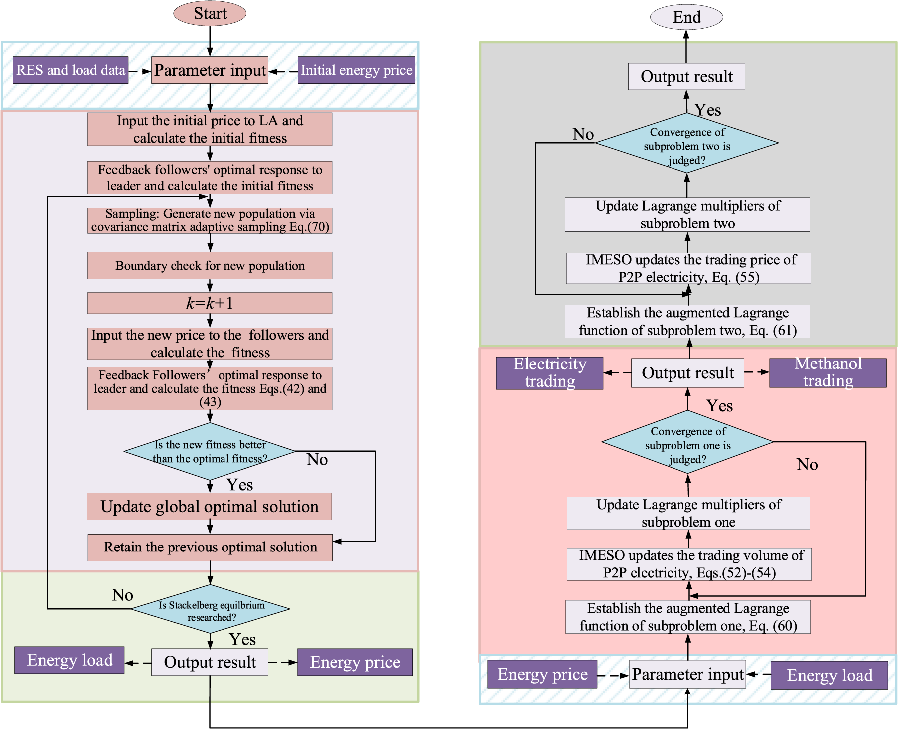
Figure 3: The overall solving process of Stackelberg-Nash game model.

4.1 Solving the Upper-Layer Stackelberg Game

For the upper-layer Stackelberg game model constructed in this paper, the pricing decision of IMESO is essentially a high-dimensional continuous optimization problem with continuous decision variables, with 24-h DR electricity price and 24-h DR heat price forming a 48-dimensional decision variable space. The problem has the characteristics of non-convex objective function, complex constraint coupling and high solution dimension. Traditional algorithms have the defects of premature convergence, insufficient search efficiency in high-dimensional space and poor robustness to non-convex problems. In contrast, CMA-ES realizes dynamic optimization of search step size and search direction by adaptively updating the covariance matrix of the sampling distribution, which can effectively avoid premature convergence, has excellent global optimization performance for high-dimensional nonlinear non-convex problems, and does not depend on gradient information of the objective function, which is highly suitable for solving the upper-layer Stackelberg game problem.

For each group of price strategy [34] individuals generated by CMA-ES iteration, the optimal load response of LA can be obtained through the analytical solution of quadratic programming, and the fitness value of the individual can be calculated by substituting it into IMESO revenue objective function. The specific solving steps are as follows:

Initialization: Set the parameters of CMA-ES, including population size λ, initial search point m, initial step size σ, maximum number of iterations Gmax and convergence threshold ε. In this paper, we adopt the standard optimal configuration of CMA-ES with the following specific parameter settings: Population size: λ is 20; number of selected elite individuals: μ is 10; convergence threshold: ε is 0.001; initial step size: σ is 0.3; Initialize the evolution path Pc and Pσ, as well as the covariance matrix C to the identity matrix.

Sampling and LA optimal response solving: Generate λ groups of candidate price strategy individuals through multivariate normal distribution sampling, as given by

xk∼𝒩(m,σ2C),k=1,2,⋯,λ(70)

Substitute each group of candidate price strategies into the LA optimal response model, solve the optimal load response of LA through Eqs. (40) and (41), verify the satisfaction of load adjustment constraints, and eliminate invalid individuals that do not meet the constraints.

Fitness calculation: Substitute the LA optimal load corresponding to the valid candidate individuals into IMESO objective function Eq. (1), calculate IMESO operating revenue corresponding to each individual, and take the negative value of the revenue as the fitness value for sorting.

CMA-ES iterative update: Select the first μ optimal individuals with the best fitness value, and update the distribution mean m, evolution paths Pc and Pσ, step size σ and covariance matrix C in turn according to the weighted information of the optimal individuals, so as to realize the adaptive optimization of the sampling distribution.

The convergence of the proposed iterative solution algorithm can be further guaranteed as follows. Let zk=[pk,xk] denote the decision vector at the k-th iteration, where pk represents the upper-level decision of IMES and xk represents the lower-level decisions of LAs. The iterative solution process can be written as a fixed-point mapping:

z(k+1)=T(zk)(71)

According to the strict concavity of the objective functions proved in Eqs. (44)–(49), each optimization subproblem has a unique optimal response. Therefore, the mapping T(⋅) is single-valued. In addition, the feasible regions of all participants are closed, bounded and convex, and the objective functions are continuously differentiable. Hence, the best-response mapping is continuous. Since the coupling coefficients among IMES and LAs are bounded by the operational constraints and price limits, there exists a constant ρ∈(0,1) such that

‖T(za)−T(zb)‖≤ρ‖za−zb‖,za,zb∈Ω(72)

where Ω is the joint feasible region of all participants. Therefore, T(⋅) is a contraction mapping on Ω.

According to the Banach fixed-point theorem, the sequence {zk} generated by the proposed iterative algorithm converges to a unique fixed point z∗, namely,

z∗=T(z∗)(73)

At this fixed point, IMES achieves its optimal decision given the Nash equilibrium response of LAs, while each load aggregator obtains its optimal strategy under the decision of IMES. Therefore, the fixed point z∗ is exactly the Stackelberg–Nash equilibrium of the proposed bi-level game. This proves that the proposed iterative algorithm converges to the unique equilibrium point.

Convergence Judgment: The iteration process terminates when the number of iterations reaches the pre-specified maximum value Gmax or the change of the optimal fitness value for consecutive multiple generations is less than the convergence threshold ε, stop the iteration. The optimal individual corresponding to the current optimal fitness value is Stackelberg equilibrium solution, output the optimal DR electricity and heat price, LA optimal load response, and the maximum operating revenue of IMESO [35].

4.2 Solving the Lower-Layer Nash Bargaining Game

The lower-layer alliance optimization involves coupling constraints and distributed decision-making requirements of multiple IMES, and its input parameters are derived from the optimal operation results of a single IMES obtained by the upper-layer CMA-ES solution. Through the decomposition-coordination mechanism, ADMM decomposes the global optimization problem of the alliance into local sub-problems of each IMES, and can achieve global convergence with only a small amount of information interaction between IMES, which effectively protects the data privacy of each subject and adapts to the distributed decision-making characteristics of multi-IMES alliance.

Problem decomposition: Decompose the alliance total revenue maximization problem into local optimization subproblems of N IMES, introduce consistent dual variables and Lagrange multipliers to coordinate the coupling constraints of P2P transaction power between IMES, and split the global objective function into the sum of local objective functions of each IMES.

Local subproblem solving: Under the given dual variables and Lagrange multipliers, each IMES independently solves its own equipment operation strategy and P2P transaction plan with the goal of maximizing its own revenue, updates the local P2P transaction power variables, and sends the updated results to the alliance coordination center.

Global variable update: The alliance coordination center aggregates the local variables of each IMES, updates the global consistent variables of P2P transaction power, and adaptively adjusts the dual variables and Lagrange multipliers according to the consistency deviation of local variables.

Convergence judgment: If the primal residual and dual residual of the iterative process are both less than the set convergence threshold, stop the iteration and output the optimal P2P transaction strategy and the maximum total revenue of the alliance; otherwise, return to step 2 to continue the iteration.

Revenue distribution: Based on the optimal operation results of the alliance, calculate the comprehensive contribution index from the two dimensions of carbon abatement contribution and power contribution, and complete the fair distribution of alliance revenue through Nash bargaining model shown in Eq. (61).

5  Case Study

5.1 Basic Data of the Case

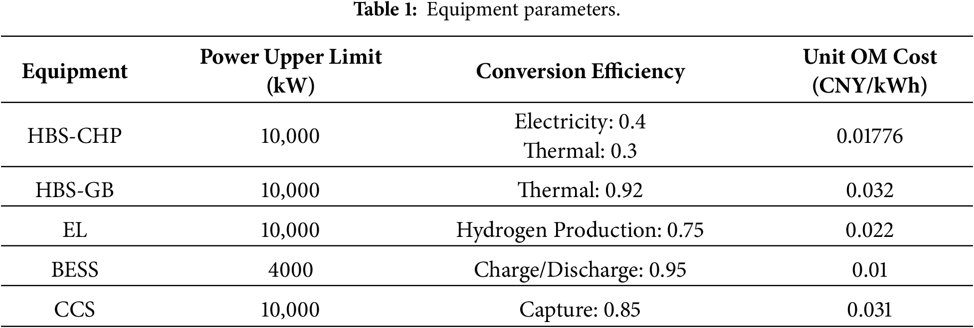
This paper takes three interconnected IMES as the research object, the scheduling cycle is 24 h, and the time step is 1 h. The core equipment parameters are shown in Table 1. ADMM parameters are adopted from [36]. A rigorous theoretical proof of the convergence of ADMM for non-convex optimization problems can be found in reference [37]. The parameter configurations and constraint conditions employed in this paper fully satisfy the sufficient conditions for convergence.

The grid electricity selling price πgrid,sell is 0.30 CNY/kWh. ToU electricity purchasing price πgrid,buy is set as follows: 1.10 CNY/kWh for the periods of 11:00–14:00 and 18:00–22:00; 0.88 CNY/kWh for the periods of 8:00–10:00 and 15:00–17:00; 0.60 CNY/kWh for the periods of 00:00–07:00 and 23:00–24:00. The thermal price has an upper limit of 0.60 CNY/kWh and a lower limit of 0.20 CNY/kWh. The natural gas purchasing price πgas,buy is 3 CNY/m3.

5.2 Result Analysis of the Upper-Layer Model

Figs. 4–6 show the convergence curves of the upper Stackelberg game [38] of IMESO #1 to IMESO #3, respectively, and illustrate the dynamic game of IMESO and LA.

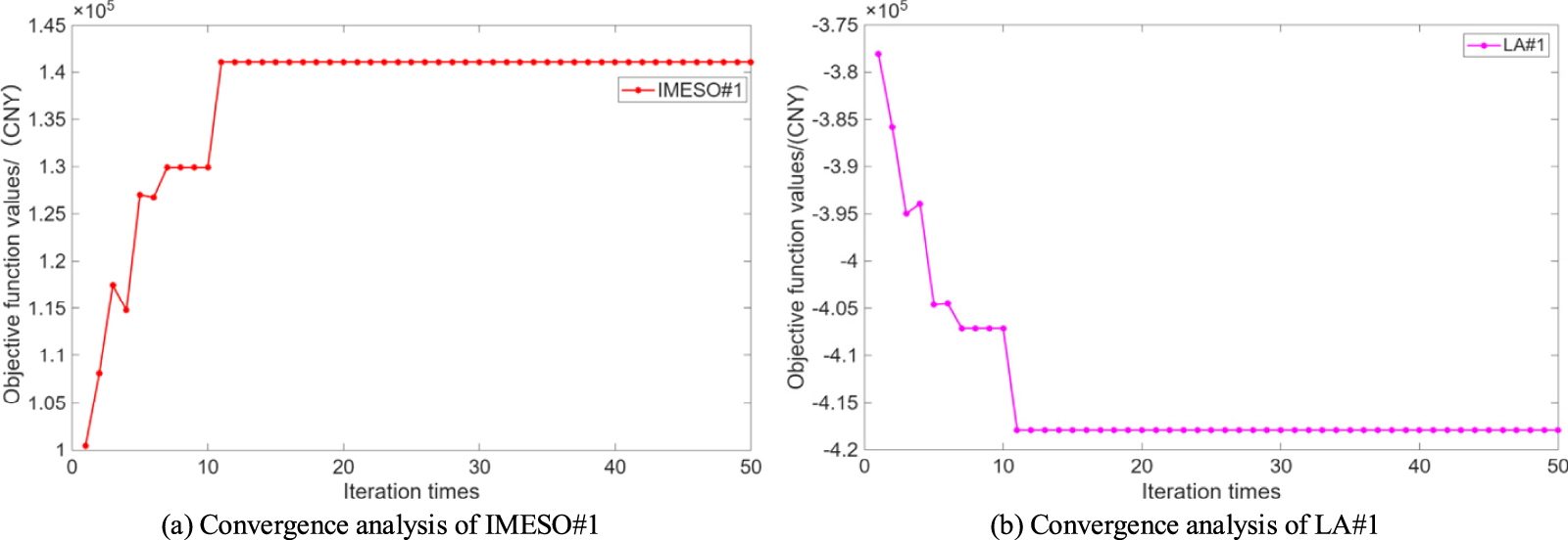
Figure 4: Convergence curves of the upper Stackelberg game of IMES #1.

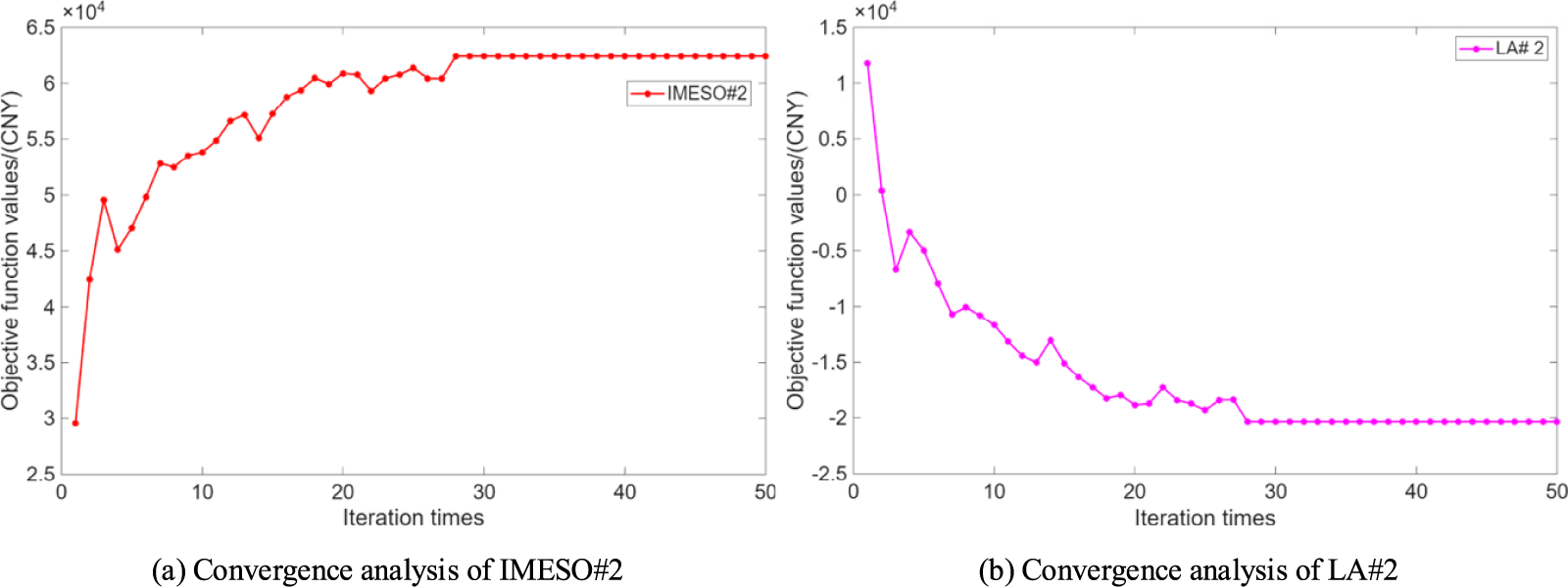
Figure 5: Convergence curves of the upper Stackelberg game of IMES #2.

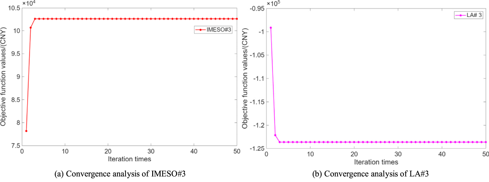
Figure 6: Convergence curves of the upper Stackelberg game of IMES #3.

It can be seen from Fig. 4 that the objective function of IMESO #1 converges after 12 iterations. The objective function of LA #1 converges after 12 iterations.

It can be seen from Fig. 5 that the objective function of IMESO #2 converges after 28 iterations. The objective function of LA #2 converges after 28 iterations.

It can be seen from Fig. 6 that the objective function of IMESO #3 converges after 3 iterations. The objective function of LA #3 converges after 3 iterations.

Fig. 7 shows the electricity price and heat price of each IMES after Stackelberg game.

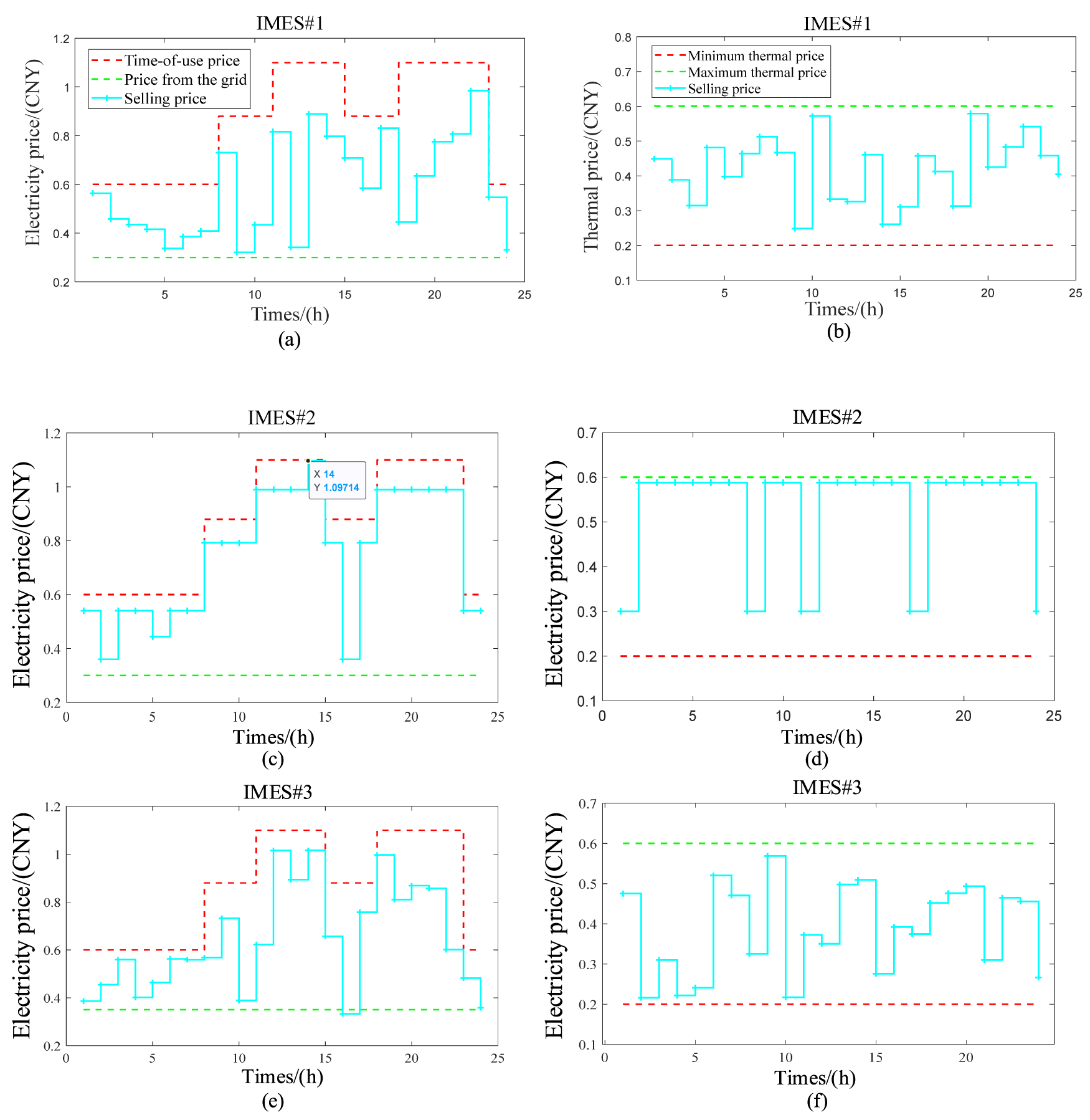
Figure 7: The Stackelberg equilibrium electricity and thermal prices for each IMES. Subfigures (a,c,e) illustrate the intraday electricity price curves for IMES #1, IMES #2, and IMES #3, respectively. Subfigures (b,d,f) depict the corresponding thermal price curves derived from the Stackelberg game.

The electricity pricing strategies of IMES exhibit distinct intraday fluctuation patterns that are highly coupled with the peak-valley characteristics of the power grid’s ToU tariff. The Stackelberg equilibrium achieves joint optimization of electricity and thermal pricing, balancing multiple objectives: ensuring reasonable profit margins for IMES, maintaining price acceptability for end users, and adapting to intraday energy supply-demand fluctuations via ToU dynamic pricing [39]. The resulting strategy establishes a robust trade-off between the economic efficiency and operational rationality of IMES.

Fig. 8 shows the comparison of electrical and thermal loads before and after DR in each IMES.

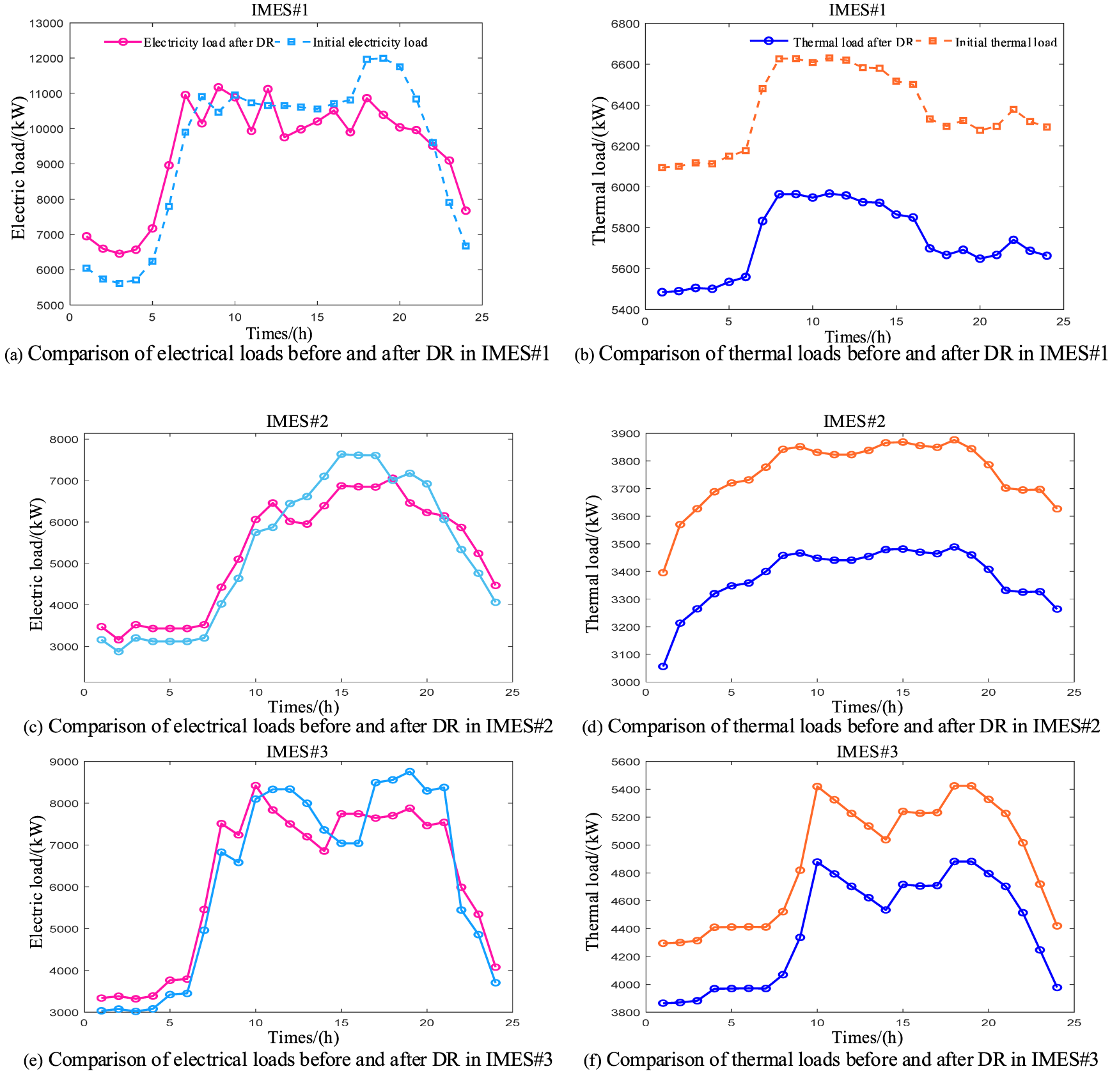
Figure 8: Comparison of electrical and thermal loads before and after DR in each IMES.

It can be seen from Fig. 8 that 10:00–20:00 is the peak period of electricity consumption. The electrical load after DR is significantly lower than the initial electrical load, which successfully achieves peak shaving of electricity consumption and reduces the power supply pressure of IMES during peak hours. 0:00–8:00 is the valley period, where the electrical load after DR is higher than the initial value. This guides users to shift their electricity consumption to low-price periods, fills the load valley, and improves the equipment utilization rate during valley hours. For the thermal load, the peak period is 8:00–18:00, and the valley period is 0:00–6:00.

The results of Fig. 8 verify that the implementation of DR strategy can effectively guide users to adjust their energy consumption behaviors. It not only relieves the peak-valley pressure of energy supply in IMES and improves the operation efficiency of the system [40], but also smooths load fluctuations and enhances the operation stability of the system.

In order to verify the superiority of the proposed algorithm, differential evolution optimization (DEO), particle swarm optimization (PSO) algorithm and genetic algorithm (GA) are compared with CMA-ES, as shown in Fig. 9.

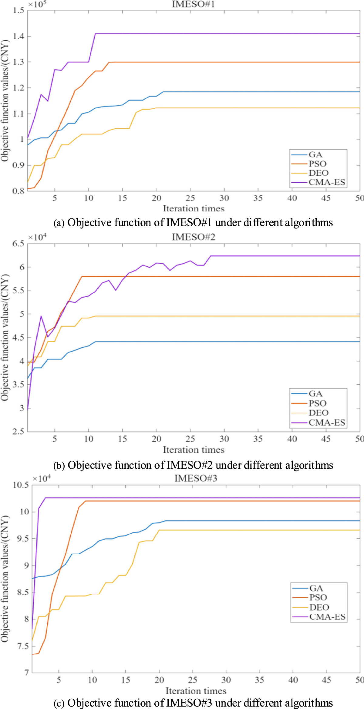
Figure 9: Objective function of IMESO #1–IMESO #3 under different algorithms.

From Fig. 9, in IMESO #1–3, CMA-ES is improved by 11,242 CNY, 4371 CNY and 1154 CNY compared with PSO objective function., respectively.

5.3 Result Analysis of the Lower-Layer Model

The thermal and electrical load operation results of IMES #1–IMES #3 are shown in Fig. 10.

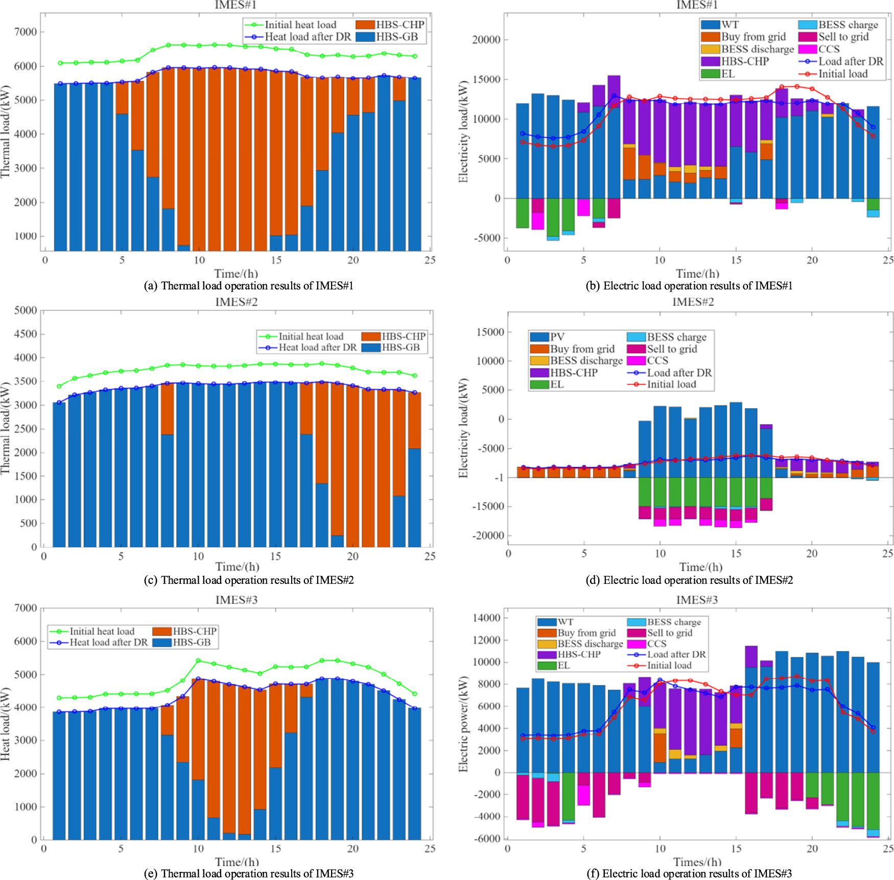
Figure 10: Thermal and electrical load operation results.

From Fig. 10, thermal load after DR exhibits distinct diurnal variation characteristics. The heat load stays low during late night and early morning hours, and rises gradually to its peak between 8:00 and 18:00 in the daytime. The real-time supply-demand balance of thermal power is achieved through the coordinated output of two types of heat sources, namely HBS-CHP and HBS-GB.

The electrical load after DR also presents the typical feature of daytime peak and nighttime trough. Specifically, the load remains at a low level from 0:00 to 6:00 in the early morning, increases rapidly after 7:00, maintains a high level from 10:00 to 20:00, and decreases gradually after 20:00. The supply-demand balance of electric power is realized via the joint operation of HBS-CHP, RES and BESS. Among them, BESS charges during load valley periods and discharges during peak load periods to smooth out load fluctuations, while power purchased from the utility grid serves as supplementary power supply when the power generation is insufficient.

Fig. 11 is the simulation results of natural gas and hydrogen. The diagram clearly shows the output and consumption of hydrogen and natural gas in IMES #1–IMES #3. Negative indicates consumption, and positive indicates output.

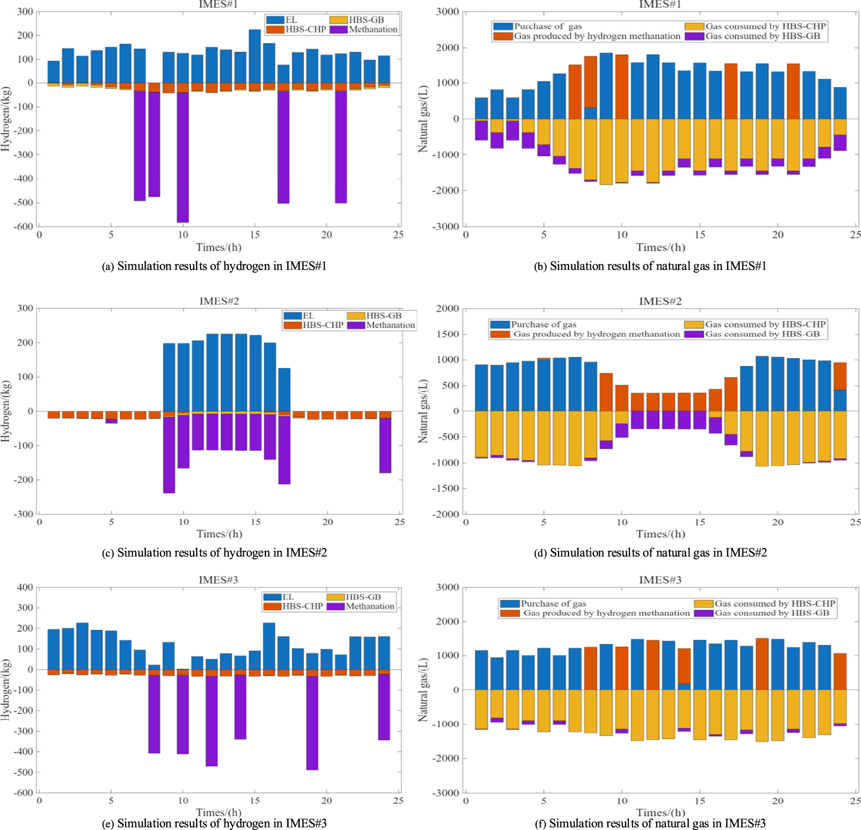
Figure 11: Simulation results of natural gas and hydrogen.

5.4 Impact of Bargaining Power Factors on Revenue Distribution

To further verify the effectiveness of the proposed fairness evaluation framework and the optimal bargaining power factors, we present detailed simulation results of different bargaining scenarios.

Fig. 12 shows the variation of JFI with different values of α. JFI increases rapidly as α decreases from 0 to 0.25, reaches the peak at α=0.25, and then gradually decreases as α further decreases to 0. This trend confirms that overemphasizing either single factor will lead to unfair distribution, while an appropriate balance between the two can achieve the optimal equity. In this paper, α=0.25, β=0.75. Fig. 13 compares the income distribution under different α and β values.

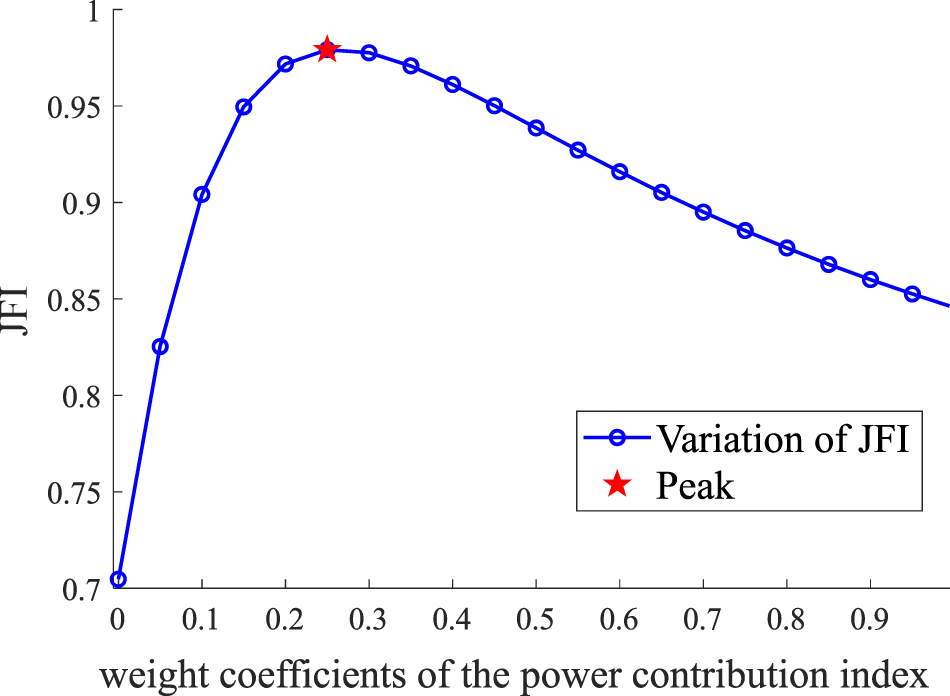
Figure 12: Variation of JFI with different bargaining power factors.

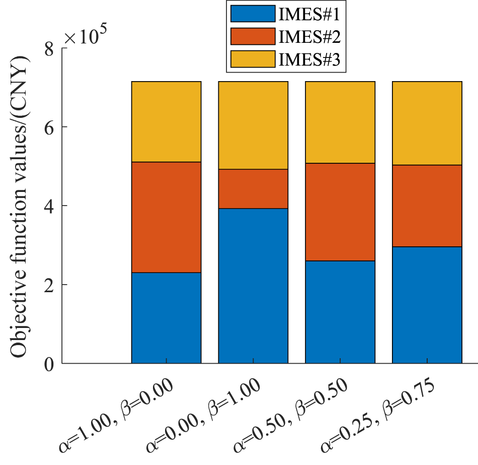
Figure 13: Income distribution under different α and β values.

5.5 Comparative Analysis of Different Game Schemes

Five test scenarios are set up to comprehensively evaluate and analyze the performance of the proposed method.

(1)   Scenario #1: Without considering cooperative game, only consider DR.

(2)   Scenario #2: Without considering DR, the sell price of electricity and thermal is calculated according to the average price of electricity, and only the cooperative game is considered.

(3)   Scenario #3: Consider DR and cooperative game.

(4)   Scenario #4: Consider DR and cooperative game, without CCS.

(5)   Scenario #5: Consider DR and cooperative game, without HBS.

Table 2 compares the effects of the five schemes.

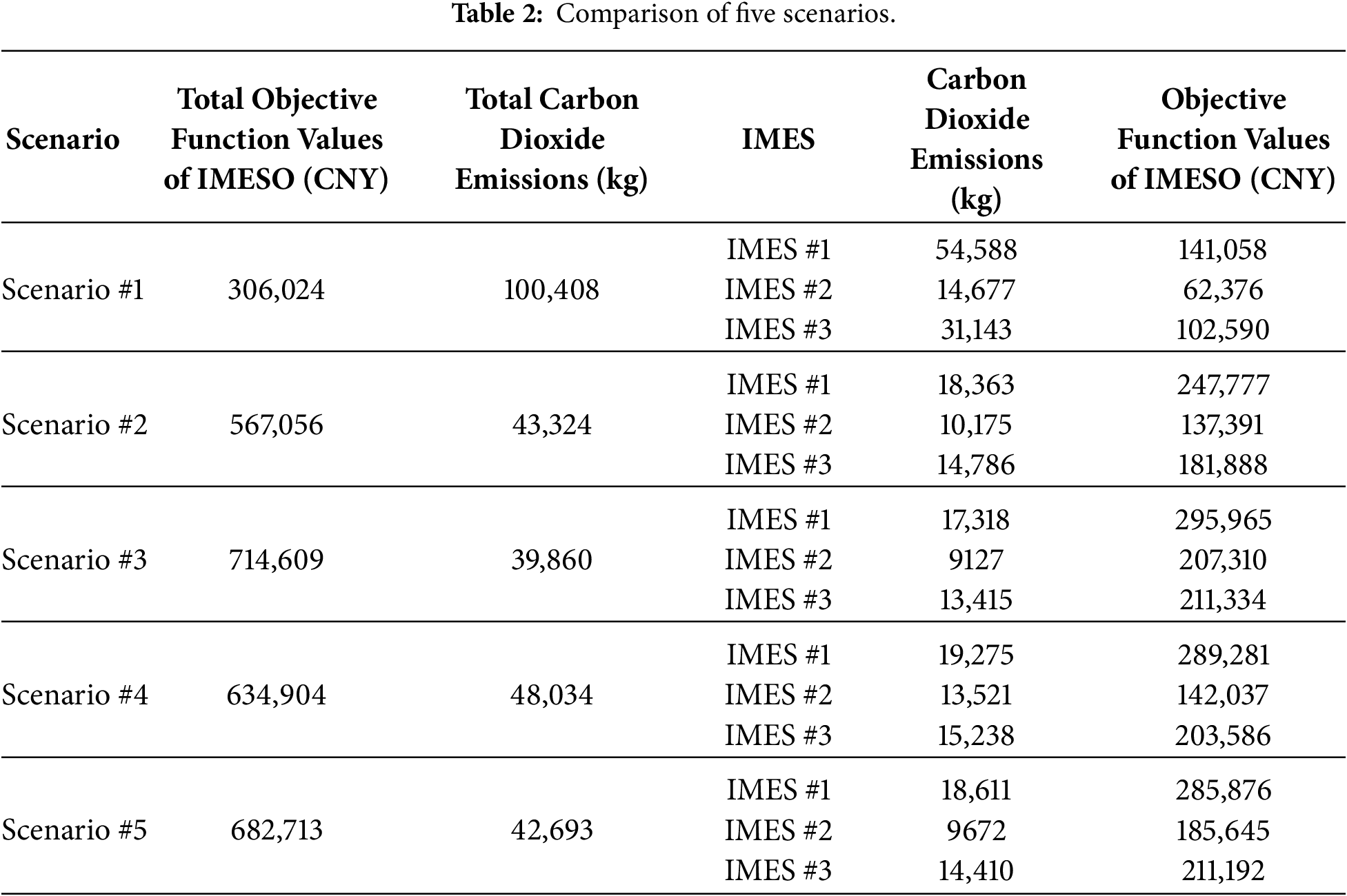
Under Scenario #3, compared with Scenario #1: The constructed model realizes a carbon emission decrease of 37,270 kg for IMES #1, 5550 kg for IMES #2, and 17,728 kg for IMES #3; The revenue of the IMESO objective function is increased by 175,656, 103,688 and 129,241 CNY, respectively. The total carbon emission is reduced by 60,548 kg, and the total IMESO profit is increased by 408,585 CNY. Compared with Scenario #2: The constructed model realizes a carbon emission decrease of 1045 kg for IMES #1, 1048 kg for IMES #2, and 1371 kg for IMES #3; The revenue of the IMESO objective function is increased by 48,188, 69,919 and 29,446 CNY, respectively. The total carbon emission is reduced by 3464 kg, and the total IMESO profit is increased by 147,553 CNY. Compared with Scenario #4 (without CCS): The constructed model realizes a carbon emission decrease of 1957 kg for IMES #1, 4394 kg for IMES #2, and 1823 kg for IMES #3; The revenue of the IMESO objective function is increased by 6684, 65,273 and 7748 CNY, respectively. The total carbon emission is reduced by 8174 kg, and the total IMESO profit is increased by 79,705 CNY. Compared with Scenario #5 (without HBS): The constructed model realizes a carbon emission decrease of 1293 kg for IMES #1, 545 kg for IMES #2, and 995 kg for IMES #3; The revenue of the IMESO objective function is increased by 10,089, 21,665 and 142 CNY, respectively. The total carbon emission is reduced by 2833 kg, and the total IMESO profit is increased by 31,896 CNY.

5.6 Robust Uncertainty Analysis

A significant concern is the treatment of uncertainty arising from RES. The intermittent nature of wind and solar power introduces substantial volatility into the system. Explicitly incorporating this uncertainty into the scheduling model is critical for reliable and optimal operation of IMES.

Box uncertainty sets are adopted to characterize the fluctuation ranges of PV output, load, and wind output. To avoid over-conservative robust solutions, constraints on the maximum number of extreme fluctuation periods are introduced.

The actual PV output fluctuates within ±15% of the predicted value and the actual electrical load fluctuates within ±10% of the predicted value with a maximum of 12 extreme fluctuation periods per day. Generate 50 independent uncertainty scenarios by randomly sampling PV output, electrical load, or wind output uncertainties, covering most extreme operating conditions. Solve LA’s optimal load response and IMESO’s revenue for each sampled scenario, selecting the scenario that minimizes the IMESO’s revenue as the worst-case scenario.

Figs. 14–16 show the uncertainty fluctuation range of IMES #1–IMES #3 load and the worst operation scenario obtained by screening.

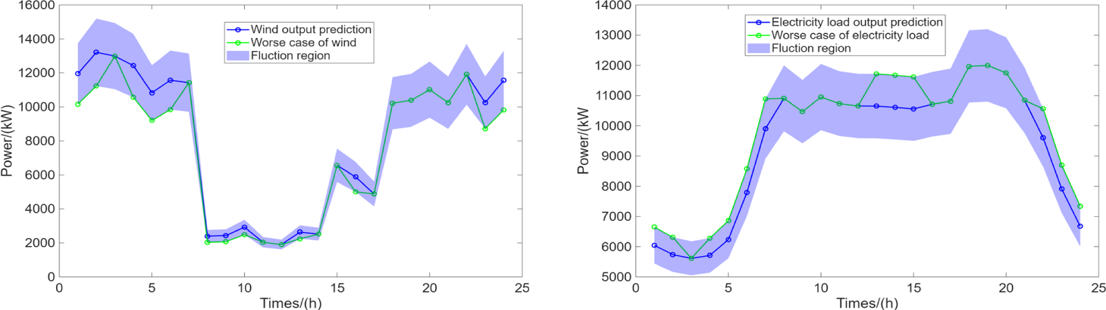
Figure 14: Worst scenario in IMES #1.

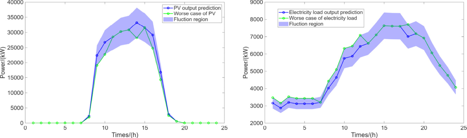
Figure 15: Worst scenario in IMES #2.

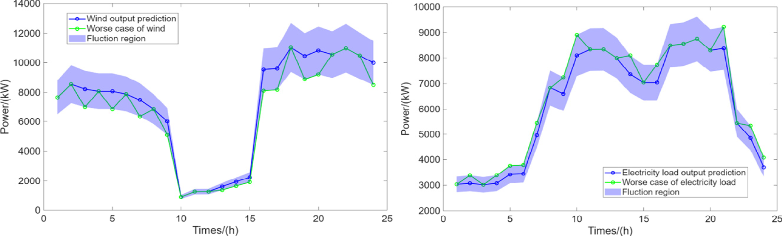
Figure 16: Worst scenario in IMES #3.

From the three cases, several findings are drawn to validate the proposed framework:

Uncertainty coupling is the core risk: The worst-case scenarios consistently coincide with periods of low renewable output and high load demand, rather than isolated extreme fluctuations of a single variable. This confirms that the primary risk to system reliability stems from the coupling of RES intermittency and load volatility, which cannot be addressed by deterministic scheduling alone.

Uncertainty profiles are system-specific: The three IMES exhibit distinct worst-case patterns tailored to their energy mix. Wind-dominated systems face risks during daytime wind troughs, while PV-dominated systems face risks during midday generation peaks. This highlights the necessity of a tailored robust strategy rather than a one-size-fits-all solution.

Complementary risks enable cross-system mitigation: The worst-case periods across the three IMES are complementary (e.g., IMES #2’s midday PV surplus can offset IMES #1’s daytime wind deficit). This provides a clear rationale for the multi-IMES collaborative scheduling proposed in this work, where cross-system reserve sharing can reduce the overall cost of robustness compared to individual system-level risk mitigation.

Table 3 further illustrates the impact of RES uncertainty on IMESO returns.

From Table 3, across all three IMESO, operating benefits under the worst-case scenario are consistently lower than under the normal scenario. This confirms that the coupling of renewable intermittency and load volatility threatens system reliability and also increases operational costs.

Collectively, the identified worst-case scenarios also provide a solid foundation for the subsequent collaborative scheduling analysis, where cross-system reserve sharing is used to mitigate the impact of these uncertainties.

5.7 Carbon Price Sensitivity Analysis

Carbon price is a core policy instrument that governs the trade-off between economic profitability and low-carbon transformation in IMES. Its fluctuations directly affect the operational decisions of IMESO, the utilization intensity of low-carbon technologies (HBS and CCS), and the overall system performance. To quantitatively evaluate the impact of carbon price variations on the proposed scheduling framework, a systematic sensitivity analysis is conducted by varying the carbon penalty coefficient.

The sensitivity analysis results are presented in Fig. 17, which depicts the variations in total system carbon emissions and total IMESO profit as functions of carbon price.

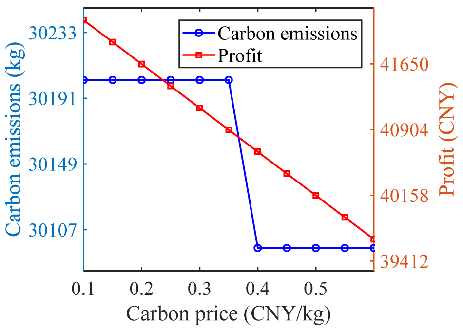
Figure 17: Sensitivity analysis of carbon price.

The above results show that with the increase of carbon price, IMES profit decreases linearly. Under this framework, the fluctuation of carbon emissions is concentrated in 0.35–0.4 CNY/kg.

5.8 Scalability Analysis

This study only verifies the proposed method on three IMES. In theory, the method can be extended to scenarios with 10 or 20 IMES.

The original Nash bargaining product increases exponentially with the number of participants N, and the dimension of P2P transaction matrix rises at the order of O(N2), which brings computational challenges. To address this issue, logarithmic transformation is adopted to convert the multiplicative Nash objective into a linear additive form, effectively eliminating the exponential growth of objective function complexity. Meanwhile, sparsity characteristics of practical energy trading are utilized to simplify the O(N2) transaction matrix, and the alternating direction method of multipliers is introduced for distributed decentralized solution. Such design reduces overall computational burden and maintains stable solution efficiency under multi-agent scenarios.

In this paper, only a small-scale case is conducted for verification. Further research will focus on large-scale scenarios containing more integrated energy systems to further verify the scalability and practical applicability of the proposed strategy.

6  Conclusion

The conclusions of this paper are as follows:

(1)   The bi-level Stackelberg-Nash game collaborative optimization framework constructed in this paper realizes the deep coupling between the master-slave game within a single IMES and the Nash bargaining game among multiple IMES coalitions. By optimizing the electricity and thermal prices after DR, the balance of interests between the supply and demand sides is realized.

(2)   The IMES low-carbon architecture of HBS, EL and CCS built in this paper realizes the full-dimensional collaborative optimization of low-carbon technology, price-based DR and P2P power trading mechanism. The case study results show that compared with the operation mode without cooperative game, the proposed method can reduce the carbon emissions of the system by 60.31%, increase the total revenue by 133.5%, and improve the economic and environmental benefits.

(3)   This paper proposes a comprehensive contribution index based on power contribution index and carbon abatement contribution index, and constructs an income distribution mechanism linked to the actual comprehensive contribution of the participants. It not only guarantees the individual income of the alliance participants, forms an effective positive incentive, but also provides an institutional guarantee for the long-term stable operation of multi-IMES alliance.

(4)   In this paper, a hierarchical solution strategy combining CMA-ES and ADMM is proposed. The adopted CMA-ES algorithm outperforms PSO, with the objective function values of IMESO #1–#3 increased by 11,242 CNY, 4371 CNY and 1154 CNY, respectively. ADMM algorithm realizes the distributed solution of the coalition optimization problem through the decomposition-coordination mechanism.

Acknowledgement: Not applicable.

Funding Statement: This research was funded by National Natural Science Foundation of China (62263014) and Yunnan Province Major Science and Technology Project (202602AF080004).

Author Contributions: Conceptualization, Yang Liu and Bo Yang; methodology, Shuai Zhou; software, Yang Liu and Ning Yang; validation, Yang Liu, Bo Yang, Shuai Zhou and Ning Yang; formal analysis, Bo Yang; investigation, Shuai Zhou; resources, Ning Yang; data curation, Yang Liu; writing original draft preparation, Yang Liu and Shuai Zhou; writing-review and editing, Bo Yang, Ning Yang and Shuai Zhou. All authors reviewed and approved the final version of the manuscript.

Availability of Data and Materials: Not applicable.

Ethics Approval: Not applicable.

Conflicts of Interest: The authors declare no conflicts of interest.

Nomenclature

References

1. Zhou P, Lv Y, Wen W. The low-carbon transition of energy systems: a bibliometric review from an engineering management perspective. Engineering. 2023;29(1):147–58. doi:10.1016/j.eng.2022.11.010. [Google Scholar] [CrossRef]

2. Zou C, Ma F, Pan S, Zhao Q, Fu G, Zhang G, et al. Global energy transition revolution and the connotation and pathway of the green and intelligent energy system. Petrol Explor Dev. 2023;50(3):722–40. doi:10.1016/s1876-3804(23)60423-9. [Google Scholar] [CrossRef]

3. Zhang L, He S, Han L, Yuan Z, Xu L. Multi-energy flow integrated energy system considering economic efficiency targets: capacity allocation and scheduling study. Processes. 2024;12(4):628. doi:10.3390/pr12040628. [Google Scholar] [CrossRef]

4. Liu S, Li X, Xue D. Renewable energy, energy use efficiency and carbon emission intensity: based on the perspective of mediation effect and threshold effect. Mitig Adapt Strateg Glob Change. 2024;29(8):94. doi:10.1007/s11027-024-10193-7. [Google Scholar] [CrossRef]

5. Ye J, Li X, He Y, Ma J, Lv J. Multi-energy coupling characteristic analysis and modeling technology of integrated energy system. In: Proceedings of the 7th IEEE Conference on Energy Internet and Energy System Integration (EI2); 2023 Dec 15–18; Hangzhou, China. p. 939–45. [Google Scholar]

6. Yan J, Zhang J, Zhang L, Deng C, Zhang J, Wang X, et al. Enhanced resilience and efficiency in multi-energy systems via stochastic gradient-driven robust optimization. Prot Control Mod Power Syst. 2026;11(1):141–56. doi:10.23919/pcmp.2024.000412. [Google Scholar] [CrossRef]

7. Yan X, Cao H, Shao C, Wang Z, Jia J. Optimised scheduling for distribution networks, microgrids and demand-side using multi-level game theory. IET Generation Trans Dist. 2025;19(1):e70058. doi:10.1049/gtd2.70058. [Google Scholar] [CrossRef]

8. Jing Y, Liang M, Wang H, Yang Z, Li G, Márquez FPG, et al. Optimal economic and low-carbon scheduling in integrated energy system considering multi-level thermal energy coupling and integrated demand response. Energy Convers Econ. 2025;6(2):83–100. doi:10.1049/enc2.70009. [Google Scholar] [CrossRef]

9. Li J, Ji S, Wang X, Zhang H, Li Y, Qian X, et al. A Stackelberg game-based optimal scheduling model for multi-microgrid systems considering photovoltaic consumption and integrated demand response. Energies. 2024;17(23):6002. doi:10.3390/en17236002. [Google Scholar] [CrossRef]

10. Wang Y, Jin Z, Liang J, Li Z, Dinavahi V, Liang J. Low-carbon optimal scheduling of park-integrated energy system based on bidirectional Stackelberg-Nash game theory. Energy. 2024;305:132342. doi:10.1016/j.energy.2024.132342. [Google Scholar] [CrossRef]

11. Li J, Chen H, Qi Y, Wang Y, Lei J. Collaborative optimization for cross-regional integrated energy systems producing electricity-heat-hydrogen based on generalized Nash bargaining. Energy. 2025;333(2):137444. doi:10.1016/j.energy.2025.137444. [Google Scholar] [CrossRef]

12. Zhao F, Du L, Chu S. Optimized operation strategy for multi-regional integrated energy systems based on a bilevel Stackelberg game framework. Energies. 2025;18(17):4746. doi:10.3390/en18174746. [Google Scholar] [CrossRef]

13. Xue S, Wang Y, Liu Y, Wang Z, Wang Y, Yang D. Bi-level optimization and Stackelberg game in multi-integrated energy systems. J Energy Storage. 2025;111:115356. doi:10.1016/j.est.2025.115356. [Google Scholar] [CrossRef]