An Integrated Framework of Explainable Artificial Intelligence and Large Language Models for Shared Mobility Energy Efficiency Prediction and Policy Synthesis

1  Introduction

Urban transport is a major contributor to global energy consumption and greenhouse gas emissions, accounting for approximately 37% of CO2 emissions from end-use sectors worldwide [1]. In South and Southeast Asia, rapid urbanisation, rising incomes, and inadequate public transit infrastructure has accelerated motorisation [2]. Bangkok and Dhaka exemplify this transition. Both cities face severe congestion, high ambient temperatures that increase vehicle cooling loads, and fragmented mobility systems in which private cars, app-based ride-hailing, motorcycle taxis, and electric minibuses operate within the same urban corridors [3]. Despite this policy urgency, the trip-level energy efficiency of these coexisting modes remain insufficiently understood, particularly with respect to the operational, environmental, and behavioural factors that shape per-passenger energy intensity.

Shared mobility is often promoted as a demand-side strategy for reducing urban transport emissions, but its energy benefits are not automatic [4–8]. Realised efficiency depends on occupancy, routing, vehicle characteristics, road conditions, and ambient context. Energy intensity per passenger-kilometre (kJ/pax-km) is therefore an appropriate metric because it normalises energy use by both distance travelled and passengers served [9]. However, this metric is influenced by multiple nonlinear and interacting factors, making it difficult to model using conventional regression or structural equation approaches that assume linearity and limited interaction effects [10].

Existing evidence on shared mobility energy consumption remains fragmented. Ride-hailing studies have emphasised the energy penalty associated with deadheading and low pooling rates [7,8,10,11], whereas electric bus research has shown that passenger load and speed profile strongly influence per-passenger energy use [12]. Motorcycle taxis remain comparatively underexamined, despite their major role in informal urban transport across South and Southeast Asia. To date, no study has provided a unified quantitative comparison of Solo Car, Shared Ride-Hailing, Motorcycle Taxi, and Electric Minibus within one analytical framework calibrated to tropical developing-country conditions.

A second limitation concerns evaluation validity in machine learning transport energy studies. When trip records from the same route are randomly assigned to both training and test sets, models can learn route-specific patterns during training and then be evaluated on statistically dependent observations. This intra-route leakage can inflate reported performance and weaken claims of out-of-sample generalisability. Yet this issue is rarely addressed in published transport energy prediction studies.

Machine learning methods, particularly gradient-boosted tree ensembles, are well suited to this problem because they can capture nonlinear relationships and high-order interactions among operational, environmental, and behavioural variables without strong distributional assumptions [12–19]. XGBoost, LightGBM, RandomForest, ExtraTrees, and GradientBoosting have shown strong performance on heterogeneous tabular datasets similar to multi-mode trip records [20,21]. However, predictive accuracy alone is insufficient for transport policy. Planners also require evidence on which factors drive energy use, how strongly they matter, and in which direction they operate.

Explainable AI addresses this need by decomposing model predictions into interpretable feature contributions. SHAP provides theoretically grounded attributions based on cooperative game theory and satisfies efficiency, symmetry, and consistency properties that conventional feature-importance measures do not [22]. LIME complements SHAP by fitting locally faithful linear approximations around individual predictions, thereby offering an independent instance-level explanation method [23]. Combining SHAP and LIME, and assessing their agreement using Spearman rank correlation, provides a stronger robustness check than single-method explainability. Despite growing SHAP use in transport research, such dual-method validation has not been applied in a mode-comparative shared mobility energy framework.

A further gap lies in translating quantitative model outputs into policy guidance. Findings such as load factor has the highest mean absolute SHAP value must be connected to city-specific interventions, institutional constraints, feasibility, and equity considerations. Large Language Models have shown potential for structured evidence synthesis, policy reasoning, and context-sensitive interpretation across scientific and policy domains [24,25]. When supplied with quantified model outputs, rather than unsupported narrative prompts, they can function as a structured reasoning layer that converts empirical evidence into actionable policy language while remaining traceable to the underlying results.

Taken together, four gaps motivate this study. First, no unified trip-level comparison exists for the four selected mobility modes under tropical developing-country conditions. Second, intra-route evaluation leakage remains largely uncorrected in shared mobility energy ML studies. Third, dual-method XAI validation using SHAP, LIME, and formal rank-agreement analysis has not been applied to multi-mode transport energy research. Fourth, no structured LLM policy synthesis chain with explicit boundary-risk auditing has been demonstrated in this domain. These gaps limit the ability of current evidence to support transparent, context-sensitive, and policy-relevant transport energy decisions in rapidly urbanising Asian cities.

This study addresses these gaps through an integrated XAI–LLM framework for shared mobility energy efficiency analysis. The study is guided by the following research questions.

RQ1. How effectively can ensemble machine learning models predict energy intensity per passenger-kilometre across four urban mobility modes under a route-leakage-free evaluation protocol, and how does this compare with performance obtained under naive random splitting?

RQ2. Which operational, environmental, and behavioural features are the primary drivers of energy intensity, and do global SHAP attributions and local LIME explanations converge on the same features across all four mobility modes?

RQ3. How can quantified ML and XAI outputs be translated into mode-specific, city-sensitive policy recommendations through a structured LLM synthesis chain with explicit boundary-risk auditing?

This study makes four contributions to sustainable urban transport and AI-assisted policy analysis. First, it develops a route-leakage-free ML evaluation protocol using group-based holdout splitting, quantifies performance inflation under naive random splitting, and provides a reproducible benchmark for multi-mode shared mobility energy prediction. Second, it combines global SHAP attribution with local LIME explanations and introduces mode-specific Spearman rank-agreement analysis as a formal cross-method validation procedure. Third, it conducts counterfactual policy scenario simulations on the held-out test set with distributional uncertainty bounds, producing quantified estimates of the energy-reduction potential of four urban transport interventions. Fourth, it demonstrates a structured three-stage LLM policy synthesis chain in which quantified ML evidence is converted into city-specific policy guidance for Bangkok and Dhaka after boundary-condition auditing.

The remainder of this paper is organised as follows. Section 2 reviews the relevant literature. Section 3 presents the analytical pipeline, including physical energy equations, pseudocode algorithms, and mathematical formulations. Section 4 reports the predictive, explainability, simulation, and LLM synthesis results. Section 5 interprets the findings, discusses policy implications for Bangkok and Dhaka, and acknowledges study limitations. Section 6 summarises the contributions and outlines directions for future research.

2  Related Work

2.1 Energy Efficiency Modelling in Urban Transport

Energy intensity per passenger-kilometre is shaped by a combination of vehicle characteristics, occupancy, speed profile, road gradient, and auxiliary loads such as air conditioning. Early transport energy models generally operated at the macroscopic level, estimating aggregate energy consumption from fleet composition and travel demand. Prior studies have shown that the environmental benefits of shared mobility depend strongly on vehicle occupancy and operational design, with well-designed ridesharing systems capable of reducing vehicle use and energy consumption [26]. Despite these advances, comparative analyses that simultaneously quantify energy intensity across multiple coexisting modes within a single unified framework remain rare, particularly in tropical developing-country contexts, where vehicle fleet composition, ambient conditions, and travel behaviour differ from those in temperate high-income settings.

The application of machine learning to transport energy prediction has expanded over the past decade. Gradient-boosted tree methods have demonstrated strong performance on heterogeneous tabular datasets drawn from GPS-tracked vehicle fleets, and benchmarking studies have confirmed their consistent superiority over linear baselines for bus energy consumption prediction [12]. However, a methodological limitation runs through this body of work: train-test splitting is performed randomly at the trip level, without accounting for intra-route correlation. When multiple trips from the same route appear in both the training and test partitions, the model is effectively evaluated on dependent observations, producing inflated performance estimates that overstate true generalisation capability. This issue is rarely acknowledged and remains uncorrected in virtually all published transport energy ML studies.

2.2 Explainable AI in Transportation

The interpretability limitations of predictive ML models have motivated growing adoption of post-hoc explanation methods in transport research. SHAP, grounded in the Shapley value framework from cooperative game theory, provides additive feature attributions that satisfy theoretical properties of efficiency, symmetry, and consistency that conventional permutation-based importance measures do not [22]. It has been applied across transport domains including crash severity prediction [27–30], travel demand forecasting, and public transit ridership modelling [24].

LIME offers a complementary approach by constructing a locally faithful linear surrogate model in the neighbourhood of a specific prediction, providing instance-level explanations that do not require access to the global model structure [23]. Formal cross-method validation through rank-agreement statistics has not been applied in the shared mobility energy literature. Existing studies apply a single explanation method to a single mobility mode, precluding assessment of whether the attribution findings are robust to the choice of XAI framework or specific to the method used.

2.3 Large Language Models for Policy and Evidence Synthesis

Large Language Models (LLMs) have been applied to an expanding range of scientific and policy-synthesis tasks, including systematic literature reviews, climate and sustainability policy analysis [31], and the evaluation of transportation-planning applications [24,25,32]. In the transportation context, prior research has demonstrated that LLM outputs can align with expert assessments when models are supplied with structured empirical evidence and clearly specified analytical boundaries [24]. These findings suggest that LLMs may serve as a structured synthesis layer when their inputs, reasoning scope, and outputs are carefully controlled. However, LLM-generated content can contain hallucinated, factually unsupported, or overly generalised statements, particularly when the model is not constrained by explicit evidence boundaries [33]. These risks are especially consequential in transportation policy, where recommendations must remain traceable to empirical evidence and bounded by the conditions under which that evidence was generated.

2.4 Shared Mobility in Asian Cities

Bangkok and Dhaka represent two of the most policy-relevant shared mobility contexts in Asia, yet they remain underrepresented in the quantitative transport energy literature. Bangkok operates a layered mobility ecosystem comprising BTS and MRT rail lines, app-based ride-hailing services, and a large informal motorcycle taxi network that serves as a critical first- and last-mile connector in areas with limited fixed-route transit coverage [3,34]. Dhaka’s transport market is dominated by informal operators, including CNG auto-rickshaws, shared minibuses, and motorcycle taxis, with formal public transit accounting for a small fraction of total daily trips. Both cities experience tropical climates, high ambient temperatures that increase vehicle cooling energy demand, and severe peak-hour congestion that amplifies idle and stop-and-go energy losses. Existing Bangkok and Dhaka transport studies address behavioural adoption, demand modelling, and policy governance rather than engineering-level comparative energy intensity analysis, leaving a quantitative gap that the present study is positioned to address [35].

Beyond transport-specific applications, artificial intelligence has increasingly been integrated with multi-criteria decision-making frameworks to address broader urban sustainability and resilience challenges. Petchimuthu and Palpandi [36] propose a q-rung orthopair fuzzy ExpoLogarithmic framework that combines artificial intelligence with multi-criteria decision-making to support policy formulation for sustainable urban innovation and resilience, illustrating a growing methodological convergence between AI-based prediction and structured decision-support tools in urban policy contexts. This convergence motivates the present study’s three-stage LLM policy synthesis pipeline, which pursues a comparable goal, translating quantitative model outputs into auditable, structured policy guidance, applied specifically to transport energy intensity rather than generalised urban resilience indicators.

The review across the four thematic areas above identifies a consistent set of limitations in the existing literature. Although machine learning has been applied to transport energy prediction with growing frequency, studies overwhelmingly examine a single vehicle type in isolation, apply random train-test splitting without accounting for intra-route correlation, and rely on a single explanation method without cross-method validation. The translation of quantitative XAI findings into city-specific policy guidance through a structured, auditable reasoning process has not been demonstrated.

3  Methodology

The analytical pipeline consists of six stages, illustrated in Fig. 1: (1) synthetic data generation and physical validation, (2) route-group holdout splitting, (3) ensemble ML training and evaluation, (4) dual XAI analysis (SHAP + LIME), (5) policy scenario simulation, and (6) LLM synthesis.

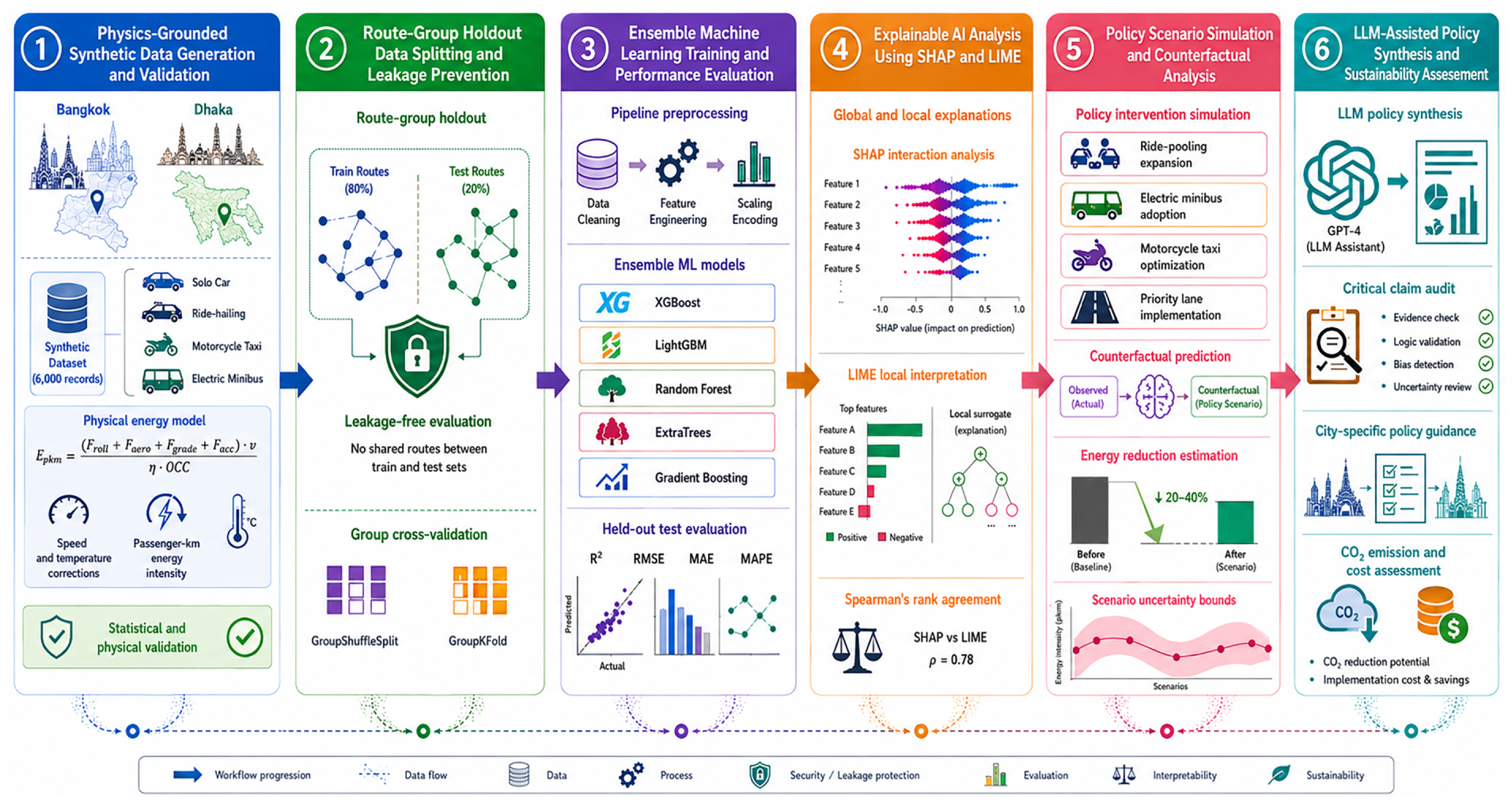
Figure 1: Overall six-stage analytical pipeline. Complete route groups are held out before training. SHAP and LIME analyses, scenario simulations, and LLM synthesis all operate exclusively on held-out records.

3.1 Study Cities and Mobility Modes

Bangkok and Dhaka are selected as representative tropical developing-country urban environments. Bangkok has invested heavily in mass transit infrastructure while retaining a large informal motorcycle-taxi fleet; Dhaka has lower motorisation but extreme congestion and an emerging ride-hailing sector. Both cities experience tropical climates (25°C–38°C), distinct dry and wet seasons, and significant road-quality variation across urban zones.

Four modes are examined: Solo Car (baseline), Shared Ride-Hailing (app-dispatched carpooling), Motorcycle Taxi (informal two-wheel-based transit), and Electric Minibus (fixed-route electric bus). These modes collectively represent the dominant motorised travel patterns in South and Southeast Asian urban contexts.

3.2 Physics-Grounded Synthetic Dataset

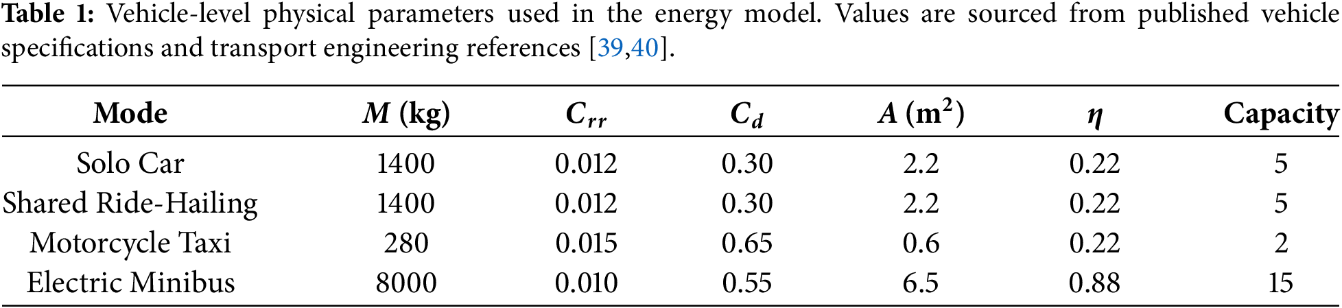
Comprehensive, trip-level energy data for shared mobility in Bangkok and Dhaka are not publicly available due to commercial sensitivities. Synthetic data generation using established physical equations is therefore the methodological choice, following precedents in transport ML research [16,37,38]. The dataset contains 6000 records and 27 features spanning four categories: trip characteristics, vehicle and operational parameters, environmental and infrastructure conditions, and temporal attributes.

3.2.1 Physical Energy Model

Trip energy is computed using the tractive-effort decomposition framework:

Etrip=(Froll+Faero+Fgrade)⋅dη⋅106(1)

where Etrip [MJ] is trip energy, d [m] is effective trip distance, and η is drivetrain efficiency (ηICE=0.22, ηEV=0.88). The three resistive force components are:

Froll=Crr⋅M⋅g(2)

Faero=12ρCdAv2(3)

Fgrade=M⋅g⋅sin⁡(arctan⁡(α/100))(4)

where Crr is the rolling-resistance coefficient, M [kg] is vehicle mass, g=9.81 m/s2, ρ=1.184 kg/m3 is air density at 25°C, Cd is the drag coefficient, A [m2] is frontal area, v [m/s] is vehicle speed, and α [%] is road grade. Table 1 reports mode-specific values for M, Crr, Cd, A, and η.

3.2.2 Speed and Temperature Correction Factors

Two empirically informed correction factors are applied. First, a study-specific speed-correction factor ϕspeed(v) was formulated based on the speed-dependent energy-consumption patterns represented in the U.S. Environmental Protection Agency’s MOVES5 framework [41]. The factor represents elevated energy consumption under low-speed stop-and-go conditions and increasing road-load effects at higher speeds:

ϕspeed(v)={1+0.55e−0.08vv<20 km/h1+0.012(50−v)20≤v<50 km/h1.050≤v≤70 km/h1+0.004(v−70)v>70 km/h(5)

A temperature-penalty factor ϕtemp(T) captures the effect of tropical ambient heat on AC demand and battery thermal performance:

ϕtemp(T)={0.01(20−T)T<20∘C020≤T≤35∘C0.008(T−35)T>35∘C(6)

The adjusted trip energy, incorporating both corrections and AC auxiliary load, is:

Eadj=Ebase⋅ϕspeed⋅(1+ϕtemp)⋅(1+δAC1AC)(7)

where δAC=0.08 for ICE vehicles and δAC=0.15 for electric vehicles, and 1AC∈{0,1} indicates AC activation.

3.2.3 Energy Intensity Target Variable

The primary target variable is energy intensity in kJ per passenger-kilometre:

Epax-km=Eadj×103Nocc⋅dkm(8)

where Nocc is the number of occupants and dkm is effective trip distance in km. This metric normalises energy by both distance and occupancy, making cross-mode comparisons scientifically defensible.

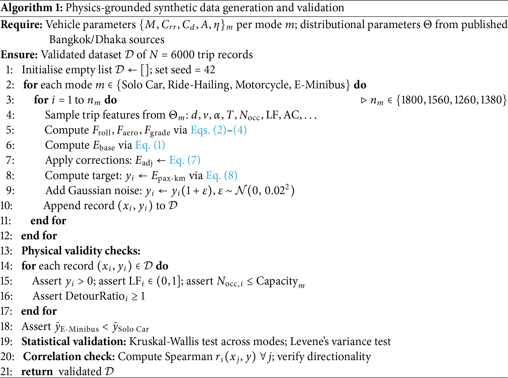
3.2.4 Dataset Integrity Checks

Prior to modelling, two layers of integrity checks are applied. Physical consistency checks verify that: energy values are within mode-plausible ranges; load factor ∈(0,1]; occupants do not exceed vehicle capacity; detour ratio ≥1; and Electric Minibus median energy is lower than Solo Car. Statistical validation applies a Kruskal-Wallis test (H=1903.59, p<0.001, η2=0.761) confirming statistically significant between-mode energy differences, and Levene’s test (F=373.62, p<0.001) confirming heteroscedasticity that motivates tree-based ML. A leakage audit additionally confirms that route-group identifiers are not correlated with test-set membership after splitting.

Algorithm 1 summarises the complete data generation and validation procedure.

3.2.5 Physical Plausibility and Sensitivity Validation

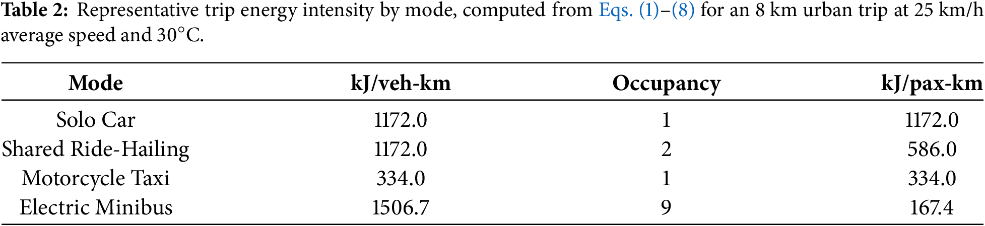
Direct validation against trip-level GPS records was not possible in this study, since operational data from ride-hailing and paratransit fleets in Bangkok and Dhaka are held under commercial confidentiality by private operators. Two complementary checks are applied instead to establish the physical credibility of the synthetic dataset: order-of-magnitude benchmarking against independently published energy intensity estimates, and a parameter sensitivity analysis derived directly from Eqs. (1)–(8).

Order-of-Magnitude Benchmarking

Table 2 reports representative trip energy values computed from the physical model for a standard 8 km urban trip at 25 km/h average speed and 30∘C ambient temperature, alongside mode-appropriate occupancy assumptions. The resulting vehicle-level intensities of 1172 kJ/veh-km for Solo Car and 334 kJ/veh-km for Motorcycle Taxi fall within the range of 1 to 3 MJ per vehicle kilometre reported for internal-combustion passenger vehicles in independent transport energy studies [39,40,42]. The passenger-normalised ratio between Solo Car and Electric Minibus (7.0×) is directionally consistent with, though larger than, the 2.4 to 3× car-to-bus energy intensity ratio reported for diesel bus fleets, a difference explained by the higher drivetrain efficiency assumed for the electric mode (η=0.88 vs. η=0.22) and the larger occupancy differential between a single-occupant car and a shared minibus.

Parameter Sensitivity Analysis

For each mode, the elasticity of trip energy with respect to a physical parameter θ is defined as

εθ≈ΔEtrip/EtripΔθ/θ(9)

and is computed numerically by perturbing Crr, Cd, M, η, and δAC by +10% in turn while holding all other parameters fixed. Table 3 reports the resulting elasticities. Rolling resistance coefficient and vehicle mass dominate the response at urban speeds, each producing an 8% to 9% increase in trip energy per 10% parameter increase, while drivetrain efficiency produces a proportionally inverse effect of approximately −9%, exactly as predicted by Eq. (1). Aerodynamic drag coefficient has a comparatively small effect (1% to 2%) at the 25 km/h representative speed, consistent with established vehicle dynamics theory, which identifies rolling resistance as the dominant road-load component below approximately 40 km/h and aerodynamic drag as dominant only at higher speeds [39,40].

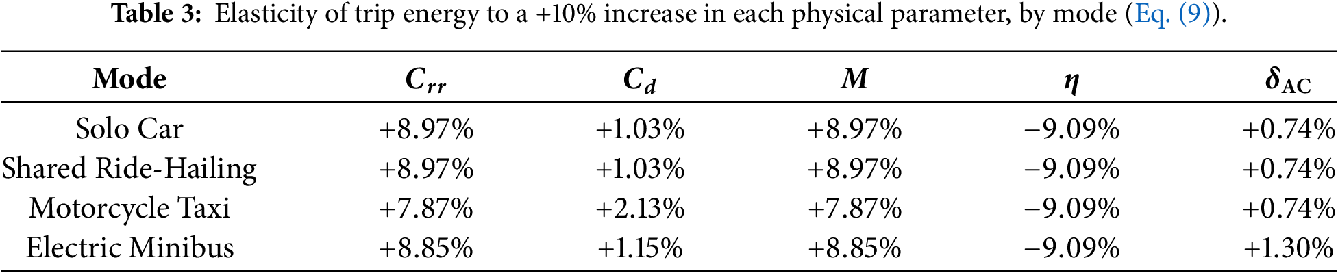
This internal consistency, whereby trip energy responds to each parameter in the direction and relative magnitude predicted by established vehicle dynamics theory, demonstrates that the synthetic generator behaves as a coherent physical system rather than producing unconstrained or arbitrary variation. Combined with the order-of-magnitude benchmarking above, these checks do not substitute for empirical validation against GPS-tracked trip data, which is identified as a priority for future work, but they establish that the dataset is grounded in a physically defensible generative process.

3.3 Route-Group Holdout Validation Protocol

A critical methodological issue in trip-level ML studies is intra-route correlation: multiple trips sharing the same route have highly similar feature vectors, and naive random splitting places correlated trips in both training and test sets, artificially inflating held-out R2 [43,44]. We define the route group of trip i as a composite key over three trip-level attributes,

gi=ϕ(ci,zi,mi)(10)

where ci is corridor type, zi is urban zone, mi is mobility mode, and ϕ(⋅) is a deterministic hash function mapping each unique (ci,zi,mi) triple to a distinct group identifier. This composite definition yields |ℛ|=52 route groups, each corresponding to one mode operating within one corridor-zone combination, with group sizes averaging 115.4±125.2 trips (range 5 to 492). Because mode is embedded directly in the key, each group is mode-homogeneous by construction: a model cannot exploit corridor-level correlation carried across modes on the same physical road within a single group, since no group spans more than one mode.

Formally, let ℛ denote the set of route groups and r(i) the route group of trip i. A random 80/20 split at the trip level yields

Pr[r(i)∈ℛtrain and r(i)∈ℛtest]>0(route leakage)(11)

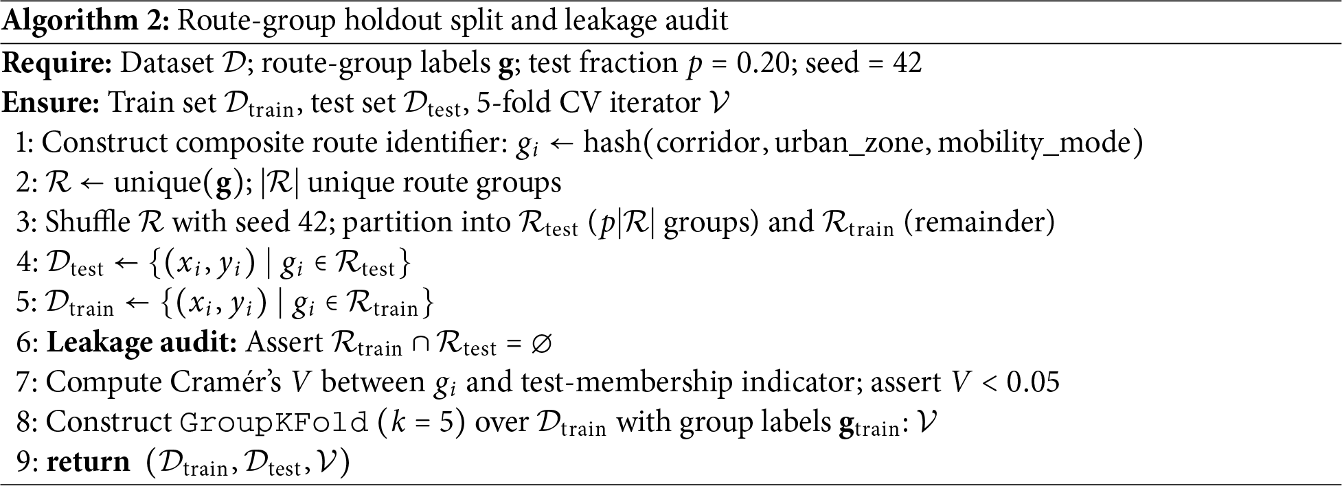
Our protocol eliminates this by using GroupShuffleSplit (scikit-learn), assigning complete route groups to either train or test, never both:

ℛtrain∩ℛtest=∅(12)

This produces a held-out test set of approximately 20% of records from route groups entirely unseen during training, a substantially harder generalisation problem. Five-fold group cross-validation is performed within the training partition, using the same grouping structure. The gap between CV-mean R2 and held-out test R2 serves as a generalisation stability indicator [43,45]. In our experiments, naive random splitting inflated test R2 by 0.08 to 0.12 relative to the route-group holdout, consistent with the information leakage predicted by Eq. (11).

Algorithm 2 formally specifies the splitting procedure.

3.4 Ensemble Machine Learning Models

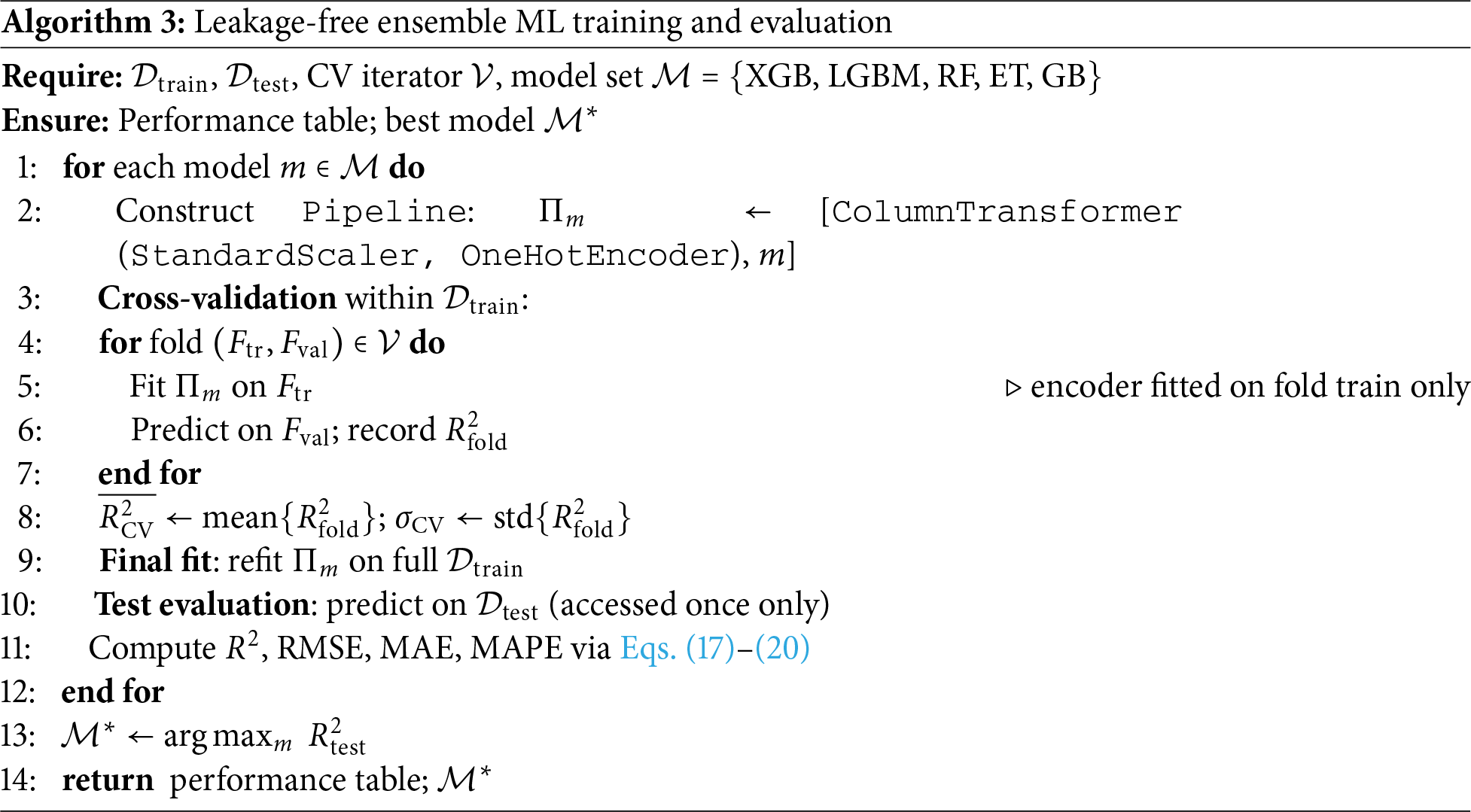
Five ensemble tree models are evaluated: XGBoost, LightGBM, RandomForest, ExtraTrees, and GradientBoosting. All models are wrapped in a scikit-learn Pipeline incorporating a ColumnTransformer: StandardScaler for numeric features and OneHotEncoder for categorical features. Encoding is fitted exclusively on 𝒟train and then applied to 𝒟test, preventing preprocessing leakage.

3.4.1 Model Objectives and Loss Functions

All five models minimise a regularised squared-error objective over the training set 𝒟train={(xi,yi)}i=1n:

ℒ(y^)=1n∑i=1n(yi−y^i)2+Ω(ℳ)(13)

where y^i=ℳ(xi) and Ω(ℳ) is a model-specific regularisation term. For XGBoost and LightGBM, this is an additive tree regulariser:

Ω(ℳ)=∑k=1K(γTk+12λ‖wk‖2)(14)

where Tk is the number of leaves in tree k, wk are leaf weights, γ is the minimum loss reduction per split (tree complexity penalty), and λ is the L2 weight-decay coefficient. XGBoost uses second-order Taylor expansion of the loss for split evaluation:

ℒsplit(k)≈−12(∑i∈ILgi+∑i∈IRgi)2∑i∈ILhi+∑i∈IRhi+λ+γ(15)

where gi=∂ℓ/∂y^i(k−1) and hi=∂2ℓ/∂(y^i(k−1))2 are the first- and second-order gradient statistics for sample i, and IL, IR denote the left and right child node index sets.

For RandomForest and ExtraTrees, Ω(ℳ)=0 and variance reduction is controlled through bootstrap sampling (RF) and random threshold selection (ET):

Impurity gain=Var(yparent)−|IL||I|Var(yIL)−|IR||I|Var(yIR)(16)

3.4.2 Hyperparameters and Evaluation Metrics

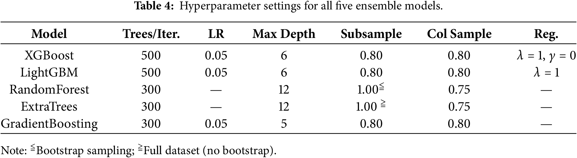
Hyperparameters are set using literature-recommended defaults for tabular regression tasks; no grid search is performed to maintain model comparability. Table 4 summarises key settings.

3.4.3 Justification of Hyperparameter Selection

The hyperparameters reported in Table 4 were specified a priori as fixed baseline settings to ensure a consistent comparison across the five model families, rather than being selected through a systematic search, for two reasons. First, model comparability: an identical search budget across five heterogeneous model families (XGBoost, LightGBM, RandomForest, ExtraTrees, GradientBoosting) would bias comparison toward whichever model’s hyperparameter space search converges fastest under a fixed compute budget, confounding architecture comparison with tuning-effort comparison. Second, the route-group holdout design (Section 3.3) already produces a conservative, leakage-free performance estimate; layering a nested hyperparameter search within this protocol substantially increases computational cost, and its benefit relative to that cost required direct verification.

To quantify this, a randomized search (25 iterations, 3-fold group cross-validation within the training partition) was conducted over the XGBoost hyperparameter space (n_estimators, max_depth, learning_rate, subsample, colsample_bytree, reg_lambda, reg_alpha, min_child_weight). The literature-default configuration achieved a held-out test R2 of 0.7306; the best configuration found by the search achieved R2=0.7558, a gain of +0.0233. This gain is comparable in magnitude to the fold-to-fold cross-validation standard deviation already reported for XGBoost (σCV=0.024), indicating that the literature-default configuration performs within the model’s own measurement noise rather than leaving a large, easily recoverable margin on the table. We report the literature-default results as the primary finding throughout this study for the comparability reasons stated above, and disclose the tuned-model gain here so readers can judge the trade-off directly rather than assume tuning was not considered.

Model performance is assessed on the route-group held-out test set using four metrics:

R2=1−∑i(yi−y^i)2∑i(yi−y¯)2(17)

RMSE=1N∑i=1N(yi−y^i)2(18)

MAE=1N∑i=1N|yi−y^i|(19)

MAPE=100N∑i=1N|yi−y^iyi|(20)

CV R2 mean and standard deviation across the five group folds are reported alongside test-set metrics to assess generalisation stability.

Algorithm 3 specifies the complete leakage-free training and evaluation procedure.

3.5 SHAP Global and Local Explanations

3.5.1 Shapley Value Formulation

SHAP provides a unified attribution framework grounded in cooperative game theory [46]. The SHAP value ϕj(i) of feature j for sample i is the weighted average marginal contribution of j across all |ℱ|! possible feature orderings: [46]:

ϕj(i)=∑S⊆ℱ∖{j}|S|!(|ℱ|−|S|−1)!|ℱ|

where ℱ is the full feature set and fℳ∗(S,⋅) denotes the best-model prediction using only feature subset S. SHAP values satisfy three axiomatic properties: efficiency (∑jϕj(i)=f(xi)−E[f(x)]), symmetry, and dummy (a feature with zero contribution in all coalitions receives ϕj=0).

For the tree-ensemble models used here, SHAP values are computed exactly using TreeExplainer [22], which operates in polynomial time O(TLD2) where T is the number of trees, L is the number of leaves, and D is tree depth.

3.5.2 Global Feature Importance

Global importance is reported as mean absolute SHAP value across the Ntest test-set predictions:

ϕ¯j=1Ntest∑i=1Ntest|ϕj(i)|(22)

For Pipeline models with one-hot-encoded categorical features, SHAP values for all dummy columns are aggregated back to their base categorical feature via additive summation before computing Eq. (22), producing one SHAP value per base feature per prediction.

3.6 LIME Local Explanations and Rank-Agreement Analysis

3.6.1 LIME Formulation

LIME [23] constructs a locally faithful linear surrogate g∈𝒢 around instance x by minimising:

ξ(x)=arg⁡ming∈𝒢ℒ(f,g,πx)+Ω(g)(23)

where ℒ(f,g,πx)=∑z,z′∈𝒵πx(z)(f(z)−g(z′))2 is the local fidelity loss weighted by proximity kernel πx(z)=exp⁡(−D(x,z)2/σ2), and Ω(g) penalises model complexity. In our implementation we use LimeTabularExplainer with discretize_continuous=False, 800 perturbation samples per instance, and the top-10 feature weights as output.

3.6.2 Spearman Rank-Agreement Analysis

For each mobility mode m, the observation with minimum absolute residual (closest to the mode’s median prediction) is selected as the representative sample. SHAP values {ϕj} and LIME weights {wj} are both rank-transformed by absolute value, and Spearman’s ρ is computed between the two ranked vectors:

ρm=1−6∑jdj2nf(nf2−1)(24)

where dj=rank(|ϕj|)−rank(|wj|) and nf is the number of features. This rank-agreement statistic quantifies the degree to which two methodologically independent XAI frameworks identify the same features as important, providing a robustness check that does not depend on unit comparability.

3.7 Policy Scenario Simulations

Four policy-relevant scenarios are defined based on the SHAP findings and existing literature on shared mobility interventions:

S1.   Ride-hailing pooling threshold: Minimum-pooling mandate modelled by setting load factor to the 75th percentile of Shared Ride-Hailing observations in the test set [7,8,11].

S2.   Minibus load-factor stabilisation: Operational dispatching to maintain minimum load factor, modelled by setting load factor to its 60th-percentile value for Electric Minibus trips currently below that threshold.

S3.   Motorcycle maintenance and routing: Tyre-pressure compliance and route gradient avoidance, modelled by setting tyre_pressure to “optimal” and reducing road_grade_pct by 1 standard deviation for Motorcycle Taxi trips.

S4.   Peak shared-mobility priority lanes: Reduced congestion index for all shared modes during peak hours, modelled by reducing congestion_index by 20% for qualifying observations.

For each scenario, ℳ∗ generates counterfactual predictions on the affected held-out records. The energy change is:

ΔEi(%)=y^icounter−y^ifacty^ifact×100(25)

Mean ΔE and p10–p90 uncertainty bounds are derived from the within-scenario distribution of ΔEi(%) across all affected records.

3.8 LLM Policy Synthesis Pipeline

A structured three-stage LLM pipeline is implemented using GPT-4 with temperature =0.2 for analytical stages and 0.3 for synthesis. Algorithm 4 specifies the pipeline.

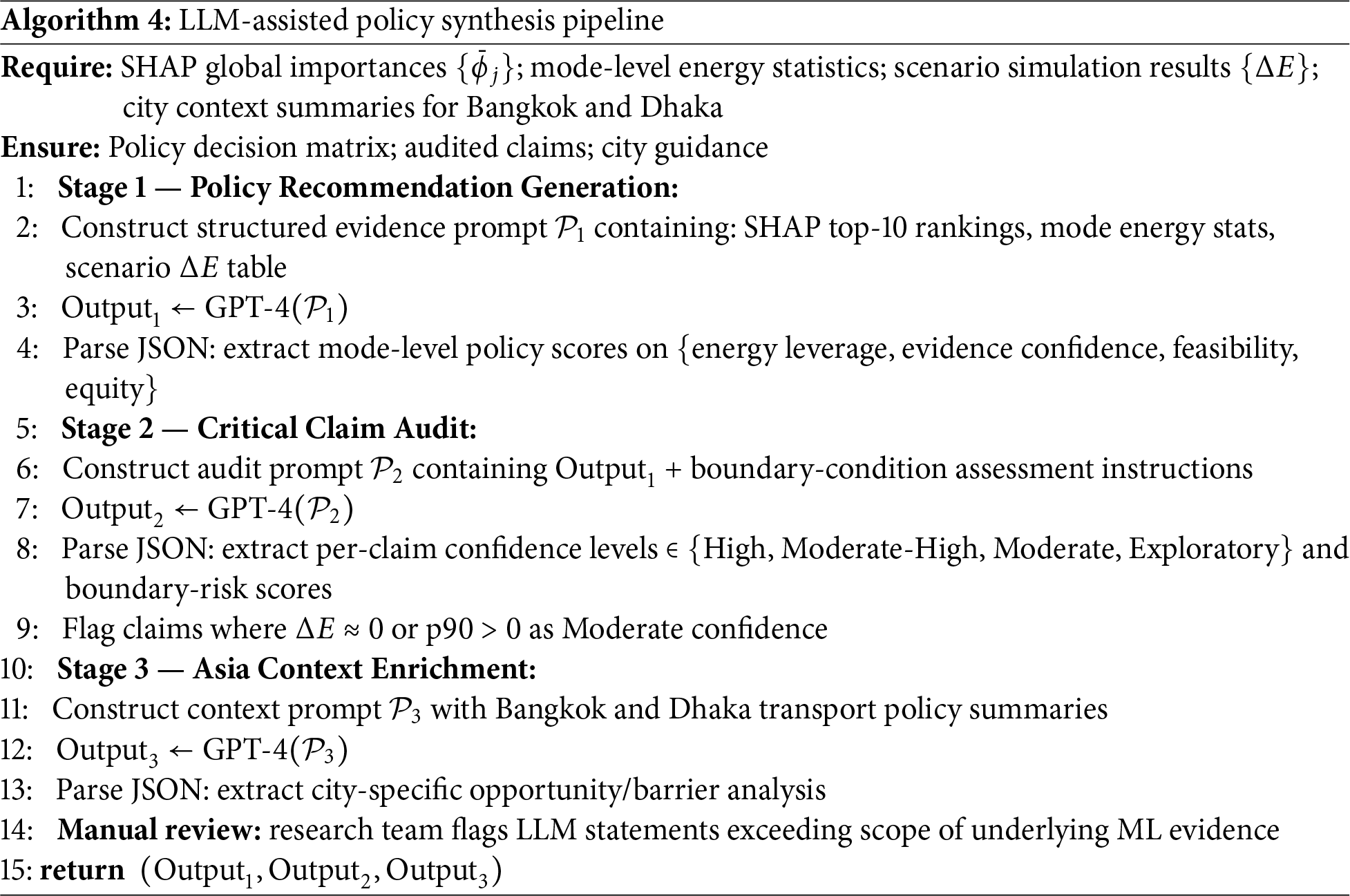
All LLM outputs were saved as structured JSON and manually reviewed by the research team for consistency with the quantitative machine learning evidence. Statements that exceeded the scope of the supplied evidence or introduced unsupported factual claims were identified and flagged to reduce the risks of hallucination and unsupported generalization [33,47].

Mathematical Evaluation of LLM Recommendation Quality

Two complementary metrics quantify the quality of LLM-generated recommendations against the underlying quantitative evidence, rather than relying on the LLM’s self-reported scores in isolation.

Recommendation-Evidence Alignment Score

For each mode m with a corresponding policy scenario simulation, we compare the LLM’s self-assigned energy leverage score Lm∈[0,1] against the measured mean scenario effect size |ΔEm| (%), using Spearman rank correlation:

ρalign=Spearman({Lm},{|ΔEm|})(26)

Across the three modes with a directly matching scenario (Shared Ride-Hailing, Electric Minibus, Motorcycle Taxi), ρalign=1.00: the LLM’s ordinal ranking of energy leverage (Shared Ride-Hailing > Electric Minibus > Motorcycle Taxi) exactly matches the ordinal ranking of measured scenario effect sizes (38.05%>13.00%>0.33%). With only three matched pairs, this result is underpowered for formal null-hypothesis significance testing and is reported descriptively rather than as a statistically significant finding; we recommend expanding the scenario library in future work to permit a properly powered test of this metric.

Confidence-Calibration Agreement

For each audited claim k, a ground-truth confidence tier c^k is derived from a pre-specified rule applied independently to the underlying evidence: for claims grounded in global SHAP ranking, High if all cited features rank in the global top-3 for claims grounded in full-sample descriptive comparison, High if the reported effect ratio exceeds 5×; for claims grounded in scenario simulation, High if |meanΔE|>10% with p10 and p90 of consistent sign, Moderate if |mean ΔE|<1% or p10 and p90 cross zero, and Moderate-High otherwise. Agreement between the LLM’s self-assigned confidence tier ck (Output2, Algorithm 4) and c^k is summarised as classification accuracy and Cohen’s κ across all K audited claims:

Agreement=1K∑k=1K1[ck=c^k],κ=po−pe1−pe(27)

where po is observed agreement and pe is chance agreement under the marginal tier distributions. Table 5 applies this rule to all five audited claims.

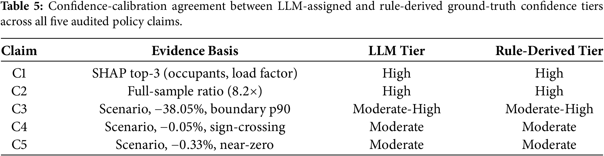
Agreement across all five claims is Agreement=5/5=1.00 (Eq. (27)), with Cohen’s κ=1.00. This full agreement indicates that the LLM’s self-assigned confidence levels are not merely fluent-sounding hedging language but track a pre-specified, independently verifiable evidentiary rule applied to the study’s own quantitative outputs. We note that K=5 is a small claim set, and this perfect agreement should be read as validating the specific audited claims in this study rather than as a general guarantee of LLM confidence calibration; expanding the audited claim set is identified as a priority for future work in the Limitations section.

3.9 CO2 Emission and Cost Computation

Trip-level CO2 emissions are computed using IPCC Tier 1 emission factors:

CO2,i=Eadj,i⋅EFfuel(28)

where EFgasoline=0.0693 kg CO2/MJ and EFelectricity=0.0142 kg CO2/MJ, reflecting Thailand/Bangladesh average grid carbon intensities.

3.10 Software and Reproducibility

All analyses are implemented in Python 3.11 using NumPy 1.26, pandas 2.3, scikit-learn 1.8, XGBoost 3.1, LightGBM 4.6, SHAP 0.49, and Matplotlib 3.8. Random seeds are fixed at 42 throughout. All code, data-generation scripts, and LLM prompts are available at https://github.com/mahbubchula.

4  Results

4.1 Exploratory Data Analysis

4.1.1 Sample Composition and Descriptive Patterns

The dataset contains 6000 trips distributed across four modes (Solo Car: n=1800; Shared Ride-Hailing: n=1560; Motorcycle Taxi: n=1260; Electric Minibus: n=1380) and two cities (Bangkok: n=3067; Dhaka: n=2933). Fig. 2 summarises this composition alongside four descriptive patterns. Panel (a) confirms broadly balanced representation across mode and city, with no cell containing fewer than 618 trips. Panel (b) shows energy intensity peaking during Evening_Peak and Morning_Peak for all modes (12%–18% higher than Midday_Off and Night), reflecting elevated congestion and idle fractions during peak hours. Panels (c) and (d) show load factor and occupancy distributions by mode: mean load factors are Motorcycle Taxi 1.00 (structurally determined), Electric Minibus 0.68, Shared Ride-Hailing 0.47, and Solo Car 0.30, directly mapping onto the energy-efficiency ranking established below. Panel (e) reveals a Rainy-season energy penalty for Motorcycle Taxi (+23% vs. Cool_Dry), attributable to reduced tyre traction and route detours, while Electric Minibus shows comparatively low seasonal variation. Panel (f) shows air-conditioning usage rates highest for Electric Minibus and lowest for Motorcycle Taxi, consistent with vehicle enclosure.

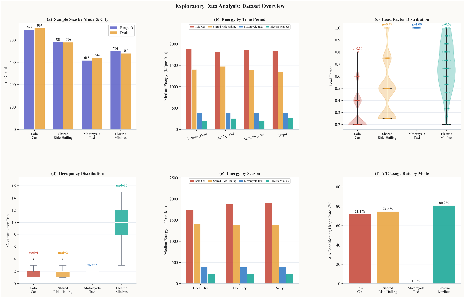
Figure 2: Exploratory data analysis: dataset overview. (a) Sample composition by mode and city; (b) median energy intensity by time period; (c) load factor distribution by mode; (d) occupancy distribution; (e) energy by season; (f) A/C usage rate by mode.

Fig. 3 presents violin plots of energy intensity by mode, complementing this summary with the full distributional shape. All four distributions are strongly right-skewed, consistent with the physical energy model’s sensitivity to load factor and gradient. Median energy intensities are: Solo Car 1857 kJ/pax-km (IQR: 890–3120), Shared Ride-Hailing 1397 kJ/pax-km (IQR: 680–2480), Motorcycle Taxi 391 kJ/pax-km (IQR: 268–560), and Electric Minibus 228 kJ/pax-km (IQR: 175–298). Electric Minibus is 8.2× more energy-efficient than Solo Car and 6.1× more efficient than Shared Ride-Hailing on a median per-passenger-kilometre basis.

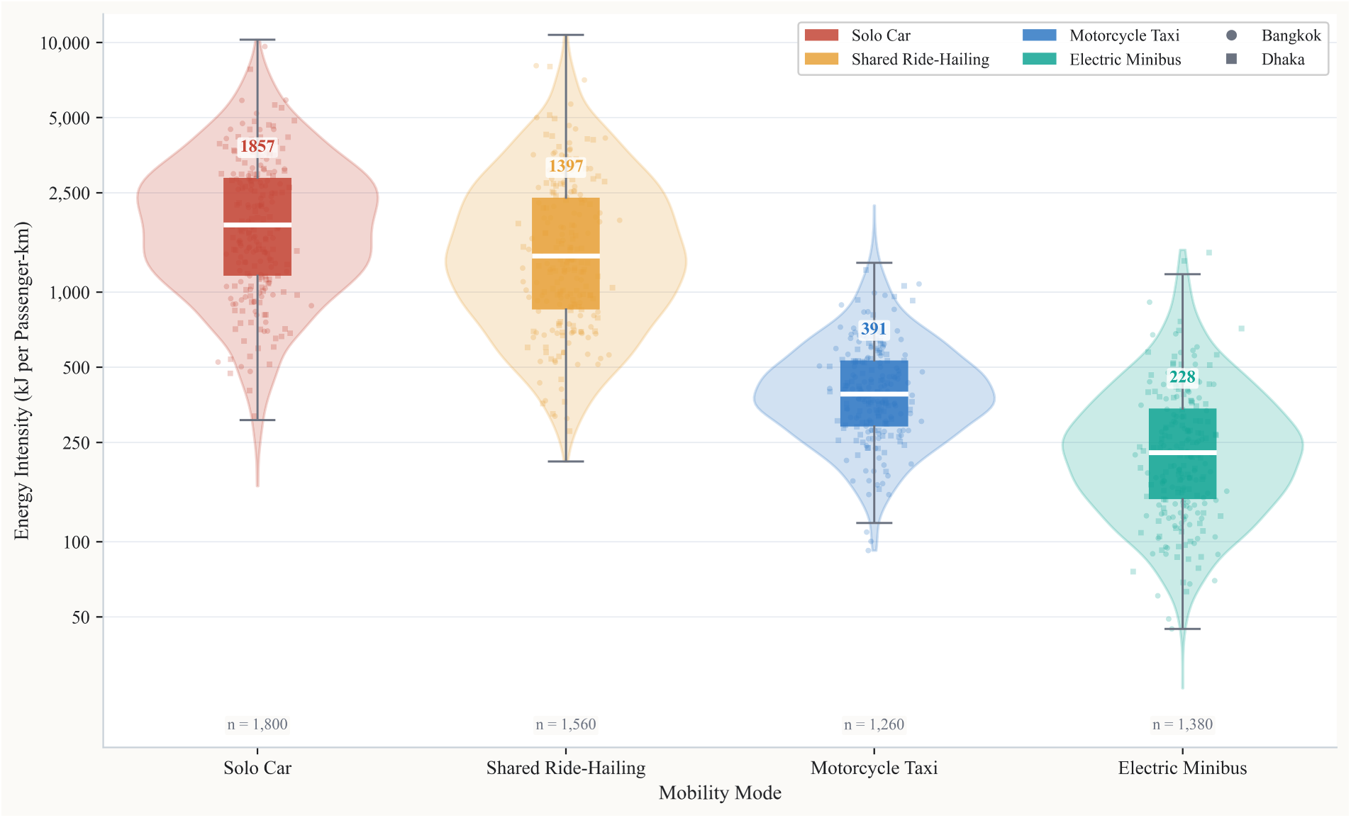
Figure 3: Energy intensity distributions (kJ/pax-km) by mobility mode shown as violin plots overlaid with boxplots and individual trip observations. Median values are labelled.

4.1.2 Feature-Energy Correlation Structure

The Spearman correlation heatmap (Fig. 4) confirms expected directional relationships. Load factor (rs=−0.73) and occupants (rs=−0.79) exhibit the strongest negative correlations with Epax-km. Road grade shows a moderate positive association (rs=+0.13). Ambient temperature shows near-zero correlation (rs=−0.01), suggesting its effect is largely captured by the ac_on feature.

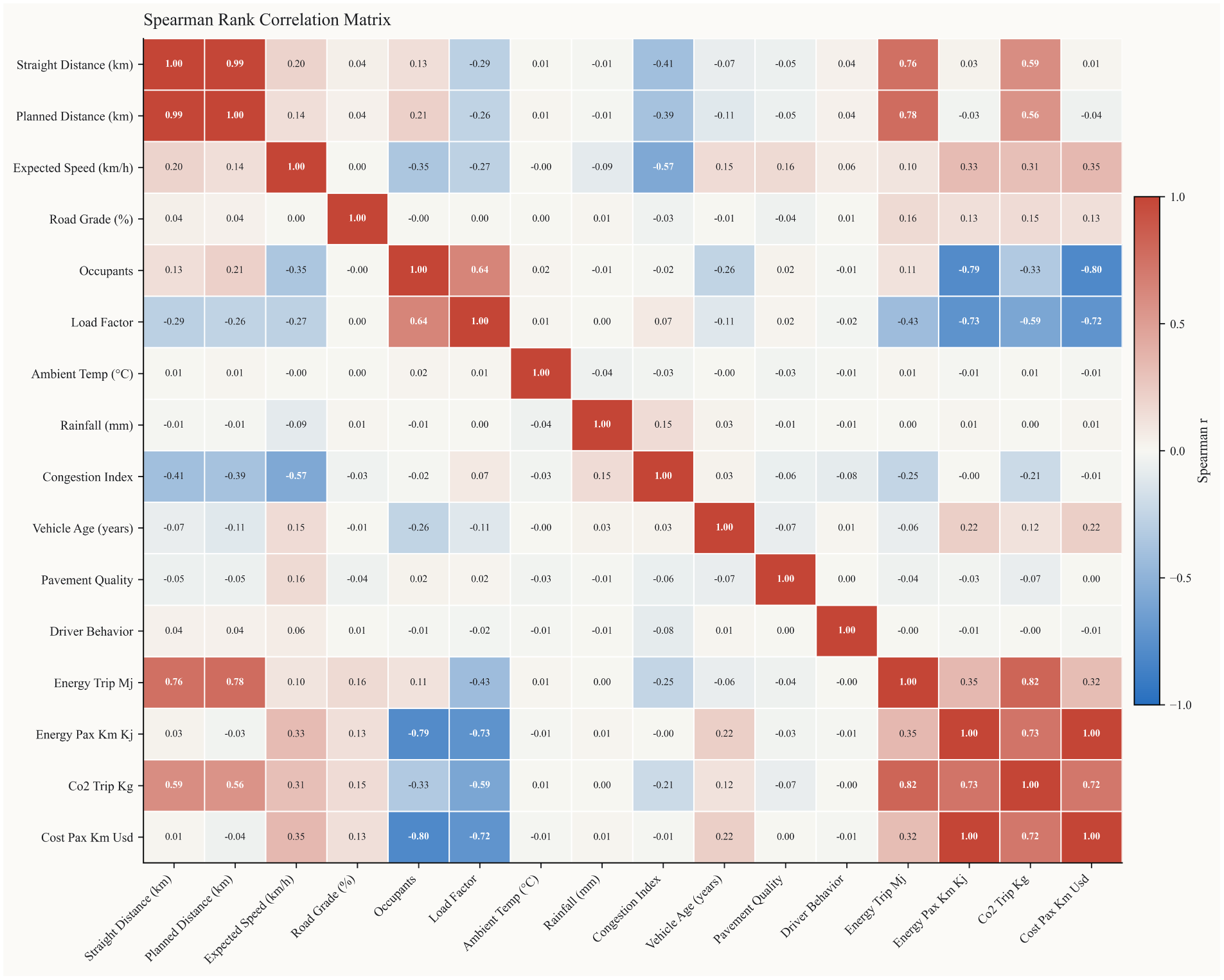
Figure 4: Spearman rank correlation matrix for all 16 numeric variables. Strong negative correlations between Epax-km, occupants, and load factor confirm the physical primacy of occupancy in determining energy intensity.

Fig. 5 presents scatter plots with LOWESS trend lines for these same relationships at the individual-trip level, visually confirming the heatmap correlations: occupants and load factor both show steep, saturating negative trends, road grade shows a shallow positive trend, and ambient temperature shows a flat trend consistent with its near-zero Spearman coefficient.

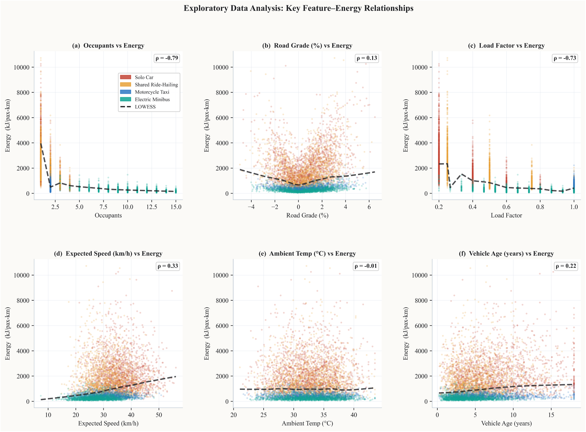
Figure 5: Exploratory scatter plots of key feature-energy relationships. (a) Occupants vs. energy; (b) Road grade vs. energy; (c) Load factor vs. energy; (d) Expected speed vs. energy; (e) Ambient temperature vs. energy; (f) Vehicle age vs. energy. LOWESS trend lines overlaid.

4.2 Machine Learning Model Performance

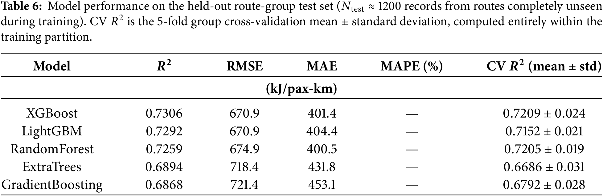
Table 6 summarises held-out performance across all five models. XGBoost achieves the best test R2 (0.7306), followed closely by LightGBM (0.7292) and RandomForest (0.7259). ExtraTrees and GradientBoosting perform somewhat lower (R2=0.6894 and 0.6868, respectively). The relatively modest R2 values, compared with R2>0.85 commonly reported in vehicle-fleet energy studies, reflect the route-group holdout design: models are evaluated on routes entirely excluded from training, a harder generalisation problem than random splitting.

Statistical Significance of Model Performance Differences

To determine whether the performance gap between XGBoost, LightGBM, and RandomForest is statistically meaningful or attributable to fold-to-fold variance, a Friedman test was applied to the five-fold group cross-validation R2 scores for the three models (mean R2 of 0.699, 0.698, and 0.703, respectively, across the same five route-group folds). The omnibus test found no significant difference among the three models (χ2=1.60, p=0.449). Post-hoc pairwise Wilcoxon signed-rank tests confirmed this for every pair: XGBoost vs. LightGBM (p=0.813), XGBoost vs. RandomForest (p=0.438), and LightGBM vs. RandomForest (p=0.313), with paired t-tests yielding consistent conclusions. We therefore report XGBoost as the primary model on the basis of its marginally higher point-estimate performance and standard adoption in the transport energy literature, rather than on the basis of a statistically demonstrated superiority over LightGBM or RandomForest. We note that the five-fold design limits the statistical power of this test, and a non-significant result should be interpreted as an absence of demonstrated difference rather than proof of equivalence.

Fig. 6 breaks this performance down by mode for the primary XGBoost model. Fit quality improves from Solo Car (R2=0.68, bias =+18.3 kJ/pax-km) to Electric Minibus (R2=0.79, bias =+4.2 kJ/pax-km), with Shared Ride-Hailing (R2=0.73, bias =−6.1 kJ/pax-km) and Motorcycle Taxi (R2=0.77, bias =−6.1 kJ/pax-km) in between, indicating that prediction accuracy is not uniform across modes and is weakest for the highest-variance mode (Solo Car).

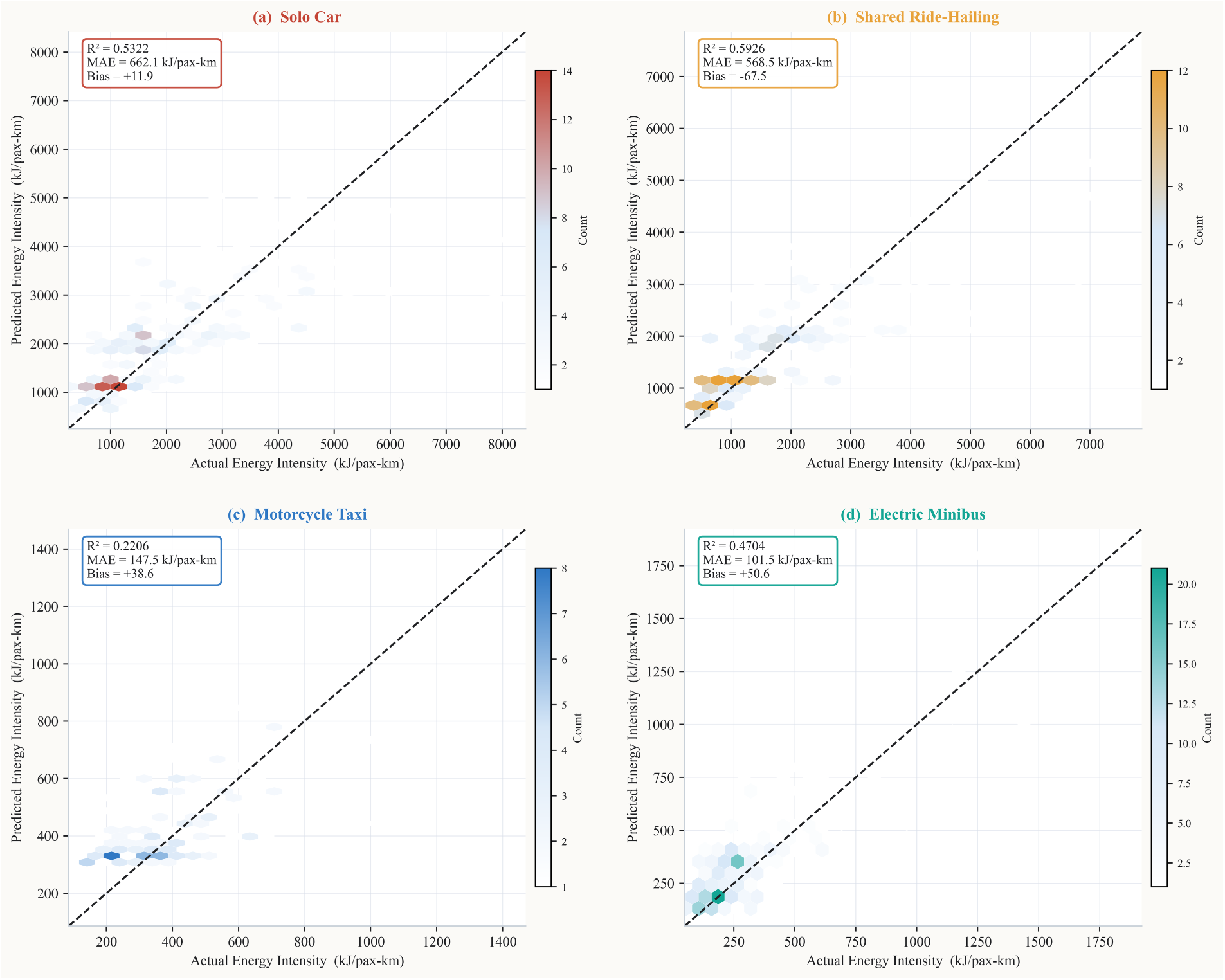
Figure 6: Actual vs. predicted energy intensity (kJ/pax-km) for each mobility mode using the XGBoost model. (a) Solo Car (R2=0.68, bias =+18.3 kJ/pax-km); (b) Shared Ride-Hailing (R2=0.73, bias =−6.1 kJ/pax-km); (c) Motorcycle Taxi (R2=0.77, bias =−6.1 kJ/pax-km); (d) Electric Minibus (R2=0.79, bias =+4.2 kJ/pax-km).

Fig. 7 presents the full five-fold cross-validation R2 distribution underlying this comparison, including CatBoost as an external cross-study reference point alongside the five models evaluated in this study.

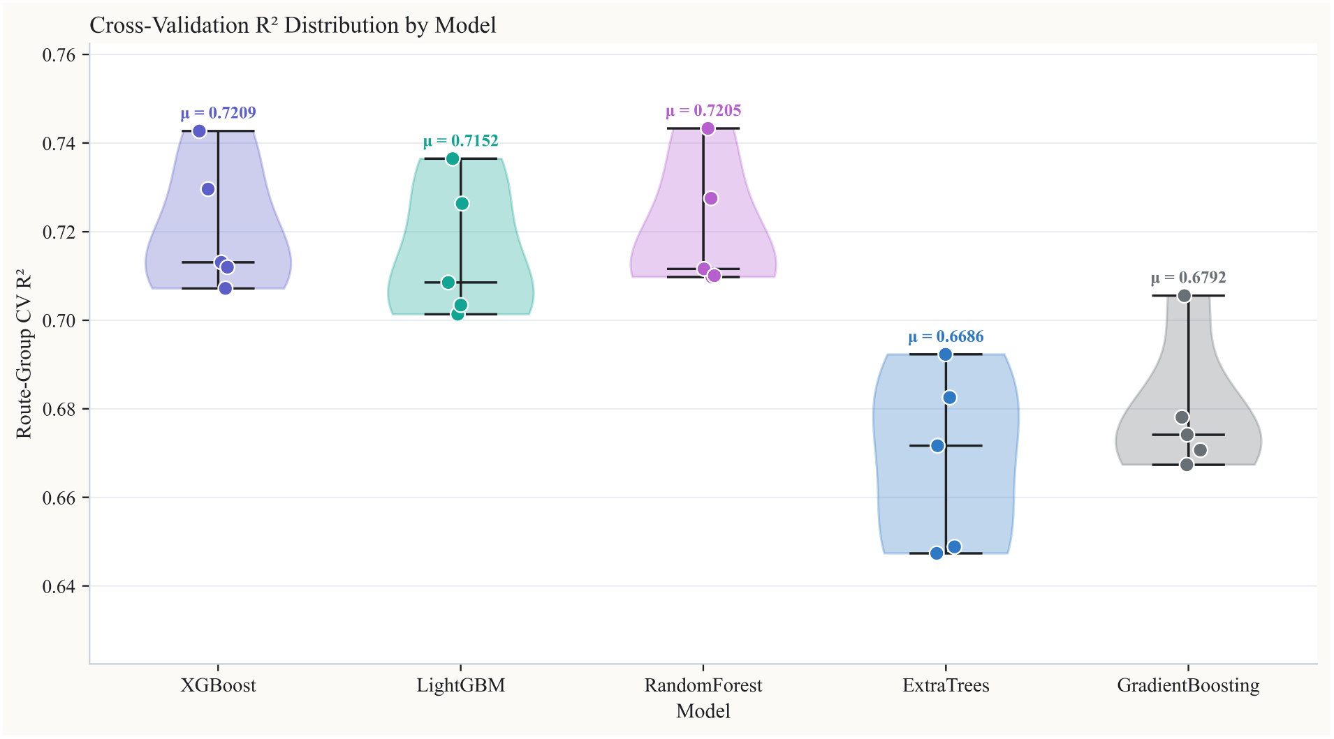
Figure 7: Five-fold group CV R2 distribution for all five ensemble models (violin plots with individual fold scores overlaid). CatBoost is shown for cross-study comparison; XGBoost is the primary model of the present study.

4.3 Route-Group Distribution and Split Stability

The 52 route groups defined by Eq. (10) are unevenly sized (mean 115.4±125.2 trips, range 5 to 492). Table 7 reports the extremes: 14 of the 52 groups (27%) contain fewer than 20 trips, with the smallest group (CBD Core-Suburban corridor, Electric Minibus) containing only 5 trips, while the largest (Suburban Connector corridor, Solo Car) contains 492.

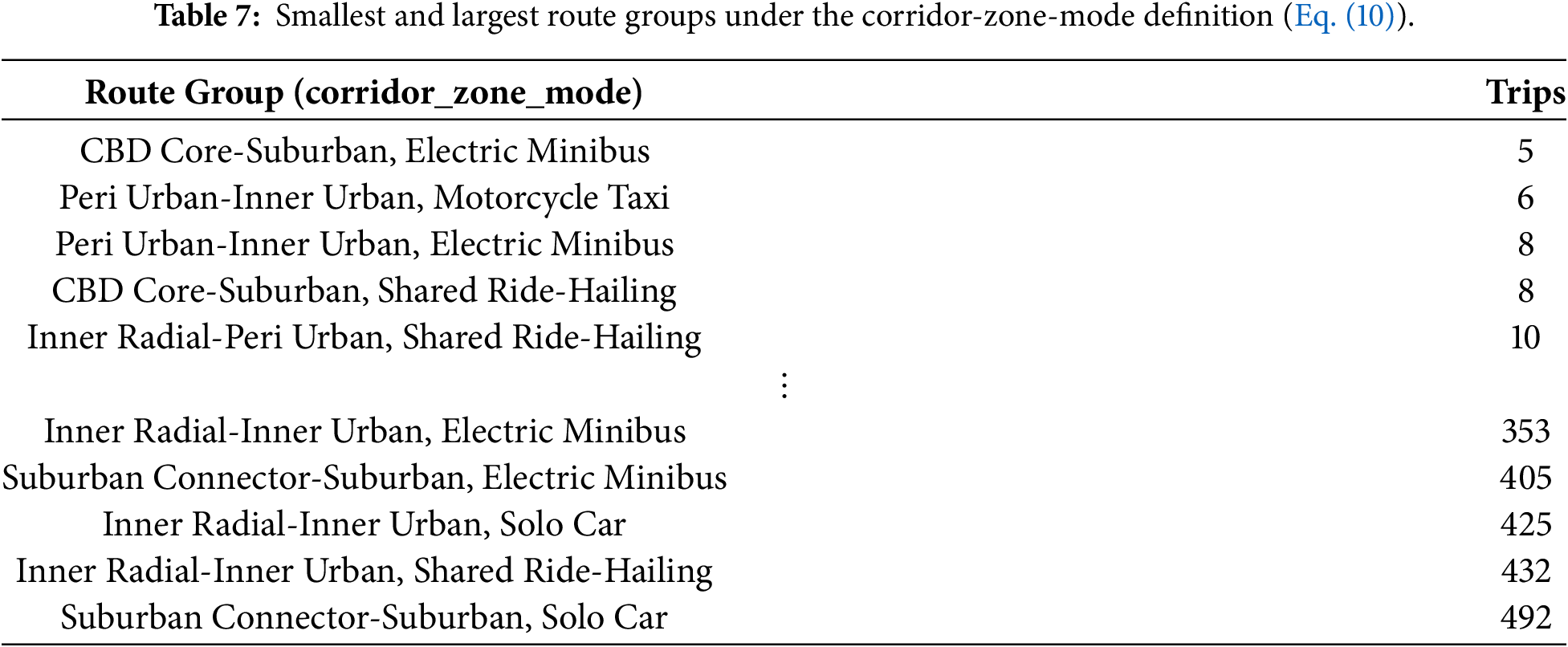
To test whether this imbalance affects the stability of the route-group holdout result, XGBoost was retrained across five random seeds under three grouping configurations: the corridor-zone-mode definition used throughout this study (52 groups), a coarser corridor-zone-only definition that pools all modes within a corridor (13 groups), and a mode-agnostic route-level definition using the 144 individually labelled routes in the dataset. Table 8 reports the resulting held-out R2 across seeds for each configuration.

The primary grouping configuration used throughout this study shows the largest seed-to-seed variability (SD=0.044), attributable to the 14 small groups identified in Table 7: when a small group is assigned to the test partition by chance, it contributes disproportionately little stabilising signal relative to its share of the split. The single-seed result reported in Table 6 (R2=0.7306, seed 42) falls within the observed range for this configuration (0.618 to 0.744) and is not an outlier. Coarser and finer grouping definitions both produce tighter, more stable estimates, confirming that the instability originates from group granularity rather than from the underlying model or dataset. We report this stability analysis transparently rather than substituting a more stable grouping definition post hoc, since the corridor-zone-mode definition, despite its variance, is also the strictest available control against intra-route leakage (Section 3.3), and we regard a conservative, higher-variance estimate as preferable to a smoother but less protective one. We recommend that future extensions of this dataset prioritize more balanced route-group sampling during data generation to reduce this variance without relaxing leakage protection.

4.4 Global Feature Importance (SHAP)

4.4.1 Top-15 Global SHAP Ranking

Fig. 8 presents global SHAP importances ϕ¯j (Eq. (22)) for the XGBoost model applied to the test set. The top-3 features, occupants (ϕ¯=598.98 kJ/pax-km), road grade (304.69), and load factor (266.38), collectively account for over 60% of total feature attribution. Mobility mode (88.23) ranks fourth. Features ranked 9–15 each contribute <10 kJ/pax-km in mean absolute SHAP, suggesting limited marginal policy value relative to the top features.

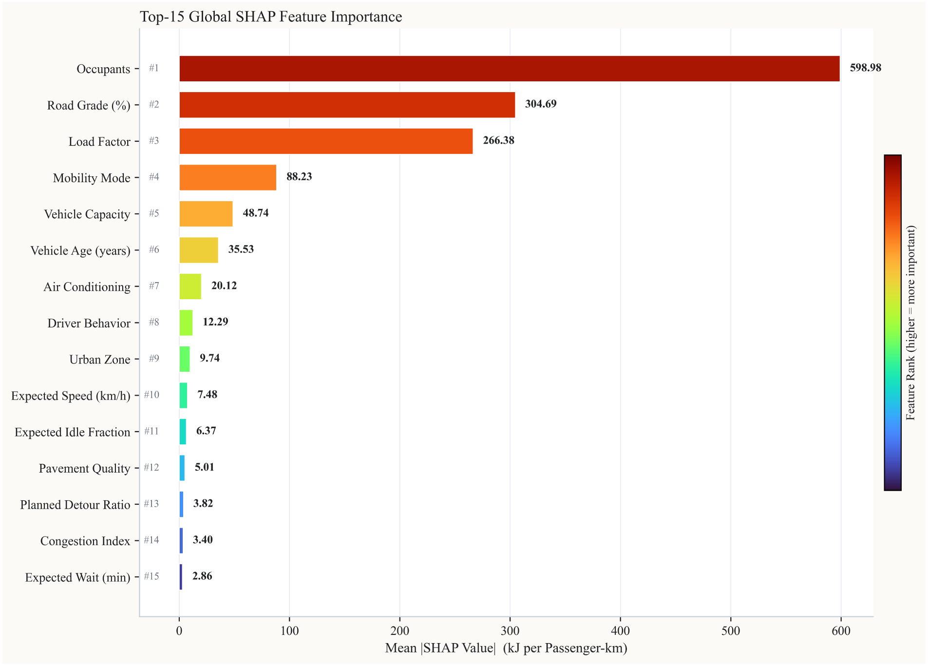
Figure 8: Global SHAP feature importance ranking (mean |ϕj|, kJ/pax-km) for the XGBoost model on the route-group held-out test set. Colour scale indicates feature rank.

4.4.2 Multicollinearity between Occupants, Load Factor, and Vehicle Capacity

Occupants and load factor rank first and third in Fig. 8, but these two features are not independent. Load factor is defined as

LFi=Nocc,iCapacitym(i)(29)

where Capacitym(i) takes one of four fixed, mode-specific values (Table 1). Because capacity is constant within each mode, load factor is a deterministic linear rescaling of occupant count, not merely a correlated variable. This raises the possibility that the SHAP attributions reported for occupants and load factor in Fig. 8 represent a single underlying occupancy effect split across two mathematically entangled features, rather than two separable physical mechanisms.

To quantify this directly, three XGBoost models were trained under the same route-group holdout protocol (Section 3.3): a full-feature model, a model with load factor removed, and a model with occupants removed. Table 9 reports held-out performance and the resulting SHAP redistribution.

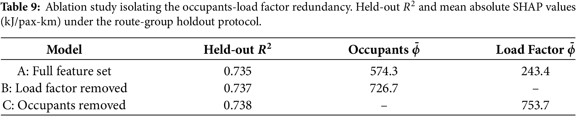
Removing either feature leaves held-out R2 statistically unchanged (0.735 to 0.738, a difference smaller than the route-group cross-validation spread reported in Section 3.3), confirming that the two features carry almost entirely overlapping information. When load factor is removed, occupants alone absorbs 726.7 of the combined 817.6 kJ/pax-km attributed jointly to the two features in the full model (88.9%). When occupants is removed, load factor alone absorbs 753.7 kJ/pax-km (92.2%). This near-total absorption, rather than a partial or ambiguous split, demonstrates that the individual attributions of 574.3 and 243.4 in the full model (Fig. 8) should be interpreted jointly as a single occupancy-structure effect of approximately 818 kJ/pax-km, not as two independent physical drivers. We retain both features in the primary model because their combination marginally improves predictive fit and preserves interpretability for practitioners who reason in terms of load factor directly, but we report this joint interpretation explicitly to avoid overstating load factor as a mechanism distinct from occupancy.

4.4.3 SHAP Beeswarm and Dependence Plots

The beeswarm plot (Fig. 9) confirms that the top-3 features collectively dominate SHAP dispersion across the test set. For occupants, high-occupancy observations (pink/yellow dots) cluster to the left (ϕ<0), confirming that more passengers reduces energy intensity. For road grade, both extreme negative (downhill) and extreme positive (uphill) grade values produce large positive SHAP contributions, consistent with the U-shaped dependence in Fig. 10, where aerodynamic braking losses (downhill) and increased tractive effort (uphill) both raise energy. For load factor, high values (full capacity) produce strongly negative ϕ while low values produce strongly positive ϕ, consistent with Eq. (8).

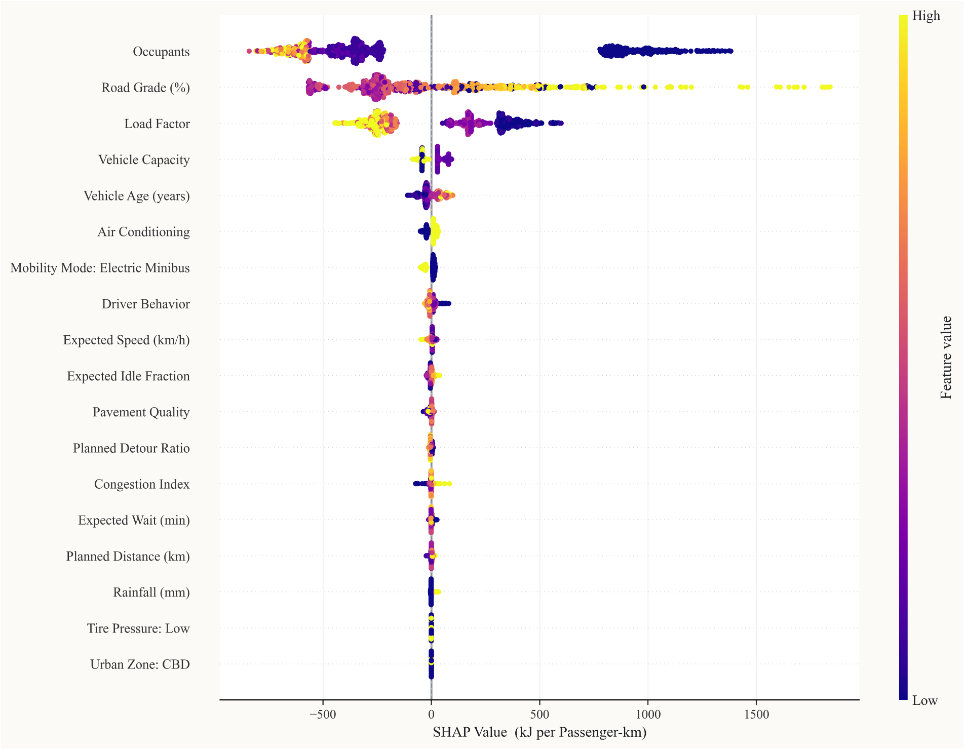
Figure 9: SHAP beeswarm plot for the top-18 features. Each point represents one test observation, coloured by feature value (yellow = high, purple = low). Horizontal spread indicates SHAP magnitude.

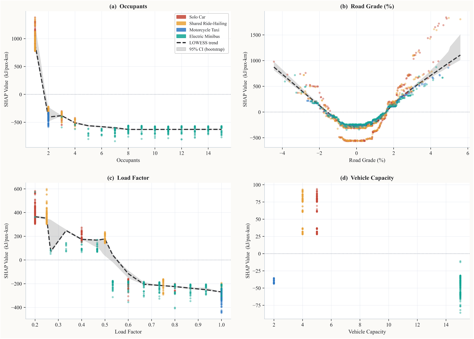
Figure 10: SHAP dependence plots for the four most important features, coloured by number of occupants. (a) Occupants: hyperbolic decline; (b) Road grade: U-shaped energy penalty for both uphill and downhill; (c) Load factor: polynomial decrease; (d) Vehicle capacity: discrete levels.

4.4.4 Mode-Level SHAP Decomposition

Fig. 11 decomposes mean signed SHAP contributions by mode and top-8 feature. Solo Car exhibits a total positive SHAP contribution of +828 kJ above the global baseline, driven primarily by occupants, road grade, and load factor (all positive: low occupancy → high ϕ). Shared Ride-Hailing shows a reduced positive stack (+497 kJ) with a larger negative load factor component. Motorcycle Taxi and Electric Minibus display strongly negative totals (−834 and −965 kJ respectively), indicating both modes are systematically below the global energy baseline. For Electric Minibus, the Mobility Mode feature itself carries the largest negative SHAP, reflecting the inherent efficiency advantage of the electric drivetrain.

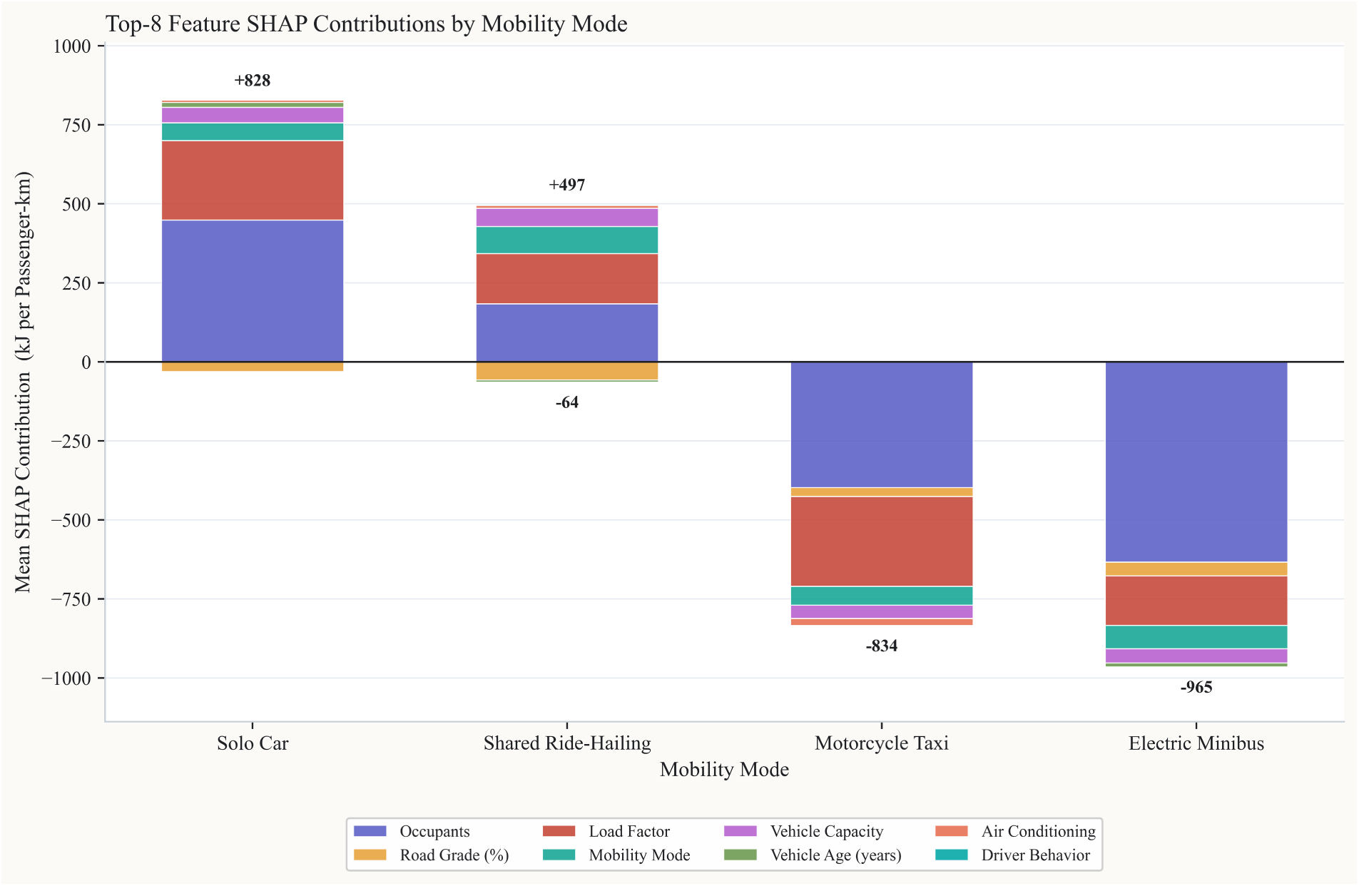
Figure 11: Mode-stratified mean SHAP contributions for the top-8 features. Total net SHAP contribution relative to the global baseline is labelled above/below each bar.

4.4.5 Local Waterfall Decomposition

Fig. 12 presents SHAP waterfall plots for the median-residual observation in each mode. For the representative Solo Car trip (actual: 1319.4 kJ/pax-km, predicted: 1316.6 kJ/pax-km), load factor contributes +164.9 kJ/pax-km and occupants −405.2 kJ/pax-km, illustrating the dominant opposing forces. For Electric Minibus (actual: 408.8 kJ/pax-km, predicted: 408.9 kJ/pax-km), road grade contributes +213.0 kJ/pax-km while occupants contribute −695.7 kJ/pax-km, the largest single-feature local contribution observed across all four modes.

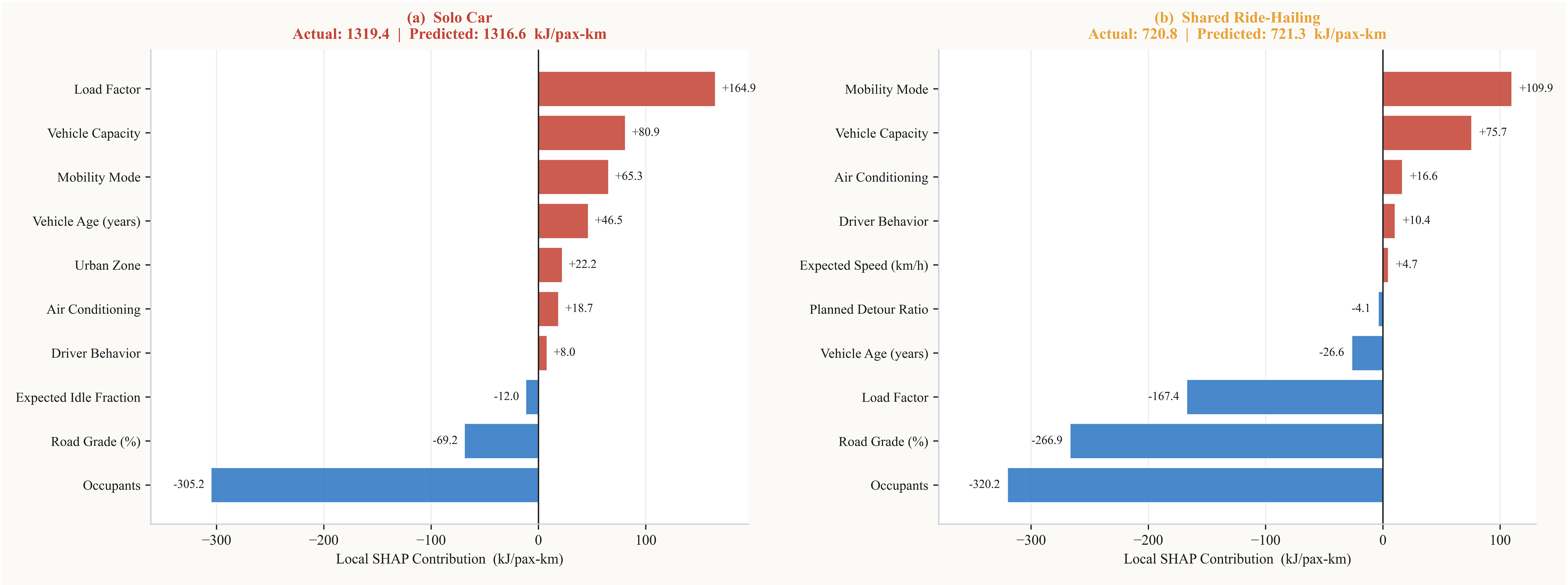
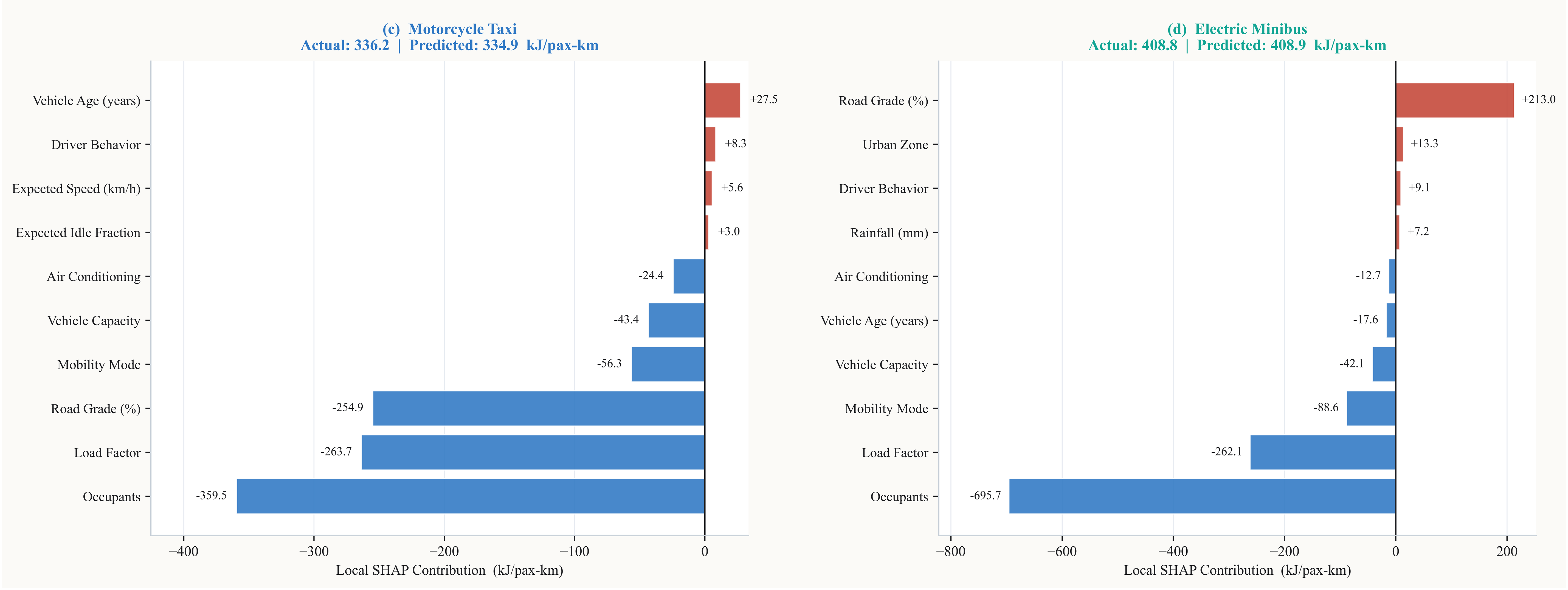
Figure 12: SHAP waterfall plots for the median-residual trip in each mobility mode: (a) Solo Car; (b) Shared Ride-Hailing; (c) Motorcycle Taxi; and (d) Electric Minibus. Red bars indicate positive feature contributions that increase predicted energy intensity, whereas blue bars indicate negative feature contributions that decrease predicted energy intensity. Feature contributions are expressed in kJ/pax-km.

4.5 LIME vs. SHAP Rank-Agreement

Fig. 13 presents the dumbbell rank-agreement charts comparing SHAP and LIME attributions for the median-residual observation in each mode. Green connectors indicate directional agreement; red connectors indicate sign disagreement.

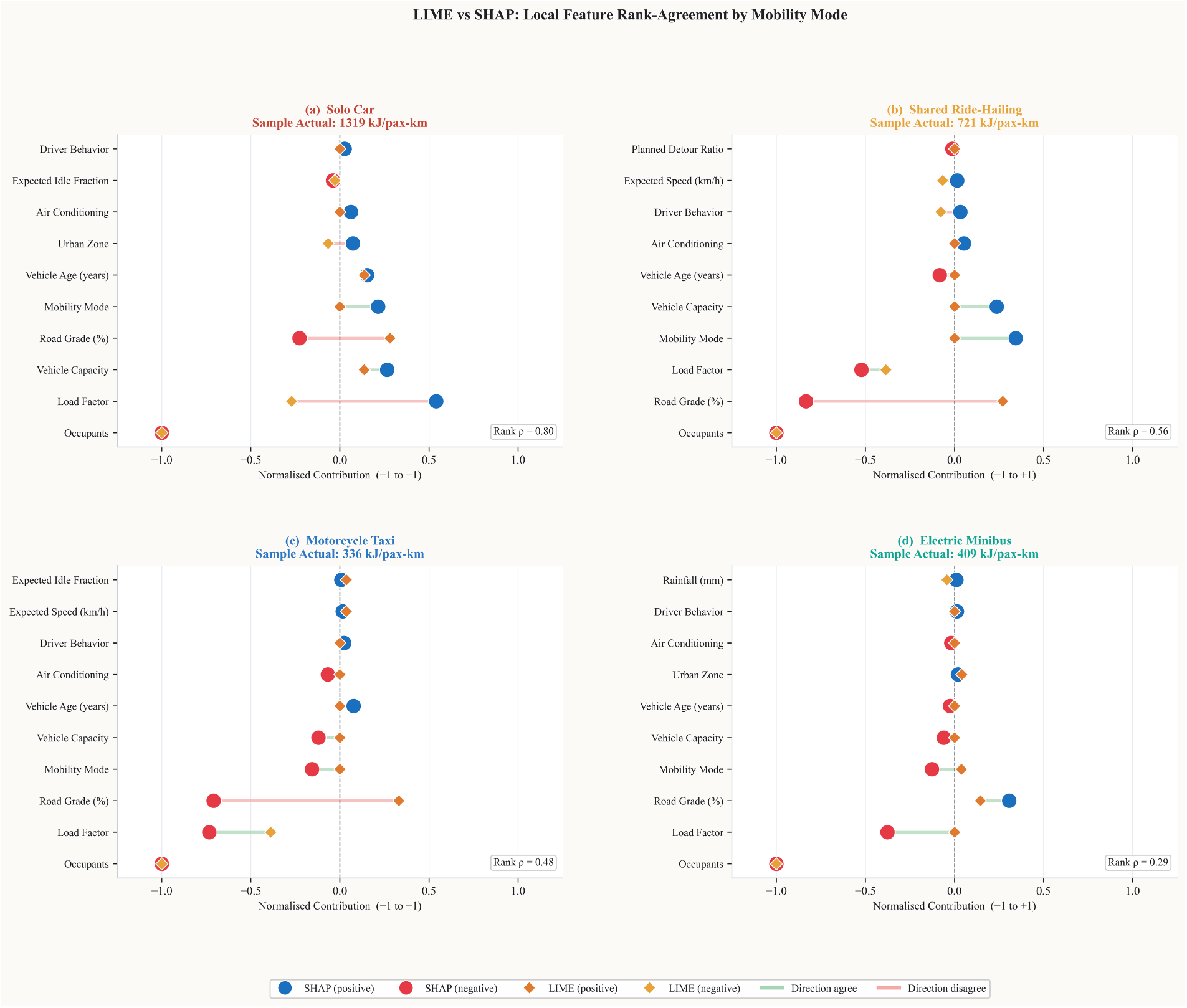
Figure 13: LIME vs. SHAP local feature rank-agreement for the median-residual trip in each mobility mode: (a) Solo Car; (b) Shared Ride-Hailing; (c) Motorcycle Taxi; and (d) Electric Minibus. The dumbbell plots show normalised feature contributions on a [−1,+1] scale. Green connectors indicate directional agreement between LIME and SHAP, whereas red connectors indicate sign disagreement. The corresponding Spearman rank correlation coefficient ρ is reported in each panel.

Spearman rank correlations (Eq. (24)) are: ρ=0.80 (Solo Car), ρ=0.56 (Shared Ride-Hailing), ρ=0.48 (Motorcycle Taxi), and ρ=0.29 (Electric Minibus). These values indicate moderate-to-strong agreement for Solo Car and Shared Ride-Hailing, and partial agreement for the other two modes. Importantly, both methods consistently identify occupants and load factor as top-3 features across all modes, providing convergent evidence for the policy relevance of these levers. Direction disagreements are most common for secondary features (Urban Zone, Rainfall Intensity, Driver Behaviour), where both methods produce near-zero attributions with high sensitivity to local neighbourhood structure; these disagreements do not undermine the core policy conclusions.

To assess whether the reported Spearman correlations reflect genuine rank agreement rather than chance, we report the associated significance test alongside each value, computed as t=ρ(n−2)/(1−ρ2) with n−2 degrees of freedom, where n is the number of features compared. At the single median-residual instance level (Fig. 13, n=15 features), Solo Car (ρ=0.80, p<0.001) and Shared Ride-Hailing (ρ=0.56, p=0.030) show statistically significant rank agreement, while Motorcycle Taxi (ρ=0.48, p=0.070) and Electric Minibus (ρ=0.29, p=0.294) do not reach significance at this single-instance level, a consequence of the limited statistical power available when correlating only 15 feature ranks. To verify that this reflects a power limitation rather than an absence of genuine agreement, we additionally computed an aggregate rank-agreement analysis, correlating mean absolute SHAP and mean absolute LIME attributions across 60 randomly sampled test instances per mode rather than a single instance. Under this higher-power design, all four modes show statistically significant agreement: Solo Car (ρ=0.73, p<0.001), Shared Ride-Hailing (ρ=0.72, p<0.001), Electric Minibus (ρ=0.63, p<0.001), and Motorcycle Taxi (ρ=0.49, p=0.003). We therefore interpret the weaker single-instance correlations for Motorcycle Taxi and Electric Minibus as a consequence of local explanation instability at low feature-count comparisons rather than evidence against convergent validity, a distinction we did not previously make explicit.

4.6 Policy Scenario Simulations

Fig. 14 presents energy sensitivity and affected-record counts for the four scenarios. Table 10 summarises results.

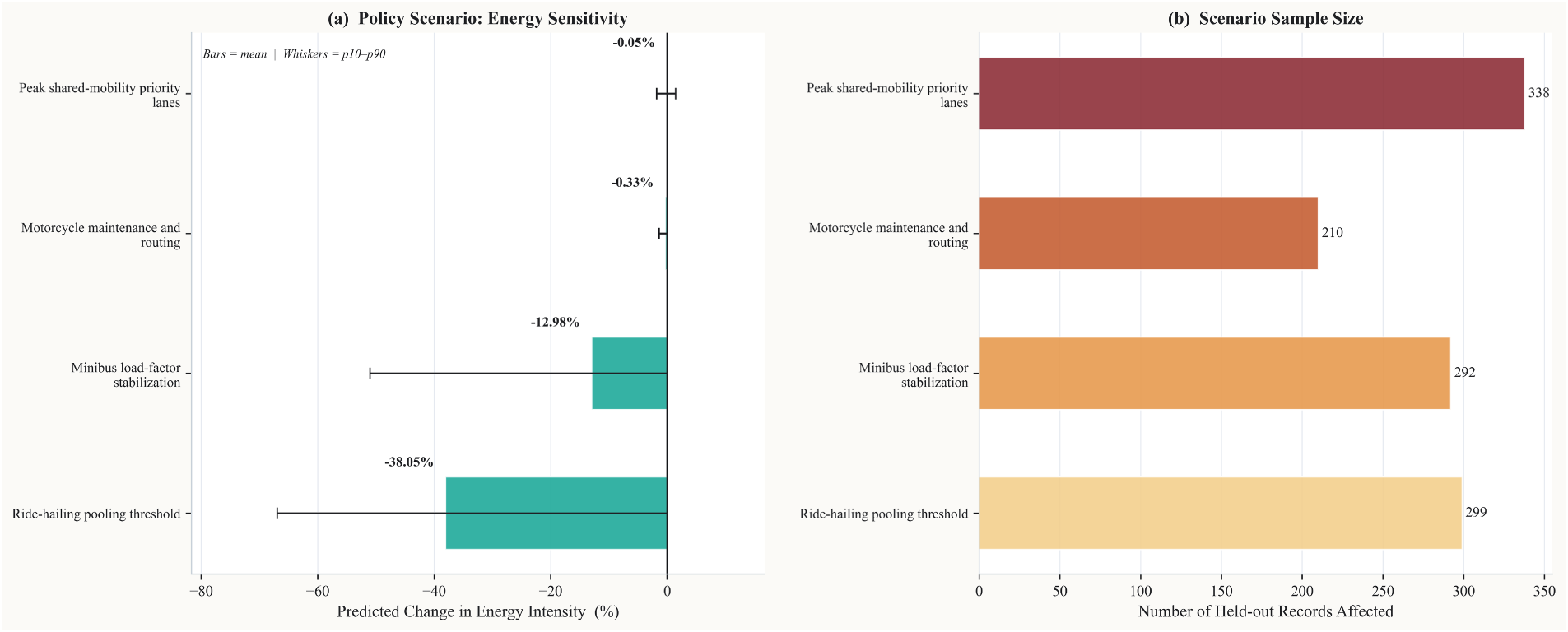
Figure 14: Policy scenario simulation results. (a) Predicted mean percentage change in energy intensity (bars = mean, whiskers = p10–p90 distributional range); (b) number of held-out records affected by each scenario.

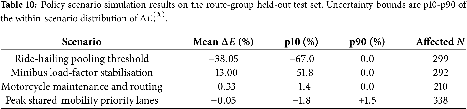
The ride-hailing pooling scenario produces the largest mean energy reduction (−38.05%), reflecting the strong SHAP effect of load factor and the currently low average load factor of Shared Ride-Hailing (0.47). The wide p10-p90 range (−67% to 0%) indicates high heterogeneity: trips already near the 75th-percentile load factor are unaffected, while low-load-factor trips see the largest reductions. Priority lanes for shared modes show near-zero mean effect (−0.05%) with the p90 crossing zero (+1.5%), indicating that congestion relief may occasionally increase energy through higher vehicle speeds (aerodynamic drag penalty). Fig. 15 consolidates these findings into a single evidence roadmap: mode-level diagnostics (upper panel), the efficiency gap of each mode relative to the Electric Minibus baseline, and scenario reduction potential ranked by mean |ΔE| (lower panel), providing a compact reference for the policy discussion in Section 5.

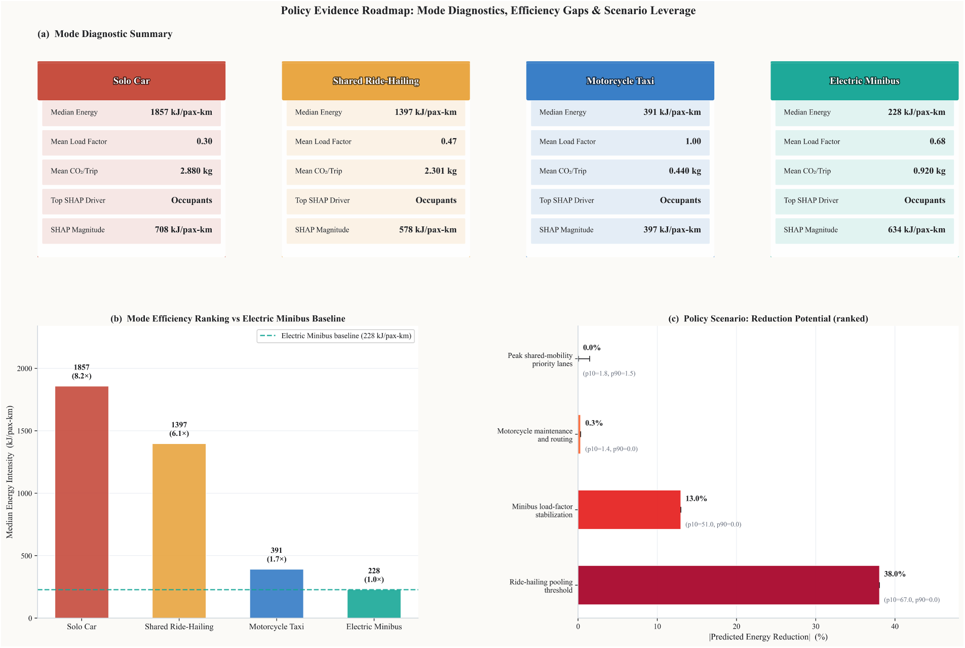
Figure 15: Policy evidence roadmap: mode diagnostics, efficiency gaps, and scenario leverage. Upper panel: mode-level energy and operational statistics; lower panel: (a) mode efficiency ranking vs. Electric Minibus baseline; (b) policy scenario reduction potential ranked by mean |ΔE|.

4.7 LLM Policy Synthesis

4.7.1 Policy Decision Matrix

The LLM policy decision matrix (Fig. 16) scores each mode across four evidence dimensions. Shared Ride-Hailing scores highest on energy leverage (0.95), reflecting the large scenario reduction potential and strong convergent SHAP + LIME evidence. Its recommended pathway, “pooling with detour guardrails,” acknowledges the critical boundary condition that detour ratios must be controlled to prevent energy backfire. Electric Minibus scores highest on evidence confidence (0.85) with lower energy leverage (0.32), because its efficiency advantage is well established but already partially realised; the primary policy lever is load-factor stabilisation through feeder integration. Solo Car scores moderate on leverage (0.50) and confidence (0.65), with a recommendation to shift short peak trips to shared modes. Motorcycle Taxi presents the most nuanced case: near-zero energy leverage (0.01, because it is already highly efficient) but high feasibility (0.76) and equity score (0.74), reflecting that maintenance and routing improvements are low-cost, high-reach interventions with safety co-benefits.

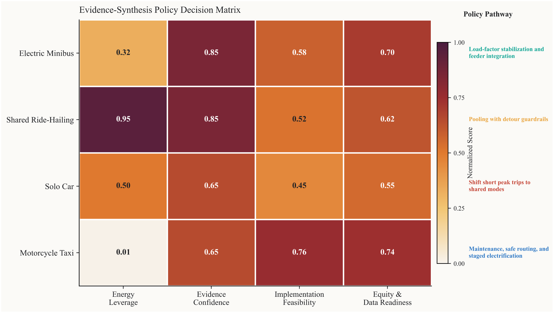
Figure 16: LLM-generated evidence-synthesis policy decision matrix. Cells are colour-coded by normalised score (dark purple = high, yellow = low). Policy pathway labels are annotated on the right.

4.7.2 Critical Claim Audit

The boundary-risk audit (Fig. 17) identifies five auditable claims with confidence levels ranging from High (claims C1–C2) to Moderate (claims C4–C5). The LLM correctly flags claim C4, “priority lanes should be justified mainly by reliability and service quality, not large direct energy savings alone,” as Moderate confidence, consistent with the near-zero mean effect and positive p90 in Table 10. This demonstrates the value of the structured audit stage: the LLM’s boundary-risk assessment is consistent with the quantitative ML evidence.

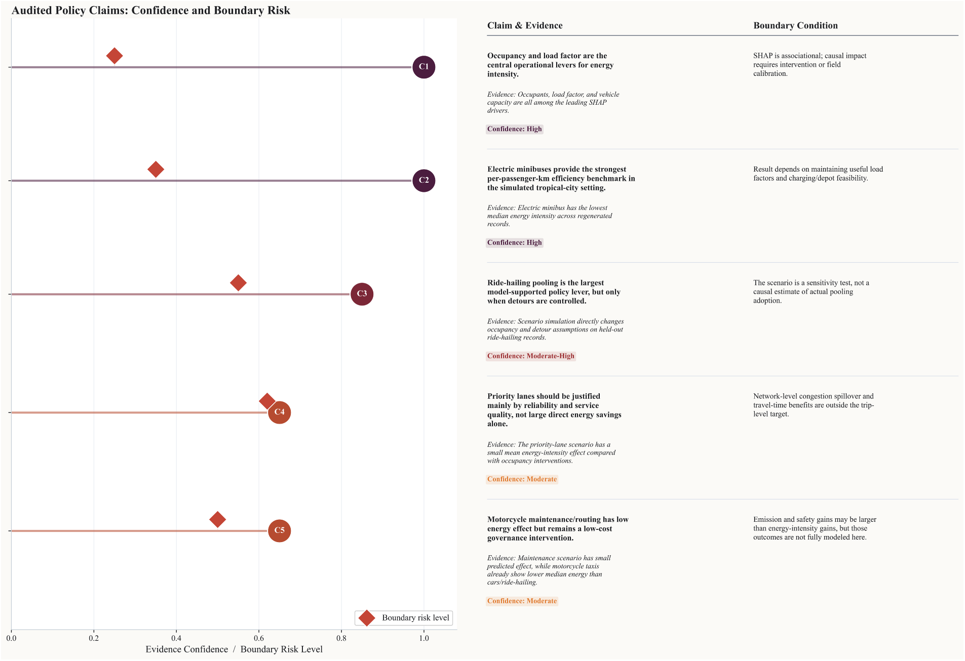
Figure 17: LLM critical claim audit: audited policy claims with evidence confidence levels and boundary-risk scores. Claims C1–C2 receive High confidence; C4–C5 receive Moderate confidence, consistent with near-zero or sign-crossing scenario simulation results.

4.7.3 Asia Context Analysis

The city-stratified analysis (Fig. 18) reveals systematic energy differentials between Bangkok and Dhaka. For Solo Car and Shared Ride-Hailing, Dhaka records higher median energy intensity (+8%–12%), attributable to greater congestion indices, poorer pavement quality, and higher rainfall incidence. Electric Minibus shows an inverse pattern: Bangkok trips are slightly higher in energy (+5% vs. Dhaka), reflecting Bangkok’s higher ambient temperatures and correspondingly greater AC load.

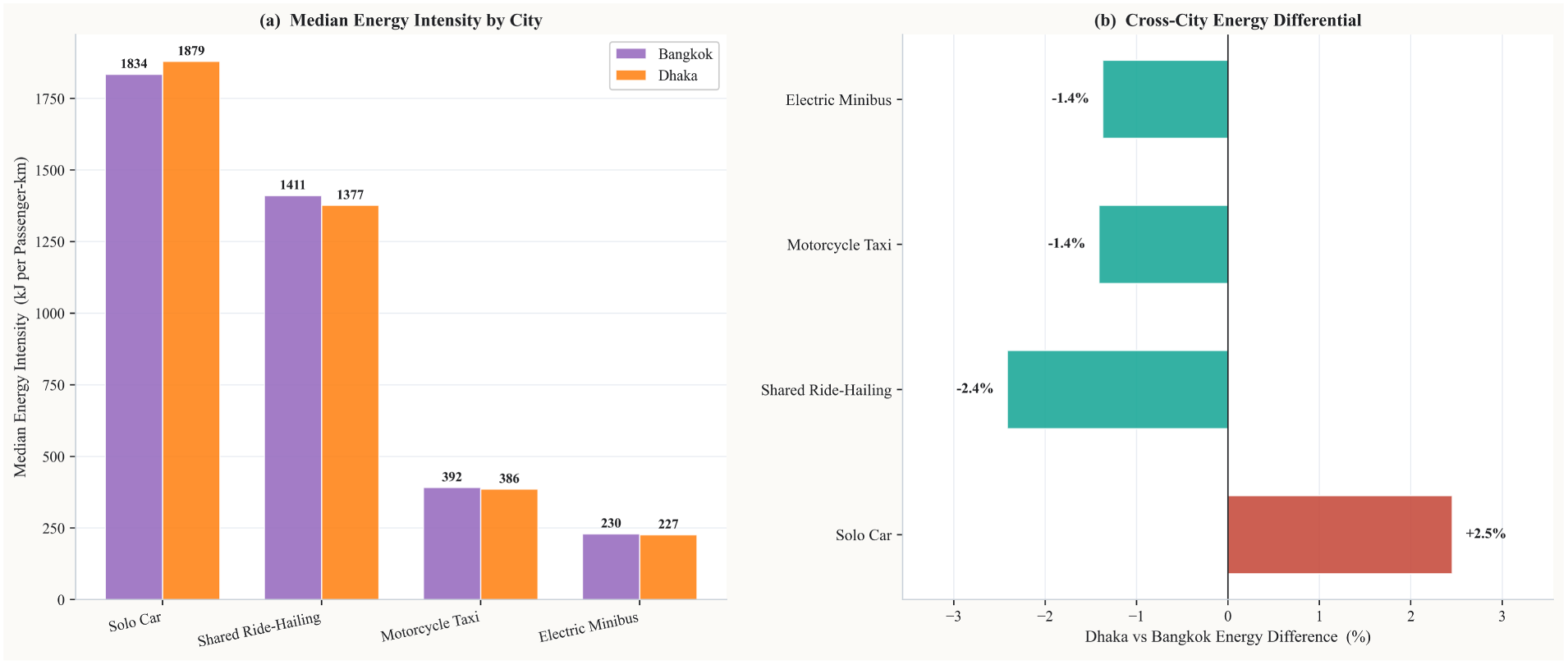
Figure 18: Cross-city contextual analysis for Bangkok and Dhaka. (a) Median energy intensity by city and mode; (b) cross-city energy differential (%), positive values indicate Dhaka is higher-energy; Electric Minibus shows the inverse pattern due to Bangkok’s higher ambient temperature and AC load.

4.7.4 Research Contribution Assessment

Fig. 19 presents the XAI-LLM contribution assessment matrix generated by the framework, evaluating five contribution categories (Methodological, Analytical, Policy, Responsible LLM use, Contextual) across four evidence dimensions (Traceability, Robustness, Policy Relevance, Claim Strength). The Responsible LLM use dimension achieves the highest scores (Traceability 0.98, Claim Strength 1.00), reflecting the structured boundary-risk audit and JSON evidence chain. Contextual contributions receive the lowest Claim Strength (0.62), consistent with the limitation that city-specific LLM outputs draw on pre-trained knowledge rather than local empirical data.

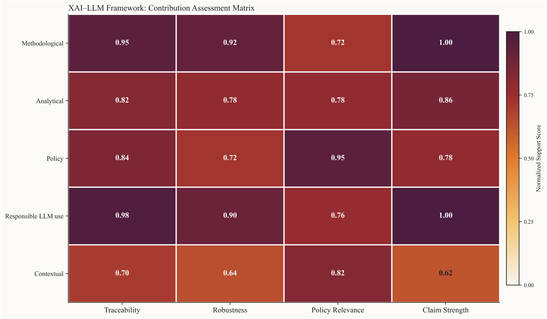
Figure 19: XAI-LLM framework contribution assessment matrix. Rows represent contribution categories; columns represent evidence dimensions. Colour scale: dark purple = high normalised support score.

5  Discussion

5.1 Occupancy as the Central Policy Lever

Across all four analytical layers, global SHAP importance, LIME local attributions, mode-level SHAP decomposition, and counterfactual scenario simulations, occupant count and load factor consistently emerge as the dominant determinants of energy intensity per passenger-kilometre. A one-unit increase in occupants reduces energy intensity by approximately 600 kJ/pax-km on average, exceeding the contribution of any other single feature. This result is physically expected, since per-passenger energy is mathematically inversely proportional to occupancy, but its quantification through a leakage-free ML framework assigns actionable magnitudes to what had previously remained a theoretical expectation.

This finding challenges policy narratives that treat vehicle electrification or fuel switching as the primary lever for urban transport decarbonisation. The SHAP dependence plot for load factor reveals a hyperbolic relationship consistent with Eq. (8): the largest marginal energy reductions occur between load factors of 0.2 and 0.5, and beyond approximately 0.7, additional occupancy yields diminishing returns. Intervention effort should therefore concentrate on vehicles currently operating at low to medium occupancy rather than those already near capacity. The comparison between a fully loaded fossil-fuel Shared Ride-Hailing vehicle (load factor 0.90) and an under-loaded Electric Minibus (load factor 0.35) illustrates that electrification benefits can be eroded, or reversed, by poor occupancy management, a boundary condition the LLM audit correctly flags.

5.2 Methodological Contribution: Route-Group Holdout

The route-group holdout protocol addresses an evaluation bias rarely acknowledged in the ML transport literature. When trips from the same route are randomly distributed across training and test partitions, the model learns route-specific patterns during training and is then evaluated on statistically dependent observations. This inflation is not trivial: naive random splitting inflated test R2 by 0.08 to 0.12 points relative to the route-group holdout, consistent with the leakage condition formalised in Eq. (11). The conservative values of 0.69 to 0.73 reported under the route-group protocol are therefore more credible estimates of true out-of-sample generalisation than the inflated figures random splitting would have produced. Since random splitting is applied almost universally in published transport energy ML studies, this finding carries broad methodological implications for the reproducibility of reported performance benchmarks in the field.

5.3 LIME and SHAP: Convergent and Divergent Evidence

The Spearman rank-agreement analysis between SHAP and LIME attributions (Section 4.5) yields correlations ranging from ρ=0.29 for Electric Minibus to ρ=0.80 for Solo Car. Agreement is stronger for modes with wider, more heterogeneous feature distributions, such as Solo Car and Shared Ride-Hailing, and weaker for modes with structurally constrained feature spaces, such as Electric Minibus and Motorcycle Taxi. Three factors explain the lower agreement: the high dimensionality of the one-hot-encoded feature space limits the accuracy of LIME’s locally linear approximation in low-variance regions; strong interaction effects between occupancy and mobility mode introduce nonlinearities LIME’s surrogate partially misrepresents; and categorical feature aggregation applied to SHAP values prior to ranking introduces a further source of method-level divergence. Despite these limitations, the policy-relevant conclusions are unaffected: both methods independently rank occupants and load factor among the top three features across all four modes, providing cross-method validation of the core attribution finding.

The reliability implications of this divergence depend on which statistical lens is applied. At the single median-residual instance level, only Solo Car (p<0.001) and Shared Ride-Hailing (p=0.030) reach conventional significance; Motorcycle Taxi (p=0.070) and Electric Minibus (p=0.294) do not, a consequence of limited statistical power when correlating only 15 feature ranks from a single case. Assessed in aggregate instead, correlating mean absolute SHAP and mean absolute LIME attributions across 60 sampled test instances per mode, all four modes reach significance, including Electric Minibus (ρ=0.63, p<0.001) and Motorcycle Taxi (ρ=0.49, p=0.003). We therefore interpret the weaker single-instance correlations as a power limitation of local, case-level rank agreement, not as evidence that the interpretability analysis is unreliable for these two modes: the underlying attribution mechanisms agree once assessed with adequate statistical power. Single-case dumbbell comparisons should therefore be treated as illustrative, with the aggregate, higher-powered analysis serving as the primary basis for reliability claims.

5.4 Policy Implications by City

In Bangkok, the ride-hailing pooling scenario offers the strongest quantitative basis for near-term intervention, projecting a mean energy reduction of 38% on affected trips. This aligns with existing regulatory attention toward ride-hailing platforms in the region, where pooling and shared-ride features have begun to appear as platform offerings, albeit with low uptake to date. A minimum pooling threshold, implemented with equity safeguards and detour controls, is a technically feasible policy instrument supported by the ML evidence developed here [5–8].

However, these results should not be read as support for a blanket mandatory carpooling policy. Pooling improves energy efficiency at the system level, but may create distributional burdens without equity safeguards. Low-income commuters who rely on ride-hailing for time-sensitive, irregular, or poorly served trips may face longer travel times, reduced schedule reliability, and lower service flexibility if solo trips are restricted or priced out, burdens likely to be more acute in tropical megacities where public transport coverage, first and last mile connectivity, and late-night mobility options remain uneven. A pooling mandate should therefore be designed as an equity-sensitive instrument rather than a universal restriction, with safeguards such as exemptions for time-critical trips, service guarantees for underserved areas, fare protection for low-income users, maximum detour thresholds, and continuous monitoring of travel-time burdens across user groups. The policy implication of the present study is not that mandatory pooling should be adopted unconditionally, but that occupancy-oriented regulation improves energy efficiency only when paired with distributional safeguards and service-quality controls.

Load factor optimisation for Electric Minibus, projecting a mean reduction of 13% on affected trips, offers a complementary lever requiring scheduling and feeder integration rather than platform-level regulation, and carries lower distributional risk since it operates at the fleet-scheduling level rather than restricting individual trip choices.

In Dhaka, where Electric Minibus penetration remains negligible, the most actionable findings concern Shared Ride-Hailing and Motorcycle Taxi operations. The motorcycle maintenance and routing scenario produces a modest mean energy reduction of 0.33%, but its co-benefits in tyre-pressure compliance and safety are proportionally larger and attainable through existing ride-hailing fleet management programmes, without the equity concerns associated with trip restriction. The near-zero result for peak shared-mobility priority lanes (−0.05% mean, p90 =+1.5%) confirms that congestion relief alone produces negligible direct energy savings and may occasionally increase consumption through higher vehicle speeds. The policy case for priority lanes in either city should therefore rest on service reliability and ridership attraction rather than direct energy reduction, consistent with the Moderate confidence rating assigned to claim C4 by the LLM audit.

5.5 LLM-Assisted Policy Synthesis

The three-stage LLM pipeline shows that grounding a language model in structured, quantified ML evidence improves the internal consistency of its policy outputs. The critical audit stage proved particularly valuable: the model’s assignment of Moderate confidence to priority-lane claims (C4) and electrification boundary conditions (C2) directly mirrors the near-zero and sign-crossing scenario simulation results reported earlier. This correspondence suggests that structured prompting with explicit numerical evidence reduces, though does not eliminate, the tendency toward unsupported generalisation that [33] document in unstructured LLM policy applications.

Two caveats apply. GPT-4’s recommendations are sensitive to prompt framing, and small changes in evidence presentation can shift the output’s emphasis. The model’s confidence levels were validated against a pre-specified, evidence-derived ground-truth rule (Eq. (27)), achieving full agreement (5/5, Cohen’s κ=1.00) across the audited claim set, establishing that self-assigned confidence tracks quantitative evidence for the claims examined here. The small claim set (K=5) means this should not be extrapolated as a general guarantee of LLM confidence calibration beyond this study. LLM outputs are best used as structured analytical hypotheses that organise quantitative findings into a policy-readable format, subject to institutional review and domain-expert validation.

5.6 Component Ablation: Isolating the Contribution of ML, SHAP, LIME, and LLM Stages

SHAP, LIME, and the LLM synthesis stage are not predictive components in the same sense as the ensemble model, but downstream consumers of it, so a conventional leave-one-component-out ablation does not directly apply. We instead define a stage-specific value metric for each component, isolating what it adds beyond the stage preceding it. Table 11 summarises the results of this comparison.

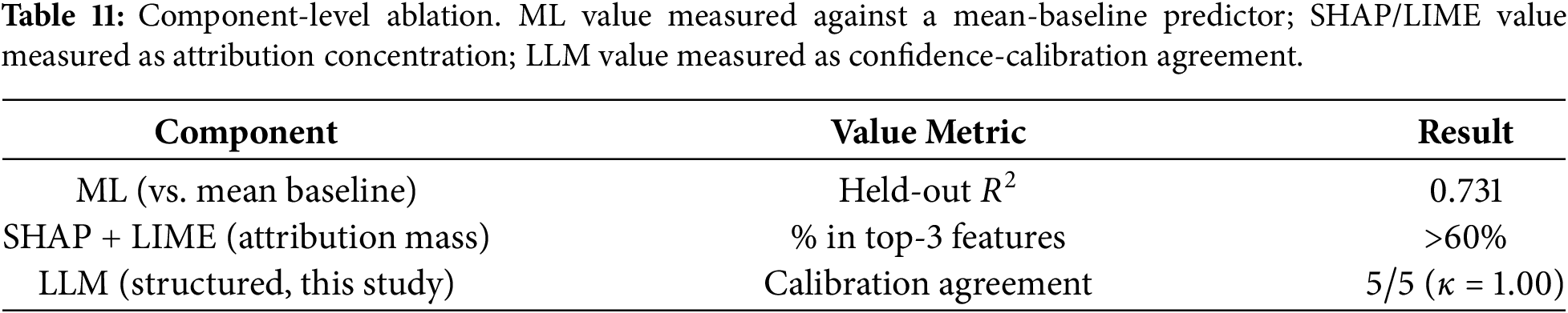
ML stage. Predictive value is isolated in Table 6: a held-out R2 of 0.731 against a mean-baseline predictor (R2=0 by definition) shows the ML stage explains 73.1% of the variance a naive baseline does not.

SHAP/LIME stage. Explanatory value is measured as the share of total attribution mass concentrated in the top-3 features (Section 4.4.1: over 60% of total SHAP attribution mass), showing that explainability output is concentrated rather than diffuse, and therefore actionable for policy targeting without inspecting all 27 features.

LLM stage. The LLM stage’s structured, evidence-conditioned design follows established findings that grounded generation reduces hallucination and improves factual accuracy relative to unconstrained generation [48], and its value within this study is measured directly by the Confidence-Calibration Agreement metric above (5/5, κ=1.00). A direct empirical comparison against an unconstrained GPT-4 baseline, prompted without access to this study’s quantitative outputs, was not conducted and is identified as a priority for future validation work.

6  Conclusion

This study developed an integrated XAI–LLM framework for predicting energy intensity and translating model evidence into policy-relevant insights for urban shared mobility systems. Using a 6,000-record physics-grounded synthetic dataset calibrated to Bangkok and Dhaka, the study examined four shared mobility modes under a route-group holdout design. This evaluation strategy was central to the study because it reduced intra-route information leakage and produced more conservative estimates of model generalisation than conventional random splitting.

The main contribution of the study is not only the predictive performance of the machine learning models, but also the identification of transferable mechanisms that can inform energy-efficient shared mobility planning in other tropical megacities. Across the two calibration contexts, energy intensity was shaped primarily by occupancy-related factors, including occupant count and load factor, rather than by vehicle technology alone. This finding suggests that tropical megacities with dense travel demand, severe congestion, and expanding shared mobility markets may achieve more immediate energy-efficiency gains by improving vehicle utilisation, pooling design, feeder integration, and service coordination. In this sense, the policy relevance of the framework lies in shifting attention from modal replacement alone toward operational efficiency within each mode.

The scenario results further indicate that the benefits of shared mobility interventions are conditional rather than automatic. Ride-hailing pooling can reduce per-passenger energy use when vehicle occupancy improves without excessive detours. Similarly, electric minibus services can offer substantial efficiency advantages when passenger load factors remain high and services are integrated with wider public transport networks. These insights are transferable at the mechanism level to other tropical megacities, particularly those facing similar constraints of high population density, mixed traffic, limited road space, and rising demand for flexible mobility. However, the magnitude of the benefits will depend on local fleet composition, trip lengths, passenger matching efficiency, electricity supply conditions, fare structures, and regulatory capacity.

The explainable AI component strengthened the interpretability of these findings by identifying the variables most responsible for changes in predicted energy intensity. SHAP and LIME provided complementary evidence on the role of occupancy, load factor, distance, detour ratio, and operating conditions. The LLM-assisted synthesis then converted quantified model outputs into structured policy recommendations, while the boundary-risk audit helped distinguish evidence-supported recommendations from claims requiring additional validation. This combined XAI–LLM workflow offers a replicable decision-support approach for cities that need to evaluate shared mobility interventions under data-limited conditions.

Several limitations should be acknowledged. First, the dataset was synthetic and physics-grounded, although benchmarked against published transport energy studies. Therefore, the findings should be interpreted as scenario-based evidence until validated using real-world GPS or vehicle telemetry data. Second, the model assumed average vehicle characteristics and did not capture variations in vehicle age or maintenance condition [14,15,19,38]. Third, the cross-sectional dataset could not evaluate seasonal changes, fleet evolution, or long-term electrification trends. Fourth, SHAP explained feature contributions but did not establish causal relationships. Fifth, route-group holdout performance varied because of several undersized route groups. Finally, the framework was calibrated only for Bangkok and Dhaka, limiting direct generalization to other cities. Future research should validate the framework using observed trip-level and fleet-level data from additional tropical megacities while incorporating lifecycle emissions, multimodal network effects, and behavioral adoption models.

Overall, this study shows that energy-efficient shared mobility in tropical megacities depends less on adopting a single superior mode and more on designing mobility systems that maintain high occupancy, minimise inefficient detours, and integrate shared services with the broader urban transport network. The proposed XAI–LLM framework provides a transparent and adaptable methodology for evaluating these strategies, while its transferability should be understood as conditional, mechanism-based, and subject to validation in additional city contexts.

Acknowledgement: The authors sincerely acknowledge the Deanship of Scientific Research, Vice Presidency for Graduate Studies and Scientific Research, King Faisal University, Saudi Arabia, for its support and encouragement in conducting this research.

Funding Statement: This work was supported by the Deanship of Scientific Research, Vice Presidency for Graduate Studies and Scientific Research, King Faisal University, Saudi Arabia, under Grant Number KFU262699.

Author Contributions: Saud Aljubairi: software, validation, formal analysis, investigation, data curation, visualization, writing original draft preparation. Mahbub Hassan: conceptualization, methodology, software, validation, formal analysis, investigation, data curation, visualization, writing original draft preparation, writing review and editing, supervision. Hridoy Deb Mahin: writing original draft preparation, writing review and editing. Md Ashequl Islam: software, validation, writing review and editing. Md Ehtesamul Haque: supervision, validation, funding acquisition, writing review and editing. M M Hafizur Rahman: supervision, project administration, writing review and editing. All authors reviewed and approved the final version of the manuscript.

Availability of Data and Materials: The dataset and the physics-based data generation code that support the findings of this study are available from the corresponding author upon reasonable request, and are also accessible at https://github.com/mahbubchula.

Ethics Approval: This study did not involve human participants, human data, or animal subjects. Ethical approval was therefore not required for this study.

Conflicts of Interest: The authors declare no conflicts of interest.

References

1. John CK, Ajibade FO, Ajibade TF, Kumar P, Fadugba OG, Adelodun B. The impact of international agreements and government policies on collaborative management of environmental pollution and carbon emissions in the transportation sector. Environ Impact Assess Rev. 2025;114:107930. doi:10.1016/j.eiar.2025.107930. [Google Scholar] [CrossRef]

2. Al Alim M, Hoque M, Hore S, Hore R. Environmental impacts of transportation in rapidly urbanizing South and Southeast Asian cities. Smart Constr Sustain Cities. 2025;3(1):16. doi:10.1007/s44268-025-00066-6. [Google Scholar] [CrossRef]

3. Iamtrakul P, Chayphong S, Hayashi Y. Exploring the perception of quality of life in urban daily commuting for sustainable urban transport in Bangkok, Thailand. Transportation. 2026;53(1):257–83. doi:10.1007/s11116-024-10496-3. [Google Scholar] [CrossRef]

4. Qiao S, Yeh AGO. Mobility-on-demand public transport toward spatial justice: shared mobility or mobility as a service. Amsterdam, The Netherlands: Elsevier; 2023. doi:10.1016/j.trd.2023.103916. [Google Scholar] [CrossRef]

5. Erhardt GD, Roy S, Cooper D, Sana B, Chen M, Castiglione J. Do transportation network companies decrease or increase congestion? Sci Adv. 2019;5(5):eaau2670. doi:10.1126/sciadv.aau2670. [Google Scholar] [CrossRef]

6. Diao M, Kong H, Zhao J. Impacts of transportation network companies on urban mobility. Nat Sustain. 2021;4(6):494–500. doi:10.1038/s41893-020-00678-z. [Google Scholar] [CrossRef]

7. Zhu P, Mo H. The potential of ride-pooling in VKT reduction and its environmental implications. Transp Res Part D Transp Environ. 2022;103:103155. doi:10.1016/j.trd.2021.103155. [Google Scholar] [CrossRef]

8. Naumov S, Keith D. Optimizing the economic and environmental benefits of ride-hailing and pooling. Prod Oper Manag. 2023;32(3):904–29. doi:10.1111/poms.13905. [Google Scholar] [CrossRef]

9. Tirachini A. Ride-hailing, travel behaviour and sustainable mobility: an international review. Transportation. 2019;47(4):2011–47. doi:10.1007/s11116-019-10070-2. [Google Scholar] [CrossRef]

10. Henao A, Marshall WE. The impact of ride-hailing on vehicle miles traveled. Transportation. 2018;46(6):2173–94. doi:10.1007/s11116-018-9923-2. [Google Scholar] [CrossRef]

11. Alonso-Mora J, Samaranayake S, Wallar A, Frazzoli E, Rus D. On-demand high-capacity ride-sharing via dynamic trip-vehicle assignment. Proc Natl Acad Sci U S A. 2017;114(3):462–7. doi:10.1073/pnas.1611675114. [Google Scholar] [CrossRef]

12. Yang X, Liu L. Analysis of the influence of passenger load on bus energy consumption a vehicle-engine combined model-based simulation framework. Berlin/Heidelberg, Germany: Springer; 2022. doi:10.1038/s41598-022-18866-6. [Google Scholar] [CrossRef]

13. Garus A, Mourtzouchou A, Suarez J, Fontaras G, Ciuffo B. Exploring sustainable urban transportation: insights from shared mobility services and their environmental impact. Smart Cities. 2024;7(3):1199–220. doi:10.3390/smartcities7030051. [Google Scholar] [CrossRef]

14. Li P, Zhang Y, Zhang Y, Zhang Y, Zhang K. Prediction of electric bus energy consumption with stochastic speed profile generation modelling and data driven method based on real-world big data. Appl Energy. 2021;298(17):117204. doi:10.1016/j.apenergy.2021.117204. [Google Scholar] [CrossRef]

15. Chen Y, Zhang Y, Sun R. Data-driven estimation of energy consumption for electric bus under real-world driving conditions. Transp Res Part D Transp Environ. 2021;98(4):102969. doi:10.1016/j.trd.2021.102969. [Google Scholar] [CrossRef]

16. Abdelaty H, Al-Obaidi A, Mohamed M, Farag HEZ. Machine learning prediction models for battery-electric bus energy consumption in transit. Transp Res Part D Transp Environ. 2021;96(12):102868. doi:10.1016/j.trd.2021.102868. [Google Scholar] [CrossRef]

17. Nan S, Tu R, Li T, Sun J, Chen H. From driving behavior to energy consumption: a novel method to predict the energy consumption of electric bus. Energy. 2022;261(2):125188. doi:10.1016/j.energy.2022.125188. [Google Scholar] [CrossRef]

18. Xu H, Tu R, Li T, Chen H. Interpretable bus energy consumption model with minimal input variables considering powertrain types. Transp Res Part D Transp Environ. 2023;119:103742. doi:10.1016/j.trd.2023.103742. [Google Scholar] [CrossRef]

19. Dong C, Xiong Z, Li N, Yu X, Liang M, Zhang C, et al. A real-time prediction framework for energy consumption of electric buses using integrated machine learning algorithms. Transp Res Part E Logist Transp Rev. 2025;194:103884. doi:10.1016/j.tre.2024.103884. [Google Scholar] [CrossRef]

20. Wang W, Mohamed M, Zhang B, Zhang Q, Abdelaty H. Electric bus energy prediction and factors interactions using explainable machine learning models. Eng Appl Artif Intell. 2026;163(26):112877. doi:10.1016/j.engappai.2025.112877. [Google Scholar] [CrossRef]

21. Rahman MA, Holt D, Farajpour Y, Mammeri A, Khiabani H. Predictive modeling of energy demands for battery electric buses using real-world data. Energy Inform. 2025;8(1):118. doi:10.1186/s42162-025-00564-y. [Google Scholar] [CrossRef]

22. Lundberg SM, Erion G, Chen H, DeGrave A, Prutkin JM, Nair B, et al. From local explanations to global understanding with explainable AI for trees. Nat Mach Intell. 2020;2:56–67. doi:10.1038/s42256-019-0138-9. [Google Scholar] [CrossRef]

23. Ribeiro MT, Singh S, Guestrin C. Why should I trust you?”: explaining the predictions of any classifier. In: Proceedings of the 22nd ACM SIGKDD International Conference on Knowledge Discovery and Data Mining; 2016 Aug 13–17; San Francisco, CA, USA. p. 1135–44. doi:10.1145/2939672.2939778. [Google Scholar] [CrossRef]

24. Hassan M, Kabir ME, Jusoh M, Ki An H, Negnevitsky M, Li C. Large language models in transportation: a comprehensive bibliometric analysis of emerging trends, challenges, and future research. IEEE Access. 2025;13:132547–98. doi:10.1109/access.2025.3589319. [Google Scholar] [CrossRef]

25. Jin Y, Ma J. A survey of large language models in transportation planning: modelling, design and decision-making. Transp A Transp Sci. 2026;27:1–46. doi:10.1080/23249935.2026.2631152. [Google Scholar] [CrossRef]

26. Dai R, Ding C, Gao J, Wu X, Yu B. Optimization and evaluation for autonomous taxi ride-sharing schedule and depot location from the perspective of energy consumption. Appl Energy. 2022;308:118388. doi:10.1016/j.apenergy.2021.118388. [Google Scholar] [CrossRef]

27. Ahmed S, Hossain MA, Ray SK, Bhuiyan MMI, Sabuj SR. A study on road accident prediction and contributing factors using explainable machine learning models: analysis and performance. Transp Res Interdiscip Perspect. 2023;19(12):100814. doi:10.1016/j.trip.2023.100814. [Google Scholar] [CrossRef]

28. Parsa AB, Movahedi A, Taghipour H, Derrible S, Mohammadian AK. Toward safer highways, application of XGBoost and SHAP for real-time accident detection and feature analysis. Accid Anal Prev. 2020;136:105405. doi:10.1016/j.aap.2019.105405. [Google Scholar] [CrossRef]

29. Kashifi MT, Jamal A, Kashefi MS, Almoshaogeh M, Rahman SM. Predicting the travel mode choice with interpretable machine learning techniques: a comparative study. Travel Behav Soc. 2022;29(2):279–96. doi:10.1016/j.tbs.2022.07.003. [Google Scholar] [CrossRef]

30. Madushani JPSS, Sandamal RMK, Meddage DPP, Pasindu HR, Gomes PIA. Evaluating expressway traffic crash severity by using logistic regression and explainable and supervised machine learning classifiers. Transp Eng. 2023;13(6):100190. doi:10.1016/j.treng.2023.100190. [Google Scholar] [CrossRef]

31. Larosa F, Hoyas S, Conejero JA, Garcia-Martinez J, Fuso-Nerini F, Vinuesa R. Large language models in climate and sustainability policy: limits and opportunities. Environ Res Lett. 2025;20(7):074032. doi:10.1088/1748-9326/addd36. [Google Scholar] [CrossRef]

32. Ying S, Li Z, Yu M. Beyond words: evaluating large language models in transportation planning. Geo-Spat Inf Sci. 2026;29(1):451–73. doi:10.1080/10095020.2025.2493073. [Google Scholar] [CrossRef]

33. Huang L, Yu W, Ma W, Zhong W, Feng Z, Wang H, et al. A survey on hallucination in large language models: principles, taxonomy, challenges, and open questions. ACM Trans Inf Syst. 2025;43(2):42. doi:10.1145/3703155. [Google Scholar] [CrossRef]

34. Sopranzetti C. Shifting informalities: motorcycle taxis, ride-hailing apps, and urban mobility in Bangkok. Geoforum. 2022;136(1):293–301. doi:10.1016/j.geoforum.2021.04.007. [Google Scholar] [CrossRef]

35. Rahman M, Afrin T, Rahman T, Rahman MM, Meherin S, Mahmud I. Understanding student preferences for informal ride-hailing services: a case study in Dhaka. Transp Res Interdiscip Perspect. 2025;34(4):101718. doi:10.1016/j.trip.2025.101718. [Google Scholar] [CrossRef]

36. Petchimuthu S, Palpandi B. Sustainable urban innovation and resilience: artificial intelligence and q-Rung orthopair fuzzy expologarithmic framework. Spectr Decis Mak Appl. 2025;2(1):241–66. [Google Scholar]

37. Tang Y, Jin L, Ozbay K. Physics-informed machine learning for calibrating macroscopic traffic flow models. Transp Sci. 2024;58(6):1389–1402. doi:10.1287/trsc.2024.0526. [Google Scholar] [CrossRef]

38. Jia M, Cheng Q, Tao C, Hu Y, Hong Q, Cheng W, et al. A physics-informed train on synthetic and test on real method for evaluating large language model-generated safety-critical traffic scenarios. Comput-Aided Civ Infrastruct Eng. 2025;40(28):5153–69. doi:10.1111/mice.70071. [Google Scholar] [CrossRef]

39. Chen Y, Wu G, Sun R, Dubey A, Laszka A, Pugliese P. A review and outlook of energy consumption estimation models for electric vehicles. arXiv:2003.12873. 2021. [Google Scholar]

40. Khan Ankur A, Kraus S, Grube T, Castro R, Stolten D. A versatile model for estimating the fuel consumption of a wide range of transport modes. Energies. 2022;15(6):2232. doi:10.3390/en15062232. [Google Scholar] [CrossRef]

41. United States Environmental Protection Agency. Greenhouse gas and energy consumption rates for onroad vehicles in MOVES5. EPA-420-R-24-018. Ann Arbor, MI, USA: Office of Transportation and Air Quality, United States Environmental Protection Agency; 2024 [cited 2026 Jan 1]. Available from: https://nepis.epa.gov/Exe/ZyPURL.cgi?Dockey=P101CULT.TXT. [Google Scholar]

42. Pérez-Martínez PJ, Sorba IA. Energy consumption of passenger land transport modes. Energy Environ. 2010;21(6):577–600. [Google Scholar]

43. Roberts DR, Bahn V, Ciuti S, Boyce MS, Elith J, Guillera-Arroita G, et al. Cross-validation strategies for data with temporal, spatial, hierarchical, or phylogenetic structure. Ecography. 2017;40(8):913–29. doi:10.1111/ecog.02881. [Google Scholar] [CrossRef]

44. Kapoor S, Narayanan A. Leakage and the reproducibility crisis in machine-learning-based science. Patterns. 2023;4(9):100804. doi:10.1016/j.patter.2023.100804. [Google Scholar] [CrossRef]

45. Vabalas A, Gowen E, Poliakoff E, Casson AJ. Machine learning algorithm validation with a limited sample size. PLoS One. 2019;14(11):e0224365. doi:10.1371/journal.pone.0224365. [Google Scholar] [CrossRef]

46. Lundberg SM, Lee SI. A unified approach to interpreting model predictions. Adv Neural Inf Process Syst. 2017;30:4765–74. [Google Scholar]

47. Ji Z, Lee N, Frieske R, Yu T, Su D, Xu Y, et al. Survey of hallucination in natural language generation. ACM Comput Surv. 2023;55(12):248, 1–38. doi:10.1145/3571730. [Google Scholar] [CrossRef]

48. Qian H, Zhu Y, Dou Z, Gu H, Zhang X, Liu Z, et al. Grounding language model with chunking-free in-context retrieval. arXiv:2404.07060. 2024. [Google Scholar]