Fuzzy Chance-Constrained Bi-Level Dispatch of CSP–PV Systems with Source–Load Interaction and CCER-Based Deep Peak Regulation Incentives

1 Introduction

Under China’s “Dual Carbon” target, renewable energy capacity, mainly from wind and photovoltaic (PV) generation, has expanded rapidly. However, renewable variability and forecast errors increase net-load fluctuations and deepen the peak-to-valley difference, placing greater pressure on system deep peak regulation [1]. Short-term load forecasting can support dispatch decisions, but source–load uncertainty still limits the reliability of deterministic scheduling under high renewable penetration [2,3].

Renewable integration should not be treated as a homogeneous source of uncertainty. Štěpanec et al. showed that solar, wind, and biomass generation affect day-ahead price predictability in different ways [4]. This finding is closely related to concentrated solar power–photovoltaic (CSP–PV) coordination. PV output is concentrated in daytime periods and may intensify midday net-load depression and ramping pressure. By contrast, CSP equipped with thermal energy storage (TES) can shift part of its energy output across time periods. CSP–TES can therefore provide low-carbon flexibility for PV accommodation and deep peak regulation [5,6].

Existing studies have examined the technical value of CSP–PV hybrid systems. Wang et al. analyzed the participation of PV–CSP hybrid systems in peak-shaving ancillary services and showed that CSP can improve the flexibility value of renewable systems [5]. Richter et al. studied predictive storage strategies for hybrid CSP–PV plants and demonstrated the role of TES in coordinating solar collection, storage, and power generation [6]. These studies provide useful foundations for CSP–PV operation. However, they mainly focus on technical dispatch or storage operation, while the market link between CSP deep peak regulation and PV-side carbon value remains underexplored.

Deep peak regulation ancillary-service mechanisms have also been widely studied. Pumped storage, nuclear power with electric heat storage, thermal units, and independent energy storage have been analyzed from the perspectives of compensation pricing, cost allocation, and market participation [7,8,9]. For CSP-specific compensation, Cui et al. studied the economic dispatch of high-proportion renewable energy systems considering CSP peak-shaving compensation [10]. However, most existing mechanisms compensate flexibility mainly according to regulation cost or market-clearing results. They rarely account for the additional carbon value created when CSP deep peak regulation releases generation space for PV accommodation.

Recent renewable-integrated dispatch studies have expanded toward market participation, flexible demand, and data-driven operating conditions. Nasab et al. proposed a mixed-integer linear programming (MILP)-based day-ahead market planning model for a smart home connected to renewable energy resources, showing that flexible demand, renewable output, and price signals can be coordinated in a market-oriented framework [11]. Alizadeh et al. developed a traffic-informed model for the planning and operation of electric vehicle charging stations, highlighting the value of coupling power-system operation with flexible electrified demand and external data [12]. Robust unit commitment has also been used to improve dispatch feasibility under uncertain demand response [3]. These studies confirm the importance of integrated optimization in renewable-rich systems, but they do not address how carbon value can be transferred to CSP resources that provide deep peak regulation flexibility for PV accommodation.

Low-carbon dispatch and carbon-market coupling have become another important research direction. Existing studies have incorporated dynamic energy prices, low-carbon demand response, stepwise carbon trading, green certificate trading, and Chinese Certified Emission Reduction (CCER) mechanisms into power-system and integrated-energy-system dispatch [13,14,15,16,17,18]. Carbon price risk has also been considered in generation portfolio optimization [19]. Some studies have used CCER revenue sharing to incentivize thermal-unit deep peak shaving [20]. Nevertheless, thermal-unit regulation and CSP–TES regulation differ in their physical mechanisms. CSP regulation is constrained by solar-thermal collection, TES charging and discharging, heat-to-power conversion, and storage-state boundaries. A CSP–PV-specific mechanism therefore needs to account for CSP–TES constraints, PV accommodation benefits, and PV revenue acceptability.

Uncertainty modeling is another key issue. Traditional stochastic optimization requires sufficient historical data to construct probability distributions or representative scenarios. This requirement may be difficult to meet for newly commissioned renewable plants. Fuzzy chance-constrained programming (FCCP) provides an alternative way to describe epistemic uncertainty under limited samples [21,22]. By representing PV output and load demand as fuzzy variables, FCCP avoids strict distributional assumptions while maintaining uncertainty-aware reserve scheduling.

Despite these advances, two gaps remain. First, the carbon market and the deep peak regulation ancillary-service market are still weakly coordinated. CSP can support PV accommodation through deep peak regulation, but its compensation is usually evaluated only from the regulation-cost side. The PV-side CCER value enabled by CSP flexibility is not fully reflected. Second, price-based demand response (PBDR), CSP deep peak regulation compensation, CCER revenue sharing, and uncertainty treatment are often studied separately. Their individual and combined effects on PV curtailment, system cost, carbon emissions, reserve scheduling, and revenue allocation remain unclear.

To address these gaps, this paper proposes a bi-level optimal dispatch framework for a CSP–PV system considering source–load interaction, CCER-based deep peak regulation incentives, and FCCP. The main contributions are as follows.

• 1.A cross-market dual-compensation mechanism is developed for CSP deep peak regulation. Dynamic deep peak regulation compensation reflects the engineering-equivalent operating burden of CSP deep peak regulation, while a defined share of CCER revenue generated from actual PV on-grid electricity is allocated to CSP as an additional conditional incentive.
• 2.A source–load bi-level dispatch model is established. The upper level uses PBDR to reshape the load profile, while the lower level coordinates thermal units, CSP–TES, and PV under network, reserve, carbon, and settlement constraints.
• 3.FCCP is introduced to handle PV output and load uncertainty under limited historical samples. Triangular fuzzy numbers represent uncertain PV available output and load demand, and credibility-based reformulation is used to derive deterministic reserve constraints.
• 4.Benchmark and ablation analyses are conducted to identify the separate and combined effects of PBDR, FCCP, dynamic deep peak regulation compensation, and CCER revenue sharing. Deterministic MILP, stochastic optimization, robust optimization, conventional single-level MILP, and a literature-based multi-market benchmark are compared.

To clarify the positioning of this study, Table 1 compares the proposed mechanism with two representative research streams: CSP deep peak regulation compensation and carbon-revenue-sharing-based deep peak regulation incentives. The novelty of this paper does not lie in treating CCER revenue sharing as an isolated concept. Instead, it lies in coordinating dynamic deep peak regulation compensation and PV-side CCER revenue sharing within a CSP–PV dispatch framework, while considering CSP–TES operating constraints, PV reservation utility, PBDR coordination, and FCCP-based uncertainty treatment.

As shown in Table 1, Ref. [10] focuses on compensating CSP deep peak regulation losses associated with reduced heat-to-power conversion efficiency, but carbon-revenue sharing is not incorporated. Ref. [20] redistributes renewable-side CCER revenue to thermal units for deep peak regulation, but it does not consider the state-coupled operation of CSP–TES. In contrast, the proposed framework coordinates CSP–TES operating constraints, dynamic deep peak regulation compensation, PV-side CCER revenue sharing, PV reservation utility, and PBDR within a single bi-level dispatch model. Therefore, the contribution of this study lies in the coordinated settlement and dispatch of these mechanisms rather than in the isolated introduction of a single incentive.

The main notation used in the formulation is summarized in Table 2, while detailed numerical parameters are provided in Appendix A Table A1, Table A2 and Table A3.

2 Methodological Framework and Mechanism Design

2.1 Overall Study Procedure and Modeling Scope

This study develops a day-ahead bi-level dispatch framework for a CSP–PV system under source–load uncertainty and CCER-based deep peak regulation incentives. The framework is designed to examine how PBDR, CSP deep peak regulation compensation, and PV-side CCER revenue sharing can be coordinated within a unified dispatch model.

The overall procedure consists of four steps. First, the input data are prepared, including the day-ahead PV available-output forecast, load forecast, time-of-use (TOU) electricity price, CCER transaction price, thermal-unit parameters, CSP–TES technical parameters, network parameters, and carbon-emission coefficients. The PV and load forecasts are represented by triangular fuzzy numbers to describe limited-sample uncertainty [21,22]. The numerical values used in the case study are provided in Section 4.1 and Appendix A Table A1, Table A2 and Table A3.

Second, the upper-level PBDR model reshapes the load profile through the demand-price elasticity matrix, which is widely used in price-responsive load modeling and flexible-demand scheduling [11,13]. Its objective is to reduce the net-load peak-to-valley difference while keeping total daily electricity consumption unchanged. The optimized post-PBDR load profile is then passed to the lower-level dispatch model.

Third, the lower-level model optimizes the coordinated dispatch of thermal units, CSP–TES, and PV generation under system operating constraints. The CSP–TES representation follows the storage-based operating logic of CSP–PV hybrid systems [5,6]. CSP deep peak regulation is compensated through two revenue channels: dynamic deep peak regulation compensation and CCER revenue sharing based on actual PV on-grid electricity. This design extends existing CSP deep peak regulation compensation and CCER revenue-sharing concepts to a CSP–PV dispatch setting [10,20]. The CCER sharing process is constrained by the PV plant’s reservation utility. The additional PV accommodation attributable to CSP deep peak regulation is further identified through controlled benchmark comparison dispatches.

Fourth, source–load uncertainty is incorporated through FCCP. The fuzzy chance constraints are converted into deterministic linear constraints through credibility-based reformulation [21,22]. The resulting lower-level dispatch problem is solved as a MILP. A fuzzy satisfaction-based interactive procedure is then used to coordinate the system-cost objective and the CSP-revenue objective and to obtain the final compromise solution.

The modeling scope is limited to day-ahead active-power scheduling and mechanism comparison. The DC power-flow approximation is used to represent nodal active-power balance and transmission-flow constraints [23]. Local voltage stability, reactive-power dispatch, PV inverter reactive-power capability, and static reactive compensation are not optimized explicitly. No secondary AC power-flow verification is performed in this study. Therefore, the numerical results should be interpreted as comparative active-power dispatch results under the same network representation, rather than as a full voltage-security assessment. Post-dispatch AC power-flow validation on larger systems will be considered in future work.

The following subsections first describe the CSP–TES operating principle and the load-side response mechanism, and then define the dual-compensation mechanism that links CSP deep peak regulation with PV-side CCER revenue.

2.2 CSP–TES Operating Principle and Load-Side Response

A CSP plant equipped with TES can decouple solar-thermal collection from power generation by storing collected heat and releasing it in later periods [5,6]. In this study, the thermal energy collected by the solar field is allocated between direct input to the power block and TES charging. The stored heat can then be discharged to support power generation when required.

TES operation is incorporated into the lower-level dispatch model through the thermal-energy balance, storage-capacity limits, charging and discharging power limits, charging and discharging efficiencies, and initial/final storage-state constraints. These constraints ensure that the CSP dispatch schedule remains within the physical operating boundaries of the TES system.

During periods of high PV availability, the CSP plant can reduce its electrical output below the basic deep peak regulation level and direct more collected thermal energy to TES. When the storage boundary permits, the plant may enter a low-output or shutdown heat-storage mode. This releases generation space for PV accommodation while preserving thermal energy for subsequent power generation [5,10].

On the demand side, PBDR adjusts the load profile through the time-of-use electricity price and the demand-price elasticity matrix, a common way to represent price-responsive demand in electricity-market studies [24]. By shifting part of the flexible demand from peak-price periods to lower-price periods, PBDR reduces net-load fluctuations and alleviates the deep peak regulation burden on the source side.

Fig. 1 summarizes the CSP–TES energy-flow relationship and the operating boundaries under normal and deep peak regulation modes.

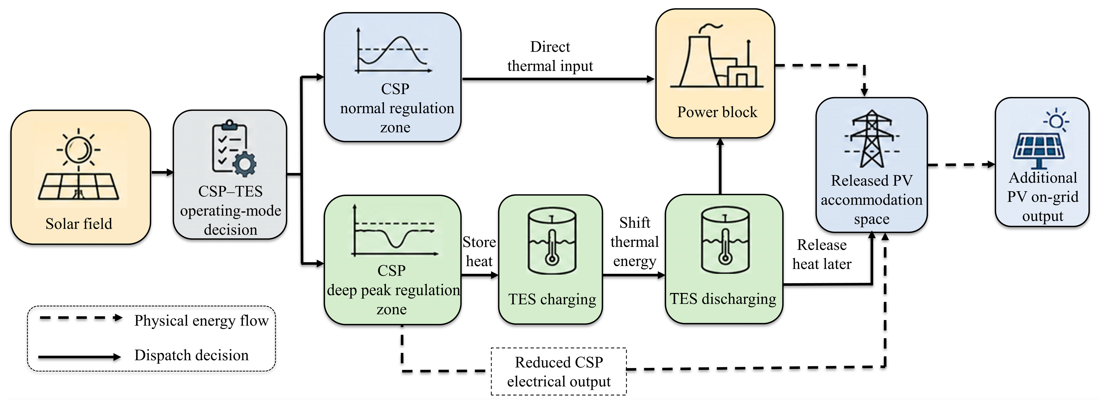
Figure 1: CSP–TES energy flow and operating boundaries under normal and deep peak regulation modes.

2.3 CCER-Based Deep Peak Regulation Dual-Compensation Mechanism

Deep peak regulation imposes additional operating burdens on CSP plants. When the electrical output of a CSP plant is reduced below its basic deep peak regulation level, the heat-to-power conversion efficiency may decrease, and additional TES-related thermal dissipation may occur. Similar efficiency-loss and compensation issues have been discussed in CSP deep peak regulation and CSP–PV hybrid dispatch studies [5,10]. Therefore, conventional ancillary-service compensation alone may be insufficient to cover the incremental operating cost of CSP deep peak regulation.

From a system perspective, CSP downward regulation can release generation space for PV during periods of high solar availability. This is consistent with the peak-shaving role of CSP in PV–CSP hybrid systems [5]. More PV electricity can then be delivered to the grid, increasing the associated carbon-emission-reduction value.

The mechanism includes two coordinated revenue channels. First, the CSP plant receives dynamic deep peak regulation compensation according to the system deep peak regulation requirement and the engineering-equivalent cost of deep peak regulation. Second, a defined share of the CCER revenue generated from actual PV on-grid electricity is allocated to the CSP plant through a dynamic sharing coefficient. The sharing process is constrained by the PV plant’s reservation utility, ensuring that the post-sharing PV revenue remains acceptable.

The proposed framework does not replace ancillary-service compensation with carbon revenue. Instead, CCER revenue sharing serves as a supplementary and conditional incentive for CSP deep peak regulation. The additional PV accommodation attributable to CSP deep peak regulation is identified later through controlled benchmark comparison dispatches, while the CCER sharing settlement itself is calculated based on actual PV on-grid electricity.

Fig. 2 illustrates the cross-market coupling logic among CSP deep peak regulation, PV accommodation, dynamic deep peak regulation compensation, and PV-side CCER revenue sharing.

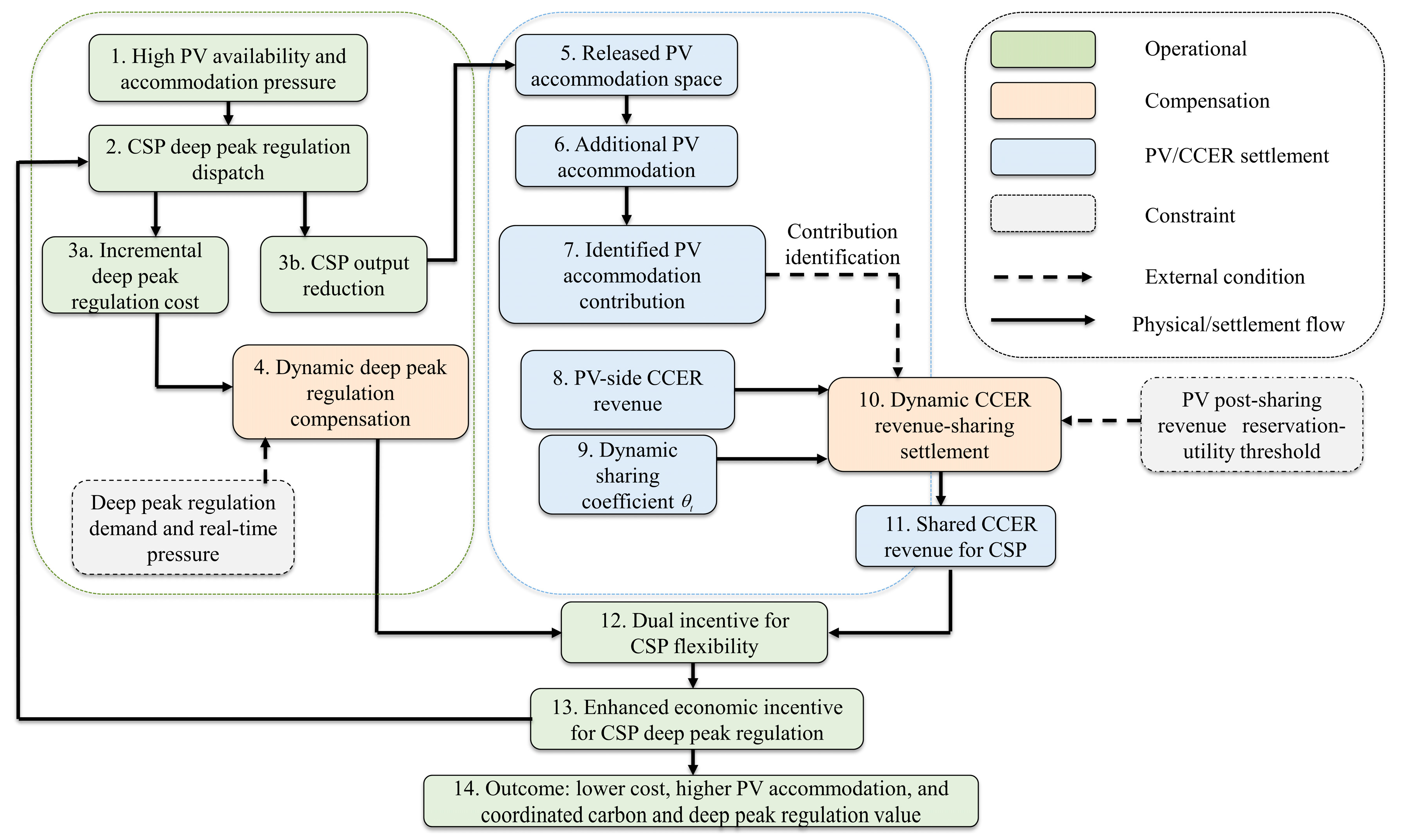
Figure 2: Cross-market dual-compensation mechanism linking CSP deep peak regulation, PV accommodation, and CCER revenue sharing.

2.3.1 Dynamic Compensation Model and Calibration Basis

Conventional fixed compensation schemes cannot fully reflect time-varying deep peak regulation requirements because compensation needs depend on regulation demand, operating state, and resource-specific cost characteristics [10]. Therefore, a dynamic compensation model is established to adjust the CSP compensation rate according to system deep peak regulation demand and real-time regulation pressure.

The compensation baseline is defined as an engineering-equivalent incremental operating cost of CSP deep peak regulation. This baseline is not intended to describe long-term lifetime degradation, mechanical fatigue, or component aging in a detailed physical sense. Instead, it monetizes two short-term operational effects that occur when the CSP plant operates below its basic deep peak regulation level: the reduction in heat-to-power conversion efficiency and the additional thermal dissipation associated with TES operation.

For each scheduling interval, the unit compensation baseline is calculated as follows:

The first term in the numerator of Eq. (1) represents the loss of electrical-output value caused by the reduction in heat-to-power conversion efficiency. The second term represents the additional thermal dissipation associated with the changed TES operating state. The denominator normalizes these incremental effects by the deep peak regulation power range in the corresponding interval, yielding the unit compensation baseline for CSP deep peak regulation.

The parameters η c s p base , η c s p deep , and η h are treated as representative operating-state parameters over the day-ahead scheduling horizon. Their values are calibrated based on the CSP deep peak regulation compensation framework in Ref. [10] and the CSP–PV hybrid operating characteristics reported in Refs. [5,6]. Therefore, the proposed formulation captures short-term efficiency-loss and TES-loss effects while avoiding an unsupported representation of cumulative mechanical fatigue, long-term degradation, or detailed thermo-mechanical aging.

The dynamic compensation multiplier is then determined by the daily deep peak regulation demand and real-time regulation pressure, as shown in Eq. (2). The final compensation rate and total CSP compensation are obtained by combining the calibrated unit baseline with this dynamic multiplier, as shown in Eq. (3). λt=(δd+δpr,t)2δ1=1T∑t=1T(Pnet,t−P_net)2/P_netδd=βδ1−δ1,minδ1,max−δ1,min+1δ2,t=Pnet,t∑i=1nPi,min−Pcsp,minδpr,t=βδ2,max−δ2,tδ2,max−δ2,min+1(2) Kcsp,t=λtctbaseCcspcomp=∑t=1TKcsp,t(Pcsp,mindeep−Pcsp,t)Δt(3) where t and i denote the indices of scheduling intervals and thermal units, respectively; T and n are the total numbers of scheduling intervals and thermal units; and Δ t is the duration of a single scheduling interval. C c s p comp denotes the total CSP deep peak regulation compensation cost, and K c s p , t is the unit capacity compensation rate at time t. P c s p , t and P c s p , min deep represent the actual CSP electrical output and the baseline minimum output under deep peak regulation, respectively.

For the physical cost parameters, p c s p denotes the benchmark on-grid price of the CSP plant. η c s p base and η c s p deep are the heat-to-power conversion efficiencies under basic and compensated deep peak regulation states, respectively. P h , t deep denotes the thermal power associated with the deep peak regulation state, η h is the thermal dissipation coefficient, and Q h , t base and Q h , t deep denote the TES energy levels under the basic and deep peak regulation states.

Furthermore, δ d and δ p r , t denote the daily deep peak regulation demand coefficient and the real-time regulation-pressure coefficient, respectively. They are derived from the system net load P net , t , its average value P _ net , and the specific demand and pressure indices δ 1 and δ 2 , t , which are bounded by their corresponding limits. P i , min and P c s p , min represent the minimum output limits of thermal unit i and the CSP plant, respectively. The coefficient β reflects the maximum compensation intensity set by the grid operator.

The numerical values and source basis of the heat-to-power efficiency and TES thermal dissipation parameters are provided in Appendix A Table A2.

2.3.2 CCER Dynamic Revenue-Sharing Model

CSP deep peak regulation can increase PV accommodation by reducing CSP electrical output during periods of high PV availability. In the proposed mechanism, the CCER revenue of the PV plant is calculated based on actual PV on-grid electricity, the regional grid carbon-emission factor, and the CCER transaction price.

Existing CCER-sharing studies have mainly examined carbon-revenue redistribution for thermal-unit deep peak regulation [20]. In contrast, this study considers a CSP–TES plant whose deep peak regulation capability is constrained by coupled thermal-energy balance and storage-state conditions. PBDR is also incorporated to coordinate load-side flexibility with source-side deep peak regulation.

A dynamic sharing coefficient is introduced to determine the proportion of PV-side CCER revenue allocated to the CSP plant. This coefficient varies with the operating condition and reflects the intensity of deep peak regulation demand and the economic requirement of CSP deep peak regulation. The PV plant’s individual-rationality constraint ensures that its post-sharing net revenue remains no lower than its reservation utility.

Fig. 3 illustrates the output-substitution and settlement logic under different CSP deep peak regulation compensation modes. Without deep peak regulation participation, PV accommodation remains limited and no additional compensation is triggered. Under the single-compensation mode, the CSP plant reduces its electrical output and receives deep peak regulation compensation. Under the proposed dual-compensation mode, CSP deep peak regulation further releases PV accommodation space, and a defined share of PV-side CCER revenue is allocated to the CSP plant as an additional conditional incentive.

As shown in Fig. 3, CCER revenue sharing serves as a supplementary incentive rather than an unconditional transfer of PV carbon revenue. The mechanism combines ancillary-service compensation with PV-side carbon-value sharing to improve the incentive for CSP deep peak regulation while preserving the economic acceptability of PV participation.

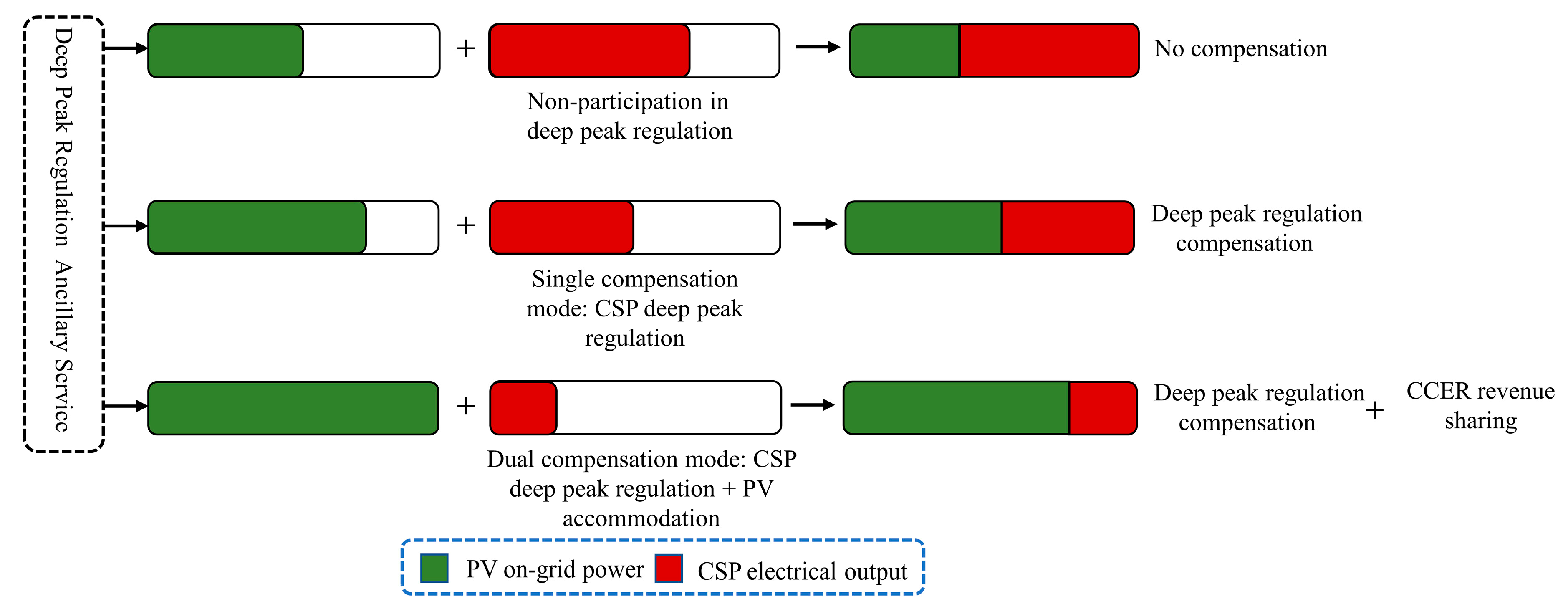
Figure 3: CSP–PV output substitution and settlement logic under different CSP deep peak regulation compensation modes.

The quantitative model is constructed as follows.

• (1)CCER revenue calculation. The CCER revenue generated by the PV station, Cv,tccer, is calculated based on actual PV on-grid output Pv,t, the regional grid carbon-emission factor ξ, and the CCER transaction price:Cv,tccer=ξPv,tpccer,tΔt(4)where pccer,t denotes the unit transaction price of CCER during period t.

• (2)Dynamic sharing mechanism. The shared CCER benefit allocated to the CSP plant, Ccspshare, is determined by introducing the dynamic sharing coefficient θt. This mechanism allocates a time-varying share of PV-side CCER revenue to the CSP plant and establishes a financial link between PV accommodation and CSP deep peak regulation:Ccspshare=∑t=1TθtCv,tccer(5)

• (3)Satisfaction coupling constraint. To satisfy the PV plant’s individual-rationality requirement, a PV satisfaction index εt is constructed as follows:0≤θt≤θmaxεt≥εminεt=1−θt/θmax−Sv−Pv,tpre/κSv(6)where εt decreases as the sharing coefficient θt increases. This constraint limits the revenue claim of the CSP plant and ensures that the PV station’s post-sharing net revenue remains above its reservation-utility threshold εmin. The parameter θmax represents the maximum allowable sharing limit. The buffer factor κ is introduced to prevent numerical singularities during periods of low or zero PV output. Finally, Pv,tpre and Sv denote the predicted PV power output and the installed PV capacity, respectively.

3 Bi-Level Optimal Dispatch Model for the CSP–PV System Based on Fuzzy Satisfaction

3.1 Fuzzy Chance-Constrained Modeling for Source-Load Uncertainty

PV available output and electrical load demand are uncertain in day-ahead scheduling. Newly commissioned renewable facilities may not provide enough historical observations for reliable probability-distribution fitting. Therefore, fuzzy chance-constrained programming is adopted to characterize epistemic uncertainty under limited samples [21,22].

In this study, only PV available output and load demand are treated as uncertain variables. The CCER price, demand-price elasticity matrix, CSP–TES operating parameters, and deep peak regulation compensation parameters are treated as deterministic inputs within each day-ahead scheduling case. To keep the uncertainty representation consistent, both PV output and load demand are described by triangular fuzzy numbers.

The membership functions of PV output and load demand are denoted by A ( P v , t ) and A ( P load , t ) , respectively. The PV available output is represented by the following triangular membership function:

Similarly, the load demand is described by:

Accordingly, PV output and load demand are represented by triangular fuzzy numbers: P˜v,t=(av,t,bv,t,cv,t)=(kv1,1,kv3)Pv,tpreP˜load,t=(aload,t,bload,t,cload,t)=(kload1,1,kload3)Pload,tpre(9) where a v , t , b v , t , c v , t denote the lower bound, most likely value, and upper bound of the triangular fuzzy number for PV output, respectively. Similarly, a load , t , b load , t , c load , t denote the corresponding membership parameters for load demand. The proportional coefficients k v 1 , k v 3 , k load 1 and k load 3 are determined from the statistical characteristics of historical prediction errors. Consequently, P ˜ v , t and P ˜ load , t represent the fuzzy variables for PV output and load demand, while P load , t pre denote their forecasted values.

This triangular fuzzy representation captures PV and load uncertainty without requiring explicit probability-distribution fitting. The resulting source–load uncertainty is incorporated into the reserve constraint in Section 3.3, where the fuzzy chance constraint is transformed into its deterministic equivalent based on fuzzy credibility theory [22].

3.2 Upper-Level Model: Net Load Smoothing via PBDR

As shown in Fig. 4, the proposed framework consists of an upper-level PBDR model, a lower-level source-side dispatch model, and two settlement channels linked to the carbon trading market and the deep peak regulation ancillary-service market. The upper-level model reshapes the load profile through PBDR, while the lower-level model optimizes the coordinated dispatch of thermal units, CSP–TES, and PV generation under system operating constraints.

In the upper level, PBDR adjusts flexible demand according to the time-of-use electricity price and the demand-price elasticity matrix. Its objective is to reduce the net-load peak-to-valley difference while maintaining total daily electricity consumption unchanged. The resulting post-PBDR load profile is then transferred to the lower-level source-side dispatch model as the load-side dispatch input.

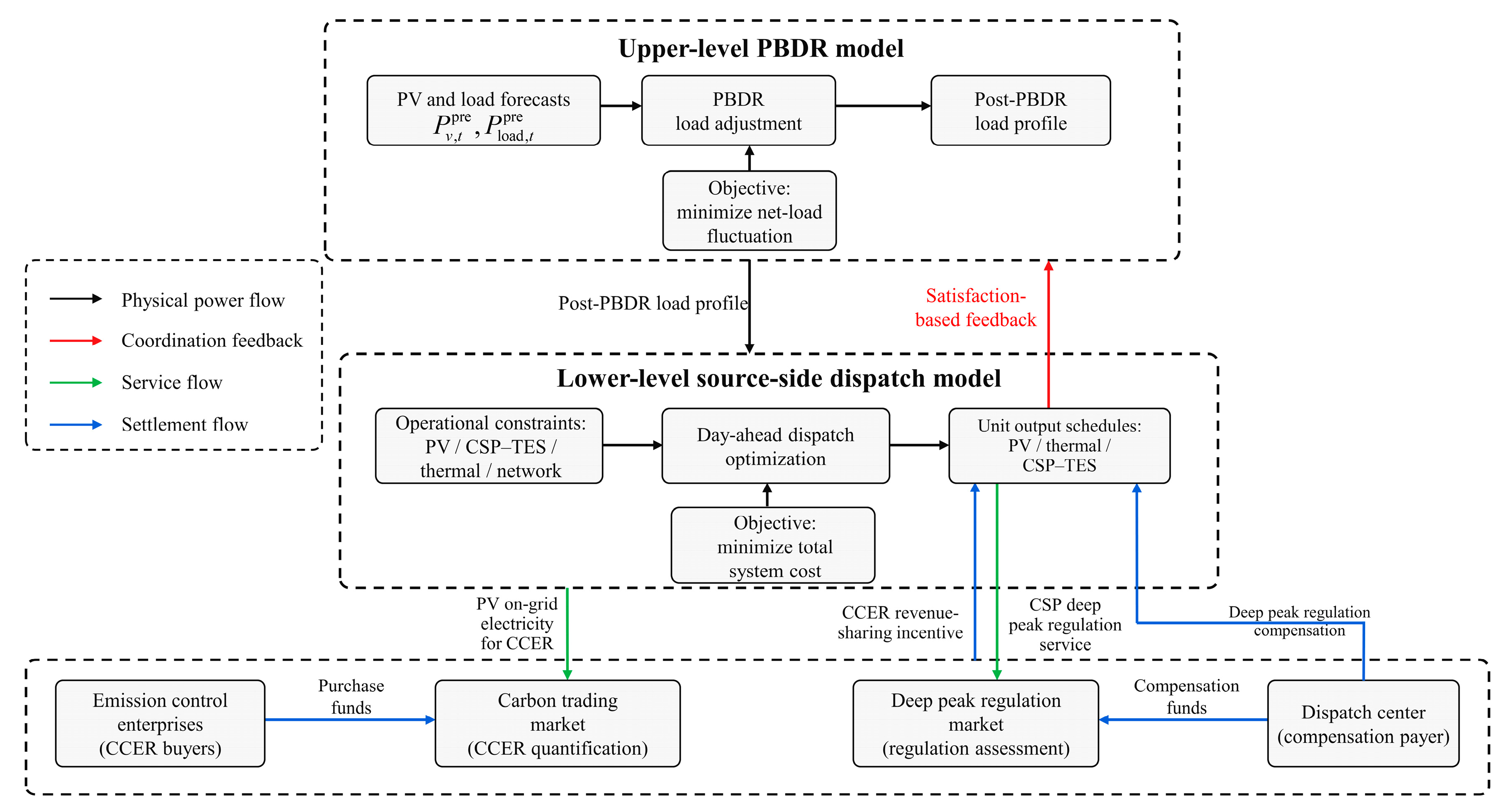
Figure 4: Overall bi-level dispatch and dual-settlement framework for the CSP–PV system.

3.2.1 Objective Function

The upper-level model smooths the net-load profile by adjusting flexible demand through PBDR. This reduces hour-to-hour net-load fluctuations and alleviates the ramping and deep peak regulation burden on the lower-level source-side dispatch model. Accordingly, the upper-level objective f 1 is formulated as follows: minf1=∑t=1T−1(Pnet,t+1−Pnet,t)2(10) Pnet,t=Pload,t1−Pv,tpre(11) where P load , t 1 is the electrical load power after PBDR at time t, and P net , t is the net load power at time t.

3.2.2 Operational Constraints

The upper-level PBDR model is subject to constraints on total electricity consumption, time-of-use price limits, and user satisfaction. These constraints ensure that the load adjustment remains physically feasible and economically acceptable for demand-side participants.

The total daily electricity consumption is kept unchanged:

The post-PBDR peak-to-valley price ratio is bounded as follows:

The electricity-consumption-mode satisfaction and electricity-cost satisfaction are constrained by: 1−∑t=1T|ΔPload,t|∑t=1TPload,t0≥Sminmode(14) 1−∑t=1T(Pload,t1Dt1−Pload,t0Dt0)∑t=1TPload,t0Dt0≥Smincost(15) where Δ P load , t denotes the change in electrical load after PBDR. D p 1 and D g 1 represent the peak-period and valley-period electricity prices after PBDR, respectively. P load , t 0 denotes the baseline electrical load before PBDR. S min mode and S min cost are the minimum satisfaction thresholds for the electricity-consumption mode and electricity cost, respectively. D t 0 and D t 1 denote the electricity prices before and after PBDR.

To link the hourly dispatch model with the time-of-use pricing mechanism, the 24-h scheduling horizon is divided into peak, flat, and valley periods, denoted by T p , T f , and T g , respectively. The hourly electricity price D t is determined by the following stepwise mapping: Dt=Dp,ift∈TpDf,ift∈TfDg,ift∈Tg(16) where D p , D f , and D g denote the electricity prices in peak, flat, and valley periods, respectively. This mapping applies to both the baseline prices D t 0 and the optimized prices D t 1 after PBDR.

The demand-response relationship is modeled using the demand price elasticity matrix. The price elasticity coefficient is defined as:

The demand price elasticity matrix is given by:

The post-PBDR load levels in peak, flat, and valley periods are then obtained as: Pload,p1Pload,f1Pload,g1=Pload,p0000Pload,f0000Pload,g0EΔDpDp0ΔDfDf0ΔDgDg0+Pload,p0Pload,f0Pload,g0(19) where Δ D t denotes the electricity price variation for PBDR, and ε P is the demand price elasticity coefficient. P load , p 0 , P load , f 0 , P load , g 0 denote the baseline loads in peak, flat, and valley periods, respectively, while P load , p 1 , P load , f 1 , P load , g 1 denote the corresponding loads after PBDR. Similarly, D p 0 , D f 0 , D g 0 represent the baseline electricity prices, while Δ D p , Δ D f , Δ D g represent the corresponding price variations. E is the demand price elasticity matrix, in which the diagonal elements represent self-elasticity coefficients and the off-diagonal elements represent cross-elasticity coefficients.

3.3 Lower-Level Model: Coordinated Multi-Source Dispatch

3.3.1 Objective Function

The lower-level model minimizes the total system operating cost C min under the post-PBDR load profile obtained from the upper-level model. The objective represents the coordinated economic dispatch of thermal units, PV generation, and the CSP–TES plant. Eq. (20) defines the total cost, which consists of thermal-unit operating cost C a , system maintenance cost C b , PV curtailment penalty C c , daily TES amortization cost C d , CSP deep peak regulation cost C c s p deep , thermal-unit deep peak regulation cost C t h deep , and net carbon trading cost C carbon .

Eq. (21) gives the thermal-unit operating cost C a , including fuel cost and start-up cost.

Eq. (22) calculates the system maintenance cost and PV curtailment penalty. The maintenance cost includes the operation and maintenance costs of the CSP and PV plants, while the curtailment penalty penalizes curtailed PV power.

Eq. (23) gives the daily TES amortization cost. It converts the capacity and power investment costs of the TES system into an equivalent daily cost through the capital recovery factor.

Eq. (24) describes the deep peak regulation costs of thermal units and the CSP plant. For thermal units, the cost is represented by an oil-consumption loss coefficient when the unit output falls below its critical deep peak regulation level. For the CSP plant, the cost follows the engineering-equivalent compensation baseline defined in Section 2.3.1, which captures short-term heat-to-power efficiency loss and TES-related thermal dissipation.

Eq. (25) calculates the net carbon trading cost by comparing total thermal-unit carbon emissions with the freely allocated carbon-emission quota. Ccarbon=pco2∑t=1T∑i=1nμiPi,tΔt−Qquota(25) where e 1 and e 2 denote the fuel cost and start-up cost of thermal units, respectively. P i , t is the power output of thermal unit i at time t, and a i , b i , and c i are its fuel-cost coefficients. s i denotes the single start-up cost, and U i , t is a binary variable indicating the on/off status of thermal unit i.

For renewable and CSP-related cost terms, s c s p and s v denote the operation and maintenance cost coefficients of the CSP and PV plants, respectively. k v is the penalty coefficient for PV curtailment, and P v , t curt denotes the curtailed PV power at time t.

For the TES system, C h denotes the unit initial investment cost, r is the discount rate, and Y is the service life of the TES system. C inv represents the total capacity and power investment cost, E h , max is the maximum thermal storage capacity, C c s p , p is the unit power investment cost of the CSP plant, and P h , max out denotes the maximum heat-release power. C h om and s h denote the TES operation and maintenance cost and its corresponding coefficient.

For deep peak regulation and carbon-cost terms, γ i denotes the oil-consumption loss coefficient of thermal unit i, and P i deep is the critical output threshold for thermal-unit deep peak regulation. μ i denotes the carbon-emission factor of thermal unit i, p co 2 is the baseline carbon trading price, and Q quota represents the freely allocated carbon-emission quota.

3.3.2 Operational Constraints

• (1)Active-power balance and thermal-unit operating constraints.

At the system level, the aggregate active-power balance is imposed in each scheduling interval to ensure that the total generation from PV, CSP, and thermal units meets the post-PBDR load demand:

Thermal units are further constrained by minimum up/down time requirements, ramping limits, and output bounds: ∑k=tmin(t+Ti,minon−1,T)Ui,k≥Ti,minon(Ui,t−Ui,t−1)∑k=tmin(t+Ti,minoff−1,T)(1−Ui,k)≥Ti,minoff(Ui,t−1−Ui,t)(27) Pi,t−Pi,t−1≤Ui,t−1RiuΔt+(Ui,t−Ui,t−1)Pi,maxPi,t−1−Pi,t≤Ui,tRidΔt−(Ui,t−Ui,t−1)Pi,min(28) Ui,tPi,min≤Pi,t≤Ui,tPi,max(29) where T i , min on/off denote the minimum up and down time requirements of thermal unit i, respectively. R i u/d represent the ramp-up and ramp-down limits. P i , max and P i , min denote the maximum and minimum output limits of thermal unit i. U i , t is the binary on/off status of thermal unit i at time t.

• (2)CSP–TES energy-flow and operating constraints.

The CSP–TES plant is modeled through the coupling of solar-thermal collection, direct thermal input to the power block, TES charging, TES discharging, and electrical power generation. The collected solar-thermal power P c s p , t S , H , TES charging power P h , t in , TES discharging power P h , t out , and direct thermal input to the power block P c s p , t H , RC satisfy the following energy-flow balance:

TES charging and discharging powers are limited by their capacity bounds and binary operating states. Simultaneous charging and discharging are not allowed:

The TES energy balance, storage-capacity limits, and initial/final storage-state requirements are given by:

The CSP electrical output is constrained by its unit commitment status and output limits:

The minimum up/down time and ramping constraints of the CSP plant are expressed as: ∑k=tmin(t+Tcsp,minoff−1,T)(1−Ucsp,k)≥Tcsp,minoff(Ucsp,t−1−Ucsp,t)∑k=tmin(t+Tcsp,minon−1,T)Ucsp,k≥Tcsp,minon(Ucsp,t−Ucsp,t−1)(34) Pcsp,t−Pcsp,t−1≤Ucsp,t−1RcspuΔt+(Ucsp,t−Ucsp,t−1)Pcsp,maxPcsp,t−1−Pcsp,t≤Ucsp,tRcspdΔt−(Ucsp,t−Ucsp,t−1)Pcsp,min(35) where η h in and η h out denote the TES charging and discharging efficiencies, respectively. U h , t in and U h , t out are binary variables indicating the charging and discharging states of the TES system. P h , max in and P h , max out are the maximum charging and discharging power limits. E h , t denotes the TES energy level at time t, while E h , 1 and E h , T denote the initial and final TES energy levels. E h , min and E h , max are the minimum and maximum thermal storage limits. η h 1 and η h 2 are the lower and upper coefficients for the final-to-initial TES energy ratio. U c s p , t is the binary operating status of the CSP plant, and [ P c s p , min , P c s p , max ] defines its output range. T c s p , min on/off denote the minimum up/down time requirements of the CSP plant, and R c s p u/d denote its ramp-up and ramp-down limits.

• (3)PV and CCER settlement constraint.

The PV on-grid output is limited by the available PV output forecast, and curtailed PV power is defined as the difference between available PV output and actual on-grid PV output:

To support the economic viability of CSP deep peak regulation, the combined compensation received by the CSP plant should cover its deep peak regulation operating cost:

The PV plant’s individual-rationality constraint is introduced to ensure that its net revenue under coordinated dispatch is no lower than that under standalone operation: Rv=∑t=1T(pv−sv)Pv,tΔt+(1−θt)Cv,tccer−kvPv,tcurtΔtRvbase=∑t=1T(pv−sv)Pv,tbaseΔt+Cv,tccer,base−kvPv,tcurt,baseΔtCv,tccer,base=ξpccer,tPv,tbaseΔtRv≥Rvbase(39) where R v and R v base denote the PV plant’s net revenue under coordinated dispatch and standalone operation, respectively. p v is the PV electricity selling price, and s v is the PV operation and maintenance cost coefficient. Under coordinated dispatch, P v , t and P v , t curt denote the PV on-grid output and curtailed PV power at time t, respectively. Under standalone operation, P v , t base and P v , t curt , base denote the corresponding on-grid output and curtailed PV power. C v , t ccer , b a s e denotes the CCER revenue generated from the standalone PV on-grid output. The sharing coefficient θ t determines the share of PV-side CCER revenue allocated to the CSP plant. This constraint preserves the economic acceptability of PV participation in the coordinated dispatch mechanism.

• (4)DC power-flow and transmission constraints.

Eq. (26) gives the aggregate active-power balance of the system. To further represent network feasibility, the post-PBDR load is allocated to individual buses according to the baseline nodal-load proportion. The active load at bus b during period t is expressed as: Pload,b,t1=ωbPload,t1ωb=Db0∑k∈NDk0，∀b∈N，∀t(40) where D b 0 is the baseline active load at bus b, ω b is the corresponding nodal-load proportion, and N denotes the set of buses. This formulation preserves the original nodal-load distribution while allowing the total load level to be adjusted by PBDR.

For each bus, the nodal active-power balance is enforced as follows: ∑i∈GbPi,t+Pcsp,b,t+Pv,b,t−Pload,b,t1=∑j∈NbFbj,t，∀b∈N，∀t(41) where G b denotes the set of thermal units connected to bus b , N b is the set of buses directly connected to bus b , and F b j , t is the active-power flow from bus b to bus j . In the modified IEEE 30-bus system, the CSP plant and PV plant are connected to their designated buses, while the corresponding injections at the remaining buses are set to zero.

Under the DC power-flow approximation, the active-power flow on branch ( b , j ) is determined by the voltage-angle difference: Fbj,t=δb,t−δj,txbj，∀(b,j)∈L，∀t−F¯bj≤Fbj,t≤F¯bj，∀(b,j)∈L，∀tδb0,t=0，∀t(42) where x b j and F ¯ b j denote the reactance and transmission capacity of branch ( b , j ) , respectively; δ b , t is the voltage phase angle at bus b ; L is the set of transmission branches; and b 0 denotes the reference bus. Eqs. (40)–(42) ensure that the dispatch decisions satisfy nodal active-power balance and branch transmission limits.

The DC network model is adopted for day-ahead active-power scheduling and comparative mechanism evaluation. It represents nodal active-power balance and transmission-flow limits, but it does not include voltage magnitudes, reactive-power dispatch, PV inverter reactive-power capability, or static reactive compensation as decision variables. Therefore, the numerical results should be interpreted as active-power dispatch results under the DC approximation rather than as a local voltage-stability assessment.

Since all benchmark scenarios are evaluated under the same nodal network representation and branch transmission limits, the comparative results reflect the relative effects of PBDR, deep peak regulation compensation, CCER revenue sharing, and uncertainty treatment within a consistent day-ahead dispatch framework.

• (5)System spinning reserve with fuzzy chance constraints.

Based on the triangular fuzzy representations introduced in Section 3.1, the uncertain net load at time t is expressed as: W˜t=P˜load,t−P˜v,t=(w1,t,w2,t,w3,t)(43) w1,t=aload,t−cv,tw2,t=bload,t−bv,tw3,t=cload,t−av,t(44) where w 1 , t , w 2 , t and w 3 , t represent the lower bound, most likely value, and upper bound of the triangular fuzzy net load, respectively. Therefore, the uncertainty of PV available output and load demand is jointly reflected in the spinning-reserve requirement.

Let G t u p denote the maximum available system supply at time t after upward reserve deployment, excluding the uncertain PV output:

For a triangular fuzzy number W ˜ t = w 1 , t , w 2 , t , w 3 , t , the credibility distribution of the event W ˜ t ≤ x is:

To ensure that the available generation capacity can satisfy the uncertain net load at the prescribed confidence level α , the fuzzy chance constraint is formulated as: CrGtup≥W˜t≥αGtup≥w2,t+(2α−1)w3,t−w2,t，α∈[0.5,1].(47) where C r { ⋅ } denotes the credibility measure. Since the credibility level adopted in the case study is higher than 0.5, the deterministic equivalent is obtained from the right-hand branch of the triangular fuzzy credibility distribution. The resulting constraint requires the available upward reserve capacity to cover a confidence-adjusted net-load level located between the most likely value w 2 , t and the upper bound w 3 , t .

Because w 2 , t , w 3 , t , and α are known before optimization, Eq. (47) is a linear deterministic constraint and can be directly incorporated into the lower-level MILP model. A larger credibility level increases the required reserve margin and improves operational robustness, while also increasing the conservatism of the dispatch decision [22].

3.4 Fuzzy-Satisfaction-Based Bi-Level Interactive Solution Procedure

To avoid the computational burden of a full Karush–Kuhn–Tucker (KKT)-based single-level reformulation, this study adopts an iterative fuzzy-satisfaction-based solution procedure. The upper-level model first determines the post-PBDR load profile, which is then passed to the lower-level source-side dispatch model. Given this load-side input, the lower-level problem is formulated as a MILP because it includes discrete unit-commitment and operating-state variables.

The model was implemented in MATLAB 2021a with YALMIP and solved using IBM ILOG CPLEX 12.9. The relative MIP gap for each lower-level MILP was set to 10−4. Hardware specifications, model size, and runtime are reported in Section 4.1. The solution procedure is shown in Fig. 5.

To obtain a compromise solution between the system-cost objective and the CSP-revenue objective, two fuzzy satisfaction indices are constructed based on fuzzy multi-objective programming [25].

The comprehensive satisfaction metric is calculated by: A=1N∑j=1NAj(50) where A e and A c denote the satisfaction indices for the system operation cost and the CSP deep peak regulation revenue, respectively. A represents the comprehensive satisfaction metric, and A j is the satisfaction index of the j -th optimization objective. C m and C q denote the actual values of the system-cost objective and the CSP-revenue objective, respectively. Their corresponding upper and lower bounds, C m , max , C m , min , C q , max , and C q , min , are obtained from the single-objective optimization results used to construct the payoff table.

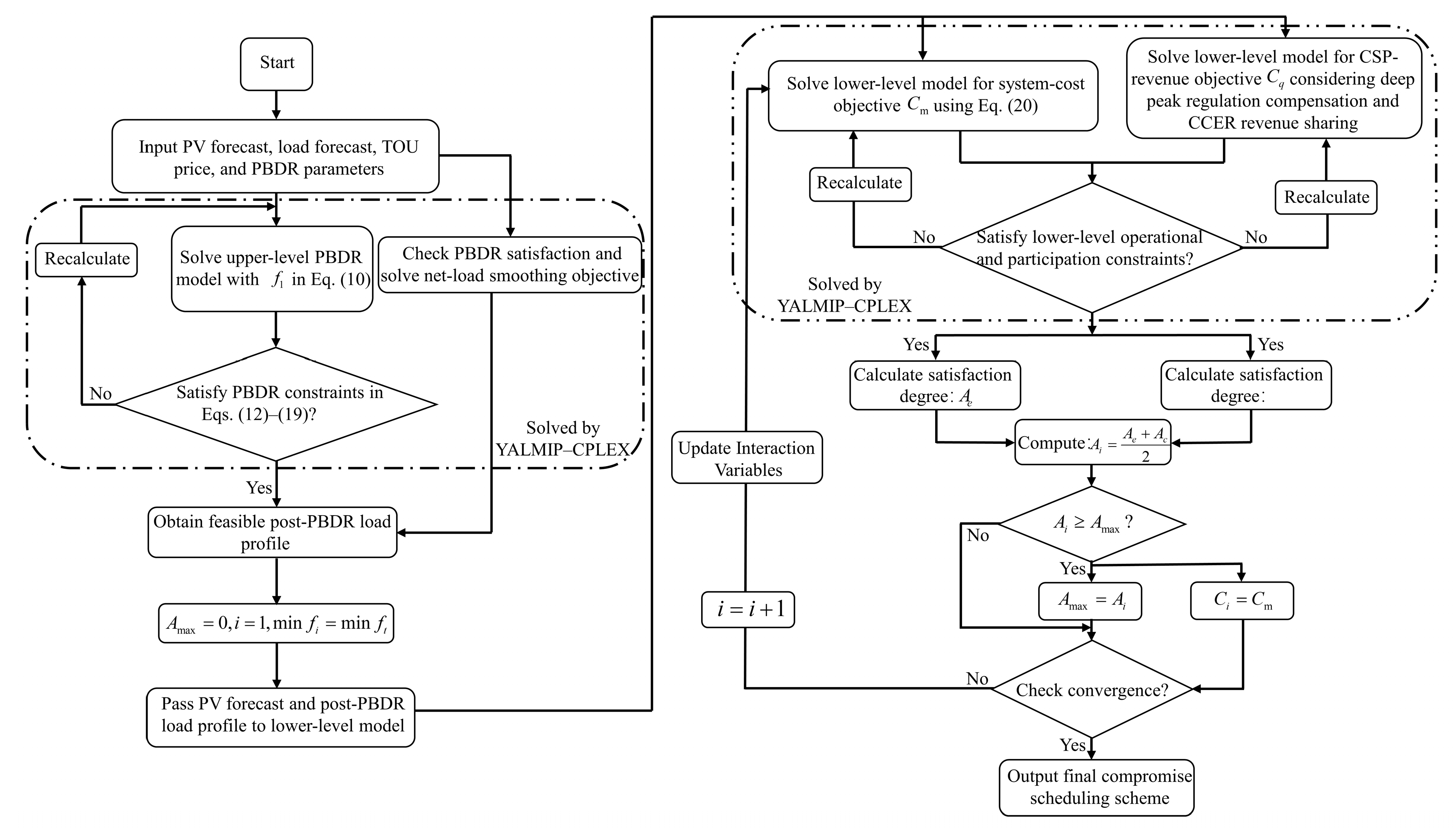
Figure 5: Solution procedure of the fuzzy-satisfaction-based bi-level interactive algorithm.

The solution steps are summarized as follows.

Step 1: Upper-Level Optimization.

The upper-level PBDR model is solved to obtain the post-PBDR load profile P l o a d , t 1 and the corresponding net-load fluctuation objective value. These results are passed to the lower-level model as load-side input parameters.

Step 2: Payoff Table Construction.

To define the ranges of the fuzzy satisfaction functions, the lower-level model is solved under single-objective settings. This process yields the boundary values C m , max , C m , min , C q , max , and C q , min , which are required for the satisfaction calculation.

Step 3: Lower-Level Dispatch optimization.

Considering the operational constraints and participation constraints, the lower-level model determines the unit output schedules and the dynamic CCER sharing coefficient θ t . This step coordinates the system operating cost with the CSP plant’s compensation and shared CCER revenue.

Step 4: Satisfaction evaluation and convergence check.

The satisfaction indices A e and A c are calculated, and the comprehensive satisfaction metric A is updated according to Eq. (50). If the convergence criterion is satisfied, the solution with the maximum comprehensive satisfaction is selected as the final compromise scheduling scheme. Otherwise, the interaction variables are updated, and the procedure returns to Step 3.

4 Case Study

4.1 Simulation Setup and Parameters

Numerical simulations are conducted on a modified IEEE 30-bus test system to evaluate the proposed dispatch mechanism with PBDR coordination and CCER-based deep peak regulation incentives [26]. As shown in Fig. 6, the conventional generator at Bus 11 is replaced with a 100 MW CSP plant, and a 200 MW PV plant is connected at Bus 13. The remaining four thermal units are retained. The day-ahead forecast profiles of load, available PV output, and available CSP thermal power are shown in Fig. 7.

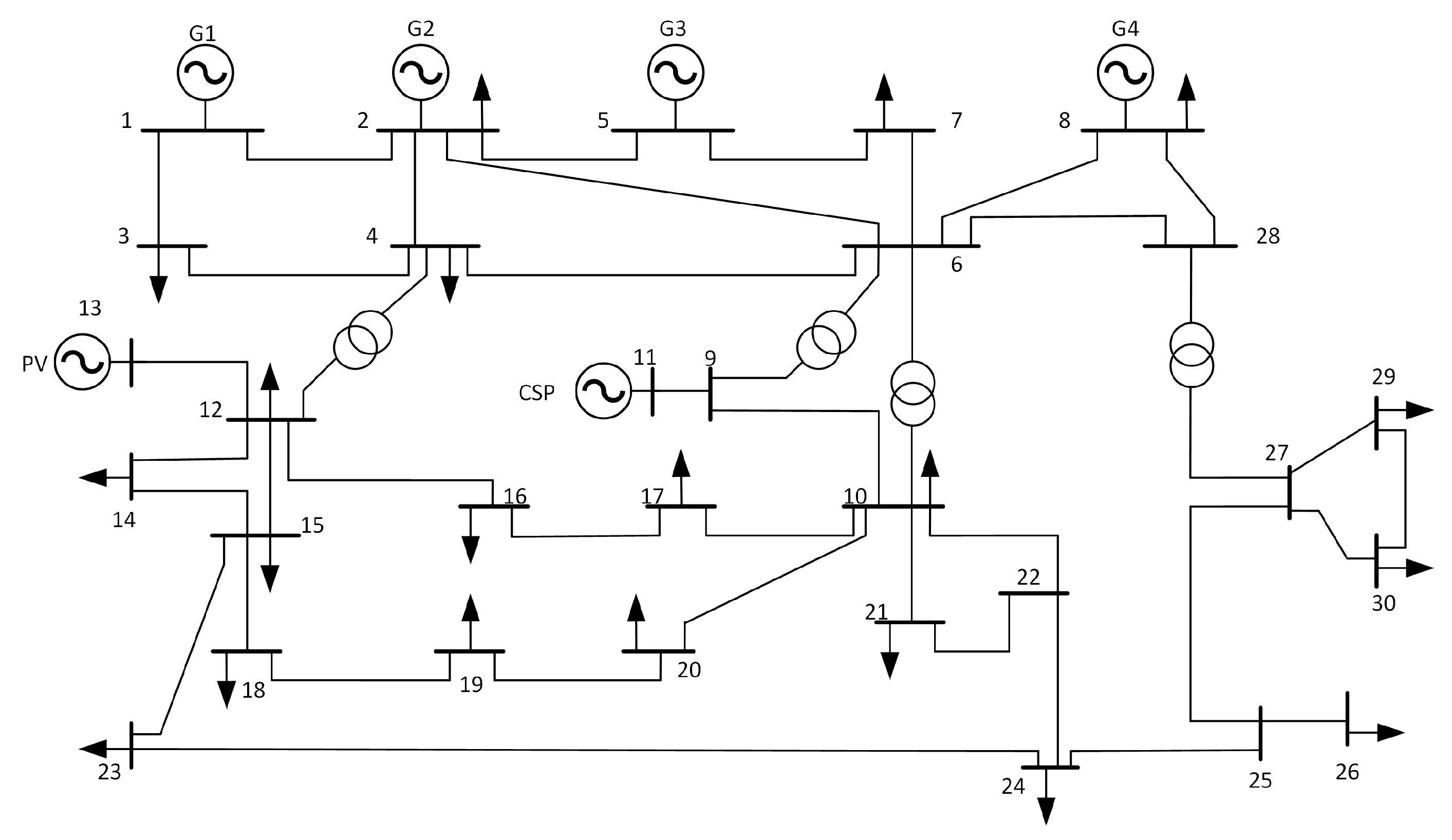
Figure 6: Modified IEEE 30-bus system after CSP and PV integration.

Consistent with the uncertainty model in Section 3.1, available PV output and load demand are represented by triangular fuzzy numbers. The corresponding fuzzy chance constraints are incorporated into the spinning-reserve requirement through the credibility-based deterministic reformulation in Section 3.3. The credibility level is set to α = 0.95 . The CCER transaction price p ccer , t is set to 50 CNY/tCO2, and the PV feed-in tariff is 300 CNY/MWh. The main technical and economic parameters are listed in Appendix A Table A1, Table A2 and Table A3. The calibration basis for the CSP heat-to-power efficiency and TES thermal dissipation parameters is provided in Appendix A Table A2.

The case study is designed to verify the internal economic logic and operational coordination effect of the proposed mechanism under a representative high-PV day-ahead scheduling condition. The modified IEEE 30-bus system provides a transparent network-constrained test environment in which the effects of PBDR, deep peak regulation compensation, CCER revenue sharing, and CSP deep peak regulation can be compared through controlled scenarios.

All simulations were carried out on a desktop computer with an Intel Core i7-10700 processor at 2.90 GHz, 16 GB of RAM, and a 64-bit Windows 10 operating system. The model was implemented in MATLAB 2021a with YALMIP and solved using IBM ILOG CPLEX 12.9. For the 24-h Scenario 5 case, the largest lower-level MILP contained approximately 400 binary variables and 2300 continuous variables. These variables mainly describe thermal-unit commitment, CSP–TES operating states, generation and reserve schedules, CCER settlement, and DC network constraints. The upper-level PBDR problem is continuous and is solved separately within the bi-level solution procedure. The procedure converged after 12 iterations and required approximately 58 s in total. The relative MIP gap for each lower-level MILP and the convergence tolerance of the bi-level solution procedure were both set to 10−4.

The simulations should not be interpreted as full engineering validation across multiple operating days, large-scale networks, or actual CCER market-price trajectories. The time-varying CCER price profiles in Section 4.6.3 are used as sensitivity and stress-test inputs to examine the settlement response of the mechanism. Multi-day validation, larger network tests, and real-market data are left for future work.

Modern PV simulation tools, such as pvlib-python, can provide reproducible PV output modeling under different irradiance and system-configuration conditions [27]. In this paper, available PV output is treated as an exogenous day-ahead forecast because the focus is on the dispatch and settlement mechanism rather than on the PV forecasting model itself.

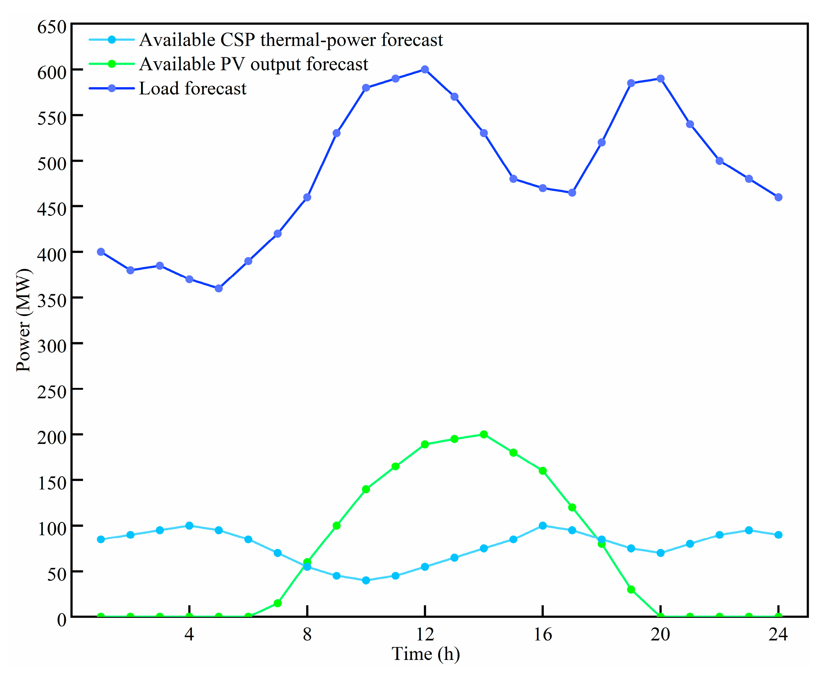
Figure 7: Day-ahead forecast profiles of load, available PV output, and available CSP thermal power.

4.2 Effect of PBDR on Net-Load Characteristics

The TOU electricity prices used for PBDR are listed in Table 3. Based on these prices and the demand price elasticity matrix, the upper-level model reshapes the load profile while keeping total daily electricity consumption unchanged.

As shown in Fig. 8, PBDR shifts part of the flexible demand from the original peak-load periods to lower-price periods. The total daily electricity consumption remains 11,655 MWh before and after PBDR, indicating that the response is achieved through temporal load shifting rather than load curtailment.

After PBDR, the load peak-to-valley difference decreases from 240 MW to 180 MW. The net-load peak-to-valley difference decreases from 387.5 MW to 293 MW, and the maximum absolute net-load ramp decreases from 160 MW/h to 138 MW/h. These results indicate that PBDR provides a smoother load-side input for the lower-level source-side dispatch model.

It should be noted that PBDR only improves the load-side operating condition. It does not directly represent the physical contribution of CSP deep peak regulation to PV accommodation. The independent and coordinated effects of PBDR, deep peak regulation compensation, and CCER revenue sharing are further examined in Section 4.3.2 and Section 4.3.3.

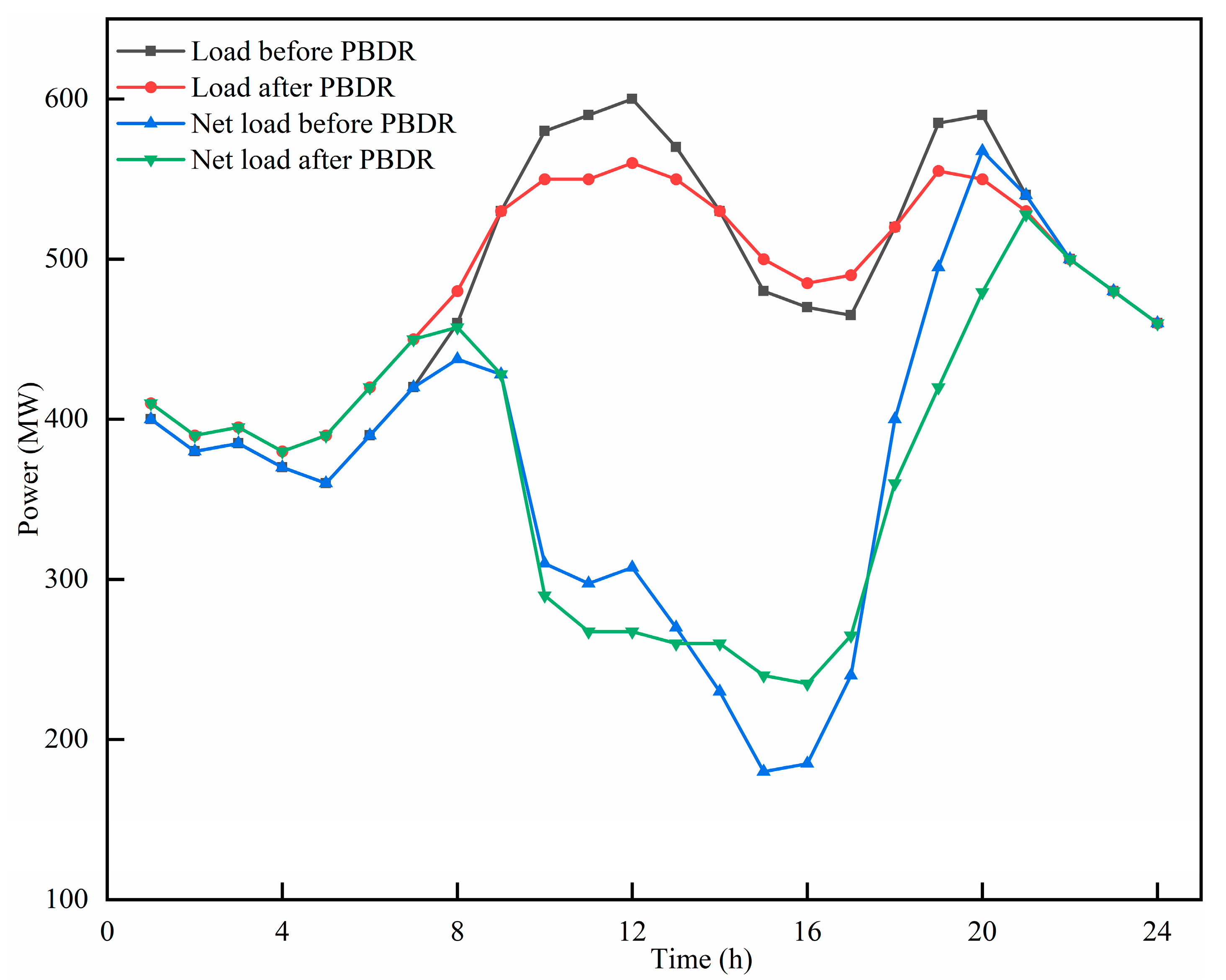
Figure 8: Load and net-load profiles before and after PBDR.

4.3 Ablation Analysis of Incentive Mechanisms and PBDR

A six-scenario ablation analysis is conducted to distinguish the independent and coordinated effects of PBDR, deep peak regulation compensation, and CCER revenue sharing. Scenarios 1–4 isolate the two source-side incentive channels. Scenario 6 evaluates the independent load-shaping effect of PBDR without source-side incentives. Scenario 5 represents the complete mechanism, in which PBDR, deep peak regulation compensation, and CCER revenue sharing are activated simultaneously. The scenario design is summarized in Table 4, and the corresponding economic results are reported in Table 5.

Compared with Scenario 1, Scenario 2 reduces the system cost by CNY 793,200, indicating that deep peak regulation compensation improves the dispatch incentive for CSP flexibility. Scenario 3 reduces the system cost by CNY 592,500 and allocates CNY 54,800 of shared CCER revenue to the CSP plant, showing the independent incentive effect of CCER revenue sharing. However, the CCER-only scenario mainly changes the settlement structure rather than directly creating sufficient physical flexibility for PV accommodation. Without explicit deep peak regulation compensation or PBDR coordination, the CSP plant still lacks adequate incentive and operating support to release additional PV accommodation space. Therefore, although Scenario 3 improves the economic allocation of dispatch benefits, its total PV-side CCER revenue is lower than that in Scenario 1, and CCER revenue sharing alone cannot independently guarantee higher PV accommodation.

Scenario 4 further reduces the system cost to CNY 1.2613 million, confirming the joint effect of the two source-side incentive channels. When PBDR is additionally activated in Scenario 5, the system cost decreases to CNY 1.2359 million, showing that load-side coordination provides an additional benefit under the dual-incentive mechanism. Scenario 6 only slightly reduces the system cost relative to Scenario 1, confirming that PBDR alone improves load-side operating conditions but cannot replace source-side incentive mechanisms.

4.3.1 Isolated and Coordinated Effects of Source-Side Incentive Mechanisms

The economic results of Scenarios 1–4 are reported in Table 5, and the corresponding dispatch profiles are shown in Fig. 9. These scenarios isolate the effects of deep peak regulation compensation and CCER revenue sharing, and then examine their coordinated effect under the dual-incentive mechanism.

In Scenario 1 [Fig. 9a], neither deep peak regulation compensation nor CCER revenue sharing is activated. The CSP plant follows its conventional operating strategy and has no additional economic incentive to provide deep downward regulation during high-PV periods. Although PV generation still creates PV-side CCER revenue, no share of this revenue is allocated to the CSP plant. As a result, the system operating cost reaches CNY 2.1077 million, the highest among Scenarios 1–4. This scenario is used as the source-side baseline.

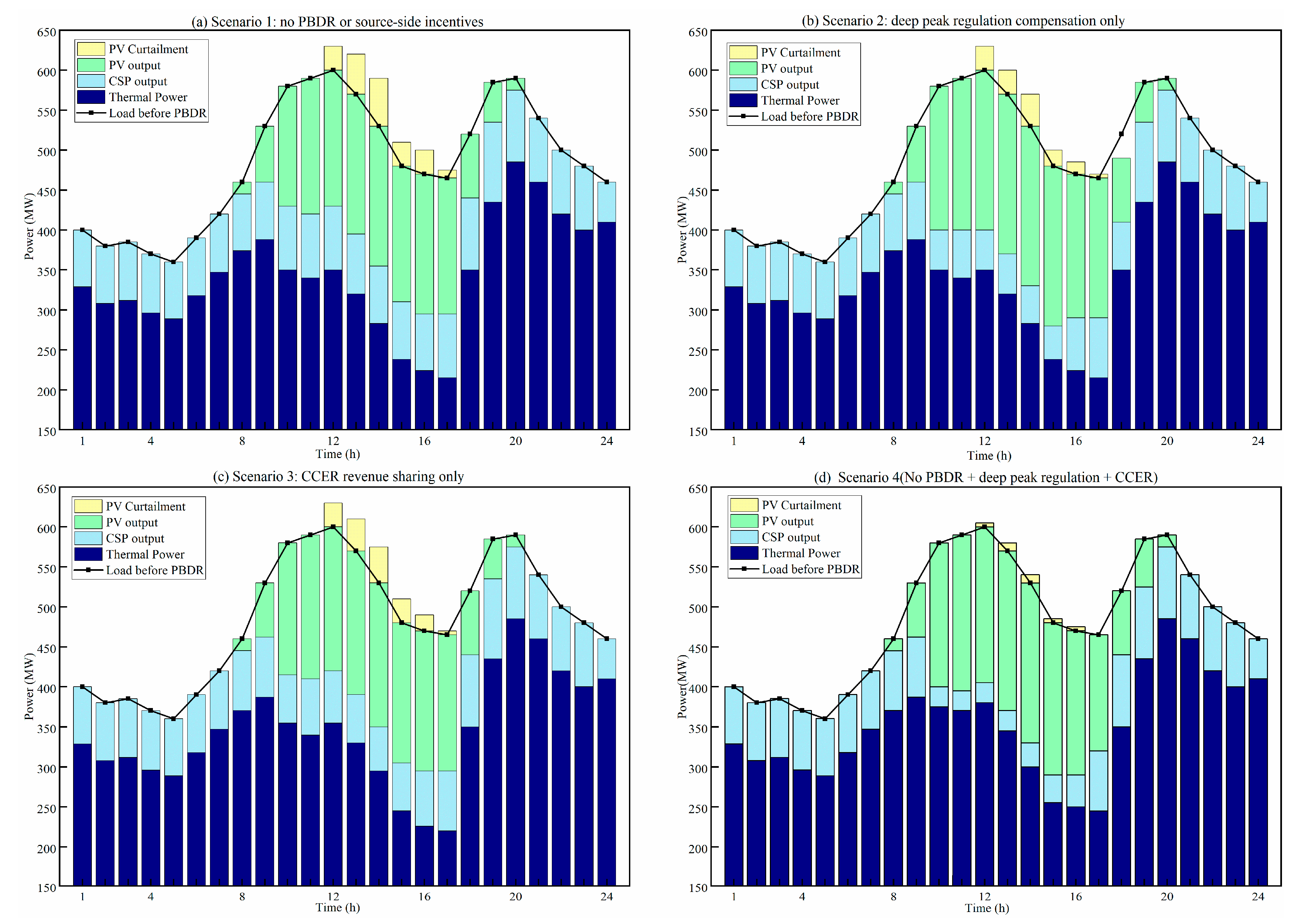
Figure 9: Dispatch profiles under source-side ablation scenarios: (a) no source-side incentives; (b) deep peak regulation compensation only; (c) CCER revenue sharing only; and (d) coordinated source-side incentives.

In Scenario 2 [Fig. 9b], only deep peak regulation compensation is activated. The CSP plant receives direct compensation for participating in deep peak regulation, and the system operating cost decreases to CNY 1.3145 million, a reduction of about 37.6% compared with Scenario 1. The CSP deep peak regulation compensation is CNY 92,900. This result shows that ancillary-service compensation can encourage CSP downward regulation and reduce the system operating cost. However, the mechanism still relies on a single compensation channel and does not transfer PV-side carbon value to the CSP plant.

In Scenario 3 [Fig. 9c], only CCER revenue sharing is activated. The CSP plant receives CNY 54,800 in shared CCER revenue, and the system operating cost decreases to CNY 1.5152 million. This cost is CNY 592,500 lower than that in Scenario 1, but CNY 200,700 higher than that in Scenario 2. Therefore, CCER revenue sharing provides an additional economic signal for CSP participation, but it cannot fully replace direct deep peak regulation compensation in covering the incremental operating cost of deep peak regulation.

In Scenario 4 [Fig. 9d], deep peak regulation compensation and CCER revenue sharing are jointly activated. The system operating cost further decreases to CNY 1.2613 million, which is CNY 53,200 lower than Scenario 2 and CNY 253,900 lower than Scenario 3. Under this coordinated setting, the CSP plant receives CNY 77,100 in deep peak regulation compensation and CNY 47,300 in shared CCER revenue. The two channels play complementary roles: deep peak regulation compensation offsets the engineering-equivalent cost of CSP deep peak regulation, while CCER revenue sharing provides an additional incentive linked to PV-side carbon value.

Overall, Scenarios 1–4 show that neither deep peak regulation compensation nor CCER revenue sharing alone can fully exploit the flexibility value of CSP–TES. Their coordinated application provides a stronger economic signal for CSP deep peak regulation and achieves the lowest system operating cost among the four source-side incentive settings.

4.3.2 Independent and Coordinated Effects of PBDR

To distinguish the independent effect of PBDR from its coordinated effect under the dual-incentive mechanism, Scenario 6 is introduced as a PBDR-only case. In Scenario 6, PBDR is activated, while CSP deep peak regulation compensation, and CCER revenue sharing are disabled. The comparison with Scenario 1 is reported in Table 6.

Compared with Scenario 1, Scenario 6 keeps the daily electricity consumption unchanged at 11,655 MWh. The load peak-to-valley difference decreases from 240 MW to 180 MW, the net-load peak-to-valley difference decreases from 387.5 MW to 293.0 MW, and the maximum absolute net-load ramp decreases from 160 MW/h to 138 MW/h. These results confirm that the primary independent role of PBDR is to reshape the load profile and reduce short-term net-load fluctuation.

The system operating cost decreases from CNY 2.1077 million in Scenario 1 to CNY 2.0631 million in Scenario 6, corresponding to a reduction of CNY 44,600. This reduction is achieved without activating CSP deep peak regulation or either of the two source-side incentive mechanisms.

However, PBDR alone does not improve PV accommodation in this case. PV on-grid energy decreases slightly from 1553 MWh to 1548 MWh, while PV curtailment increases from 205 MWh to 210 MWh. This is consistent with the upper-level PBDR objective, which minimizes net-load fluctuation rather than directly maximizing PV accommodation. Therefore, PBDR should not be interpreted as an independent PV-curtailment reduction mechanism.

As shown in Fig. 10, when PBDR is coordinated with deep peak regulation compensation and CCER revenue sharing, its role extends from load-side smoothing to improving the operating condition for source-side flexibility. Compared with Scenario 4, Scenario 5 further reduces the system operating cost from CNY 1.2613 million to CNY 1.2359 million, giving an additional reduction of CNY 25,400. The CSP deep peak regulation energy increases from 145 MWh to 185 MWh. As further quantified by the benchmark comparison dispatches in Section 4.3.3, the PV accommodation attributable to CSP deep peak regulation also increases from 145 MWh to 185 MWh.

Therefore, PBDR has two distinct roles. Independently, it smooths the load and net-load profiles and slightly reduces the system operating cost. In coordination with the dual-incentive mechanism, it improves the operating condition for CSP flexibility and allows CSP deep peak regulation to release an additional 40 MWh of PV accommodation space. This coordinated effect should not be interpreted as the independent PV-accommodation contribution of PBDR.

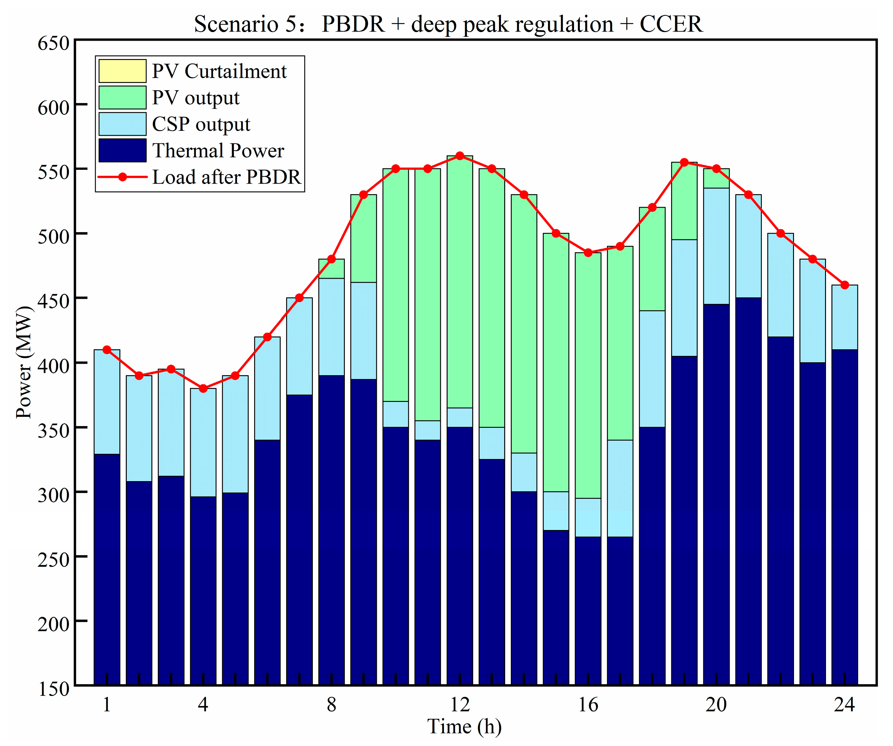
Figure 10: Dispatch profile under the complete coordinated mechanism with PBDR, deep peak regulation compensation, and CCER revenue sharing.

4.3.3 Contribution Identification of CSP Deep Peak Regulation Using Controlled Benchmark Dispatches

Although Section 4.3.1 and Section 4.3.2 quantify the economic effects of the incentive mechanisms, they do not directly identify the physical contribution of CSP deep peak regulation to PV accommodation. Therefore, controlled benchmark comparison dispatches (BCDs) are constructed for Scenarios 4 and 5. In each BCD case, the load profile, PV forecast, reserve requirement, network constraints, and settlement parameters are kept the same as those in the corresponding original scenario, while CSP deep peak regulation is disabled. The BCD cases are used only for attribution analysis and are not treated as additional independent market-clearing scenarios. Thus, Scenario 4-BCD should not be interpreted as Scenario 1, and Scenario 5-BCD should not be interpreted as Scenario 6.

Table 7 reports the BCD comparison results, and Fig. 11 further illustrates the corresponding dispatch differences during CSP deep peak regulation intervals. The added available-PV-energy row confirms that each original scenario and its corresponding BCD case are compared under the same PV availability boundary. In Scenario 4, both the original case and Scenario 4-BCD have 1758 MWh of available PV energy. When CSP deep peak regulation is disabled, PV on-grid energy decreases from 1723 MWh to 1578 MWh, while PV curtailment increases from 35 MWh to 180 MWh. Therefore, the 145 MWh difference in PV on-grid energy can be attributed to CSP deep peak regulation under the same load profile, PV forecast, reserve requirement, network constraints, and settlement settings. With CSP deep peak regulation enabled, total PV-side CCER revenue increases by CNY 15,000, and the system operating cost decreases by CNY 272,700 relative to Scenario 4-BCD.

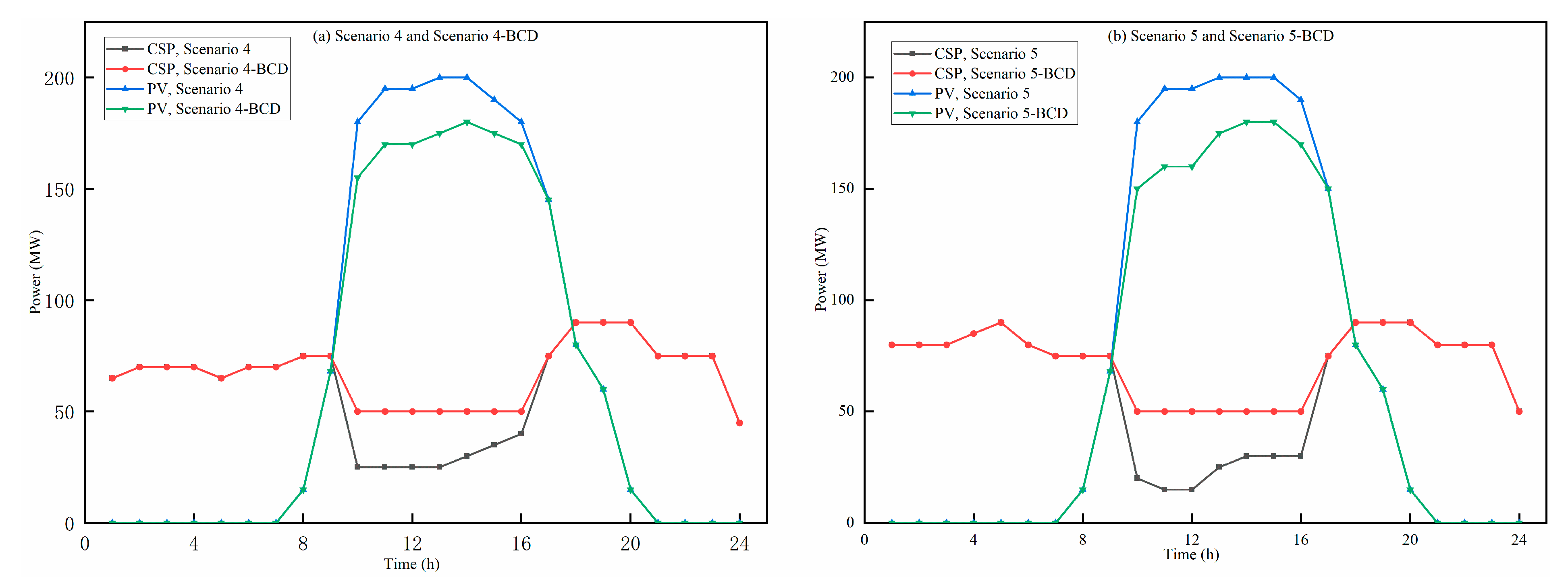
Figure 11: Dispatch comparison between original scenarios and controlled benchmark comparison dispatches during CSP deep peak regulation intervals: (a) Scenario 4 and Scenario 4-BCD; (b) Scenario 5 and Scenario 5-BCD.

The same relationship is observed in Scenario 5. In this BCD comparison, the available PV energy is 1748 MWh under both Scenario 5 and Scenario 5-BCD. Scenario 5-BCD accommodates 1563 MWh of PV generation and leaves 185 MWh of PV curtailment, whereas Scenario 5 accommodates the full 1748 MWh of available PV generation and reduces PV curtailment to zero. Therefore, relative to the controlled BCD case, CSP deep peak regulation under the complete mechanism releases 185 MWh of additional PV accommodation space and eliminates the remaining PV curtailment. This contribution is obtained under the same post-PBDR load profile and system operating conditions, so it can be attributed to the physical flexibility provided by CSP deep peak regulation rather than to a change in the load-side setting itself. The associated total PV-side CCER revenue increases by CNY 19,200, and the system operating cost decreases by CNY 282,100 relative to Scenario 5-BCD.

Comparing the two BCD analyses further shows that the PV accommodation contribution of CSP deep peak regulation increases from 145 MWh in Scenario 4 to 185 MWh in Scenario 5. This additional 40 MWh should not be interpreted as the independent PV-accommodation contribution of PBDR. Instead, it reflects the source–load coordination effect of PBDR under the dual-incentive mechanism. PBDR improves the load-side operating condition and creates a more favorable net-load profile, allowing CSP deep peak regulation to release more PV accommodation space.

Taken together, the ablation and BCD results identify three non-substitutable functions. Deep peak regulation compensation provides the direct economic signal for CSP deep peak regulation. CCER revenue sharing provides an additional carbon-value incentive linked to PV-side revenue. PBDR improves the source–load coordination condition and enhances the physical contribution of CSP deep peak regulation to PV accommodation. The complete mechanism therefore works through the coordinated interaction of load-side reshaping, CSP flexibility activation, and PV-side carbon-value allocation, rather than through any single mechanism alone.

4.4 Benchmark Comparison with Alternative Optimization and Dispatch Models

After the ablation analysis in Section 4.3, this section further compares the proposed framework with alternative uncertainty-handling methods and dispatch structures. All cases use the same modified IEEE 30-bus system, 24-h high-PV scheduling condition, PV and load forecasts, CSP–TES parameters, CCER price, network constraints, and solver settings. The proposed case corresponds to Scenario 5. The controlled benchmark settings are summarized in Table 8.

Because the model is formulated as a day-ahead scheduling problem, reserve performance is evaluated using the minimum scheduled upward reserve capacity and the number of reserve-binding periods, rather than realized reserve deployment. All models are implemented in MATLAB 2021a using YALMIP and solved by CPLEX 12.9 under the same solver tolerances.

The stochastic optimization benchmark uses 10 representative source–load scenarios with prescribed probabilities. The robust optimization benchmark adopts the same forecast-error bounds as the FCCP model but schedules against the worst-case net-load realization. The adapted literature-based multi-market benchmark adopts the CCER-sharing settlement logic of Ref. [20] while retaining the CSP–TES operating constraints used in this study. It is treated as an adapted benchmark because Ref. [20] focuses on thermal-unit deep peak regulation rather than CSP–TES operation.

4.4.1 Comparison of Uncertainty-Handling Methods

To isolate the effect of uncertainty treatment, deterministic MILP, stochastic optimization, robust optimization, and the proposed FCCP model are compared. Except for the uncertainty-handling method, the PBDR settings, CCER-sharing rules, deep peak regulation compensation, physical constraints, network constraints, and solver parameters remain unchanged.

Table 9 shows that deterministic MILP gives the lowest nominal operating cost, CNY 1.2184 million, but its minimum scheduled upward reserve capacity is only 6.8 MW. This reflects the absence of an uncertainty-aware reserve margin. Therefore, the deterministic result should be interpreted as a nominal-cost lower benchmark rather than a robust dispatch solution.

The stochastic optimization model increases the scheduled upward reserve capacity to 22.7 MW, but the operating cost rises to CNY 1.2476 million and PV curtailment reaches 9 MWh. Compared with stochastic optimization, the proposed FCCP model reduces the operating cost to CNY 1.2359 million, eliminates PV curtailment, and increases the scheduled upward reserve capacity to 28.6 MW. Its runtime is 58 s, which is slightly longer than that of the stochastic model but still acceptable for day-ahead scheduling.

Robust optimization provides the largest scheduled upward reserve capacity, 42.6 MW, but this comes with the highest operating cost, CNY 1.2926 million, higher thermal carbon emissions, and 42 MWh of PV curtailment. Compared with robust optimization, the FCCP model reduces the operating cost by CNY 56,700 and eliminates PV curtailment. These results indicate that FCCP provides a practical compromise between dispatch economy and reserve conservatism under limited-sample uncertainty.

4.4.2 Comparison of Dispatch and Settlement Structures

The second comparison evaluates the role of the proposed source–load coordination and settlement structure. The conventional single-level MILP uses the same generation and network constraints but removes the upper-level PBDR decision and fuzzy interactive coordination. The adapted literature-based multi-market benchmark adopts the CCER-sharing settlement logic from Ref. [20], while retaining the CSP–TES operating constraints used in this study. In contrast, the proposed bi-level model integrates PBDR, dynamic deep peak regulation compensation, CCER revenue sharing, PV reservation utility, and FCCP. The dispatch-performance results are summarized in Table 10, and the settlement allocation and runtime results are reported in Table 11.

Compared with the conventional single-level MILP, the proposed bi-level model reduces the system operating cost from CNY 1.2806 million to CNY 1.2359 million. PV curtailment decreases from 34 MWh to zero, thermal carbon emissions decrease by 214 tCO2, and the minimum scheduled upward reserve capacity increases from 20.1 MW to 28.6 MW.

Compared with the adapted literature-based multi-market benchmark, the proposed model further reduces the operating cost by CNY 31,500, eliminates the remaining 20 MWh of PV curtailment, reduces thermal carbon emissions by 126 tCO2, and increases the minimum scheduled upward reserve capacity from 23.5 MW to 28.6 MW. The number of reserve-binding periods also decreases from 6 to 5. These results show that the integrated source–load coordination structure improves PV accommodation, reserve adequacy, and dispatch performance.

Under the proposed model, total PV-side CCER revenue reaches CNY 181,100, compared with CNY 177,600 for the conventional single-level MILP and CNY 179,000 for the adapted benchmark. The CSP deep peak regulation compensation decreases to CNY 69,200, while the shared CCER revenue allocated to CSP increases to CNY 49,300. This indicates that the proposed mechanism does not rely only on higher ancillary-service compensation. Instead, it uses a defined share of PV-side CCER revenue as a supplementary incentive for CSP deep peak regulation.

The PV plant retains CNY 131,800 of CCER revenue under the proposed model, and the PV reservation-utility constraint remains satisfied. The runtime of the proposed model is 58 s, compared with 39 s for the conventional single-level MILP and 46 s for the adapted benchmark. The additional computation is caused by the upper-level PBDR decision and settlement coordination, but the runtime remains acceptable for day-ahead scheduling.

4.5 Convergence and Benchmark Consistency of the Solution Algorithm

To assess the convergence performance and benchmark consistency of the proposed interactive algorithm, a KKT-based relaxed benchmark is constructed for the modified IEEE 30-bus case. Because the lower-level dispatch model contains binary commitment-related variables, the KKT conditions are not used to reformulate the full MILP-based lower-level problem. Instead, the KKT-based benchmark is constructed for the continuous relaxation of the lower-level dispatch subproblem, where the binary commitment-related variables are relaxed or fixed according to the dispatch status obtained from the MILP solution. The complementary slackness conditions are linearized using the Big-M method. Therefore, this benchmark is used only as an auxiliary consistency check for the continuous dispatch subproblem, rather than as a proof of global optimality for the full bi-level MILP framework.

Fig. 12 shows the convergence process for Scenario 5. The system operating cost decreases from CNY 1.4200 million and stabilizes at approximately CNY 1.2360 million. The bi-level solution procedure meets the prescribed convergence tolerance of 10−4 after 12 iterations. This tolerance is different from the relative MIP gap used for each lower-level MILP. The final cost differs from the KKT-based relaxed benchmark by approximately 0.25%, indicating close agreement with the continuous-relaxation benchmark for this case.

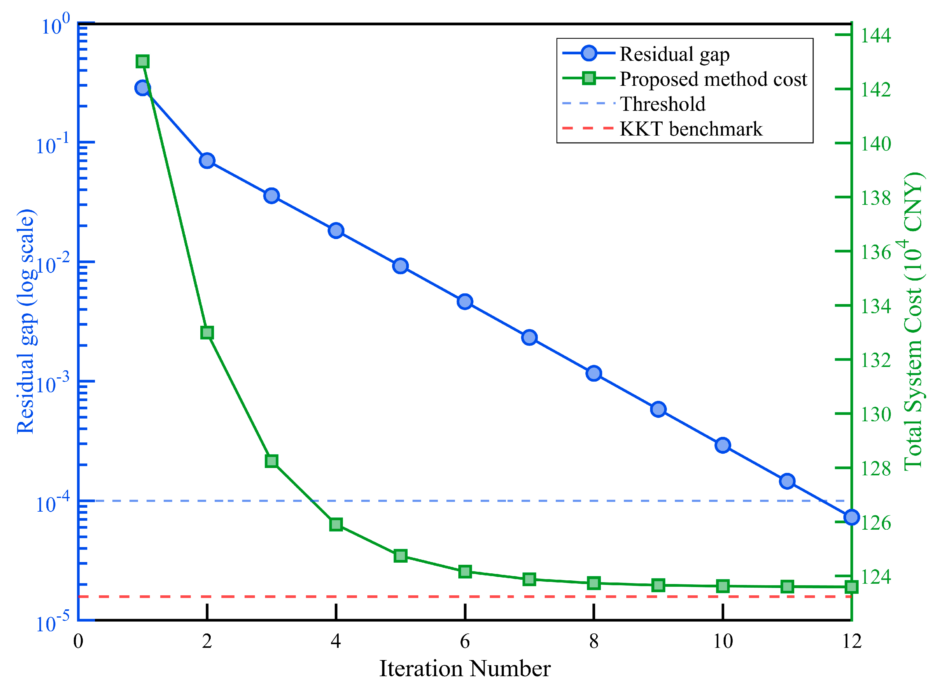
Figure 12: Convergence process of the proposed interactive algorithm and KKT-based relaxed benchmark under Scenario 5.

4.6 Sensitivity Analysis under Parameter and Price-Fluctuation Scenarios

4.6.1 Sensitivity Analysis on CCER Sharing Coefficient

Fig. 13 shows the sensitivity of system operating cost and PV net profit to the CCER sharing coefficient θ . As θ increases, a larger share of PV-side CCER revenue is allocated to the CSP plant. This strengthens the incentive for CSP deep peak regulation and reduces the system operating cost.

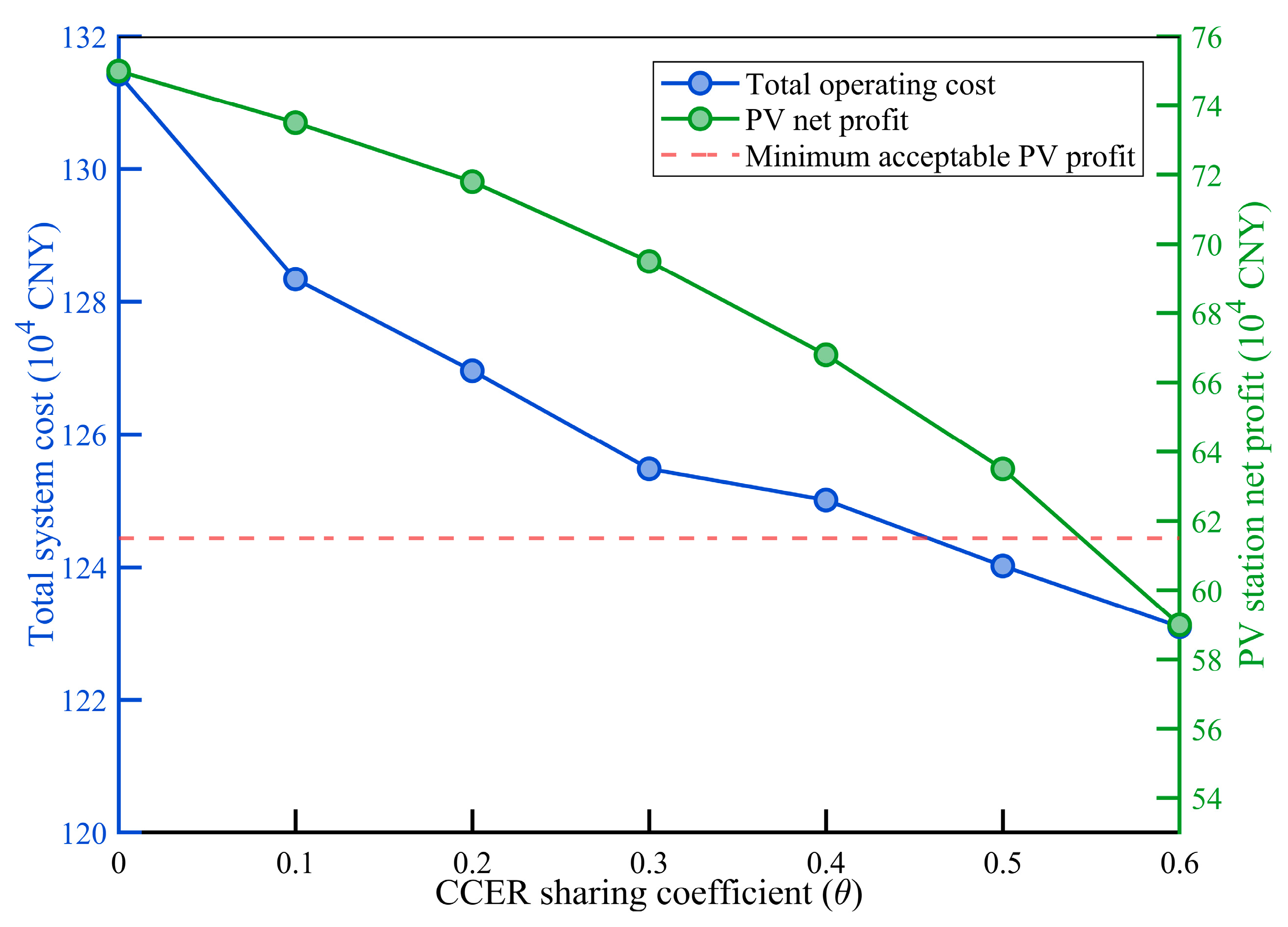
Figure 13: Sensitivity of system cost and PV net profit to the CCER sharing coefficient under Scenario 5.

However, an excessive sharing coefficient reduces the retained revenue of the PV plant and may violate its reservation-utility requirement. In the tested cases, θ = 0.5 is the largest sharing coefficient that keeps the PV net profit above the minimum acceptable level. When θ increases to 0.6, the PV net profit falls below the threshold, even though the system operating cost decreases slightly further. Therefore, θ = 0.5 is selected as the largest feasible sharing coefficient in this case.

4.6.2 Sensitivity Analysis on Thermal Storage Capacity

Fig. 14 shows the effects of TES capacity on system operating cost and total PV-side CCER revenue. When TES capacity increases from 1000 MWh to 2000 MWh, the system operating cost decreases and total PV-side CCER revenue increases. This occurs because a larger TES capacity allows the CSP plant to reduce its electrical output during high-PV periods and store more thermal energy, thereby improving PV accommodation.

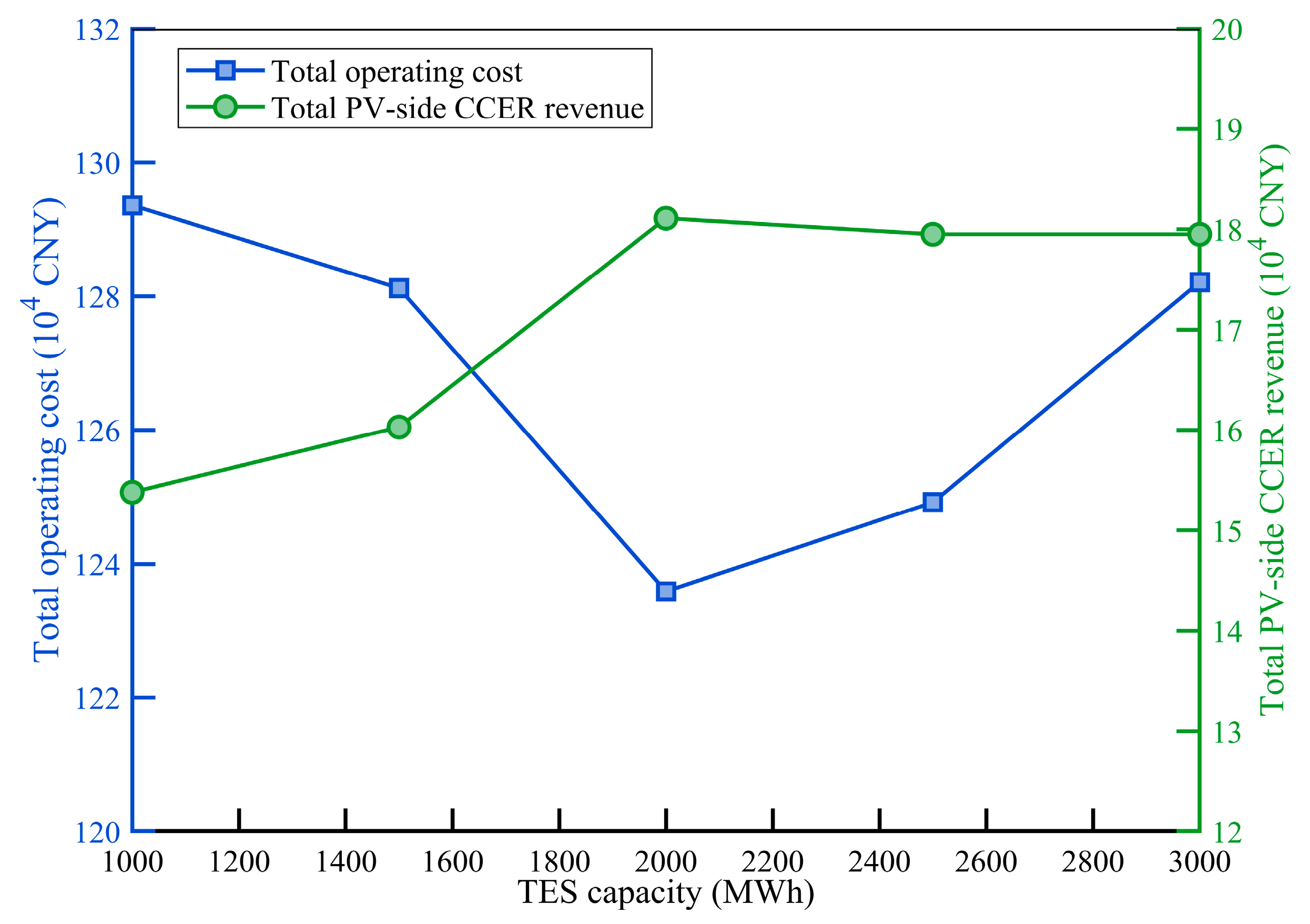
Figure 14: Sensitivity of system cost and total PV-side CCER revenue to TES capacity under Scenario 5.

When TES capacity exceeds 2000 MWh, the cost-saving effect weakens and the system operating cost begins to rise. Additional storage provides limited incremental PV accommodation, while the capital cost of TES continues to increase. Among the tested capacities, 2000 MWh gives the lowest system operating cost. Expanding beyond this level is not cost-effective under the current CSP–PV configuration and TES cost assumptions.

This result indicates that the economic value of TES capacity depends on both PV accommodation benefits and storage investment costs. If TES unit costs decline in the future, the cost-effective storage capacity may shift toward a larger value.

4.6.3 Sensitivity Analysis under Assumed CCER Price Profiles

To examine the effect of assumed CCER price levels on the revenue-sharing mechanism, a two-dimensional sensitivity analysis is conducted for the CCER sharing coefficient and the CCER price. The purpose is to identify the parameter region in which the mechanism can balance system operating-cost reduction and the economic acceptability of PV participation.

As shown in Fig. 15, the system operating cost varies with both the assumed CCER price and the sharing coefficient. Under the parameter settings used in this case, the largest feasible sharing coefficient remains θ = 0.5 across the tested CCER price range. This indicates that the selected sharing coefficient is relatively insensitive to the tested CCER price levels in the present case. However, this value should not be interpreted as a universally optimal coefficient across all market environments.

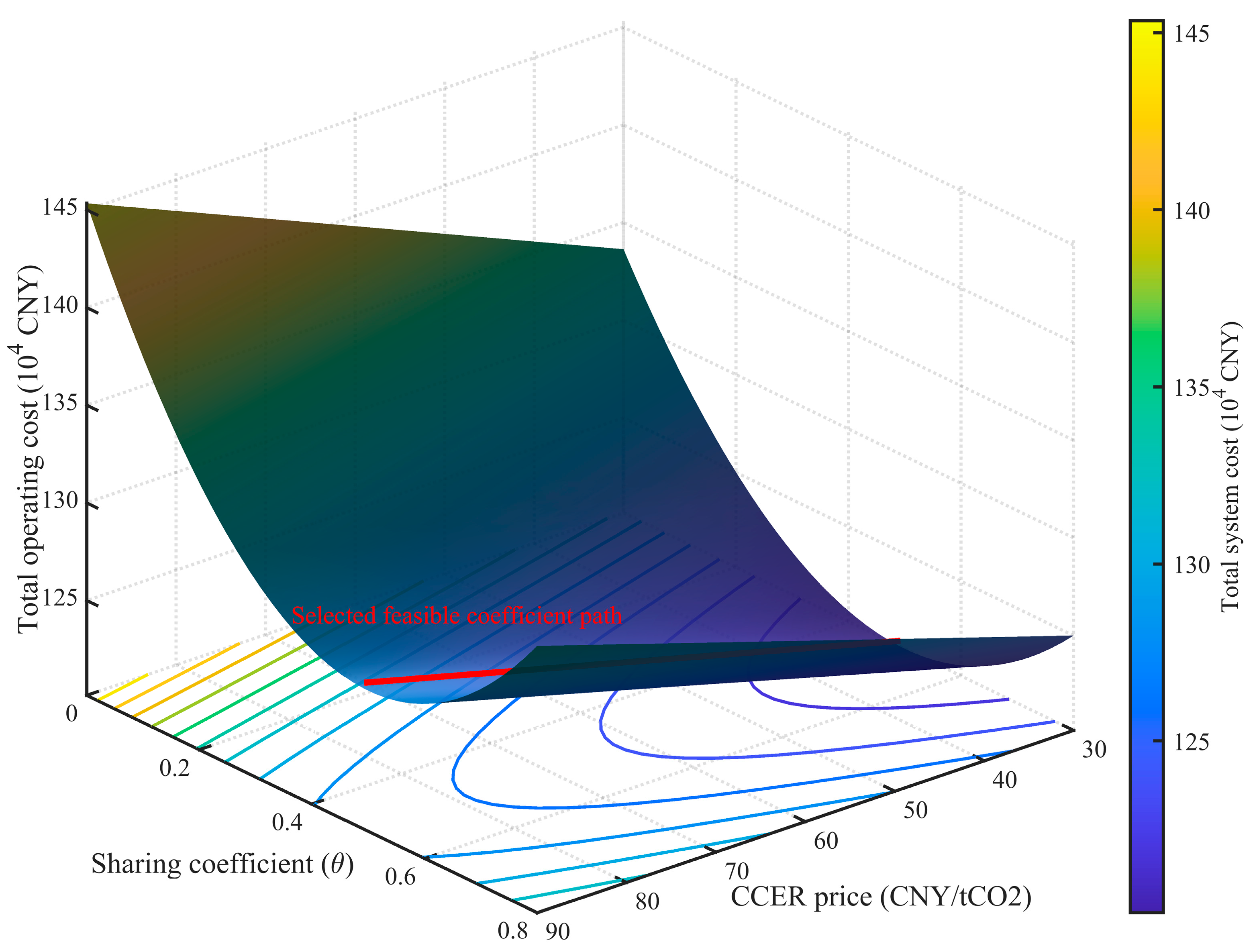
Figure 15: Joint sensitivity analysis of CCER price and sharing coefficient.

• (1)Synthetic CCER price-fluctuation scenarios and parameter settings

CCER prices may vary over time due to market and policy conditions. To examine the response of the proposed cross-market settlement mechanism to time-varying price inputs, the constant-price assumption is relaxed and three stylized CCER price scenarios are constructed. These scenarios are used as sensitivity and stress-test inputs rather than as observed CCER market-price trajectories.

Scenario A is the static-price baseline, in which the CCER price and sharing coefficient remain constant throughout the scheduling horizon.

Scenario B is a CSP-output-linked time-varying price scenario. The assumed CCER price and the allowable sharing coefficient vary over time according to the predefined CSP output profile. This scenario is used to examine the settlement response when the carbon-value incentive is temporally coupled with CSP operating conditions.

Scenario C adds random perturbations to the price profile of Scenario B. It is used as a stress-test case to examine whether the sharing mechanism remains operational under irregular assumed price fluctuations.

To formulate the dynamic sharing rule within the MILP framework, an unconstrained baseline sharing coefficient A t is first defined: At=θmin+(θmax−θmin)×pccer,t−pccer,minpccer,max−pccer,min(51) where p ccer , max and p ccer , min denote the maximum and minimum CCER prices during the forecasting period, respectively. The coefficient A t maps the price fluctuation p ccer , t into the allowable sharing range [ θ min , θ max ] .

A binary trigger variable μ t share is then introduced to link the sharing coefficient with both the carbon-price signal and the operating state of the CSP plant: 0≤θt≤M⋅μtshareθt≤At+M⋅(1−μtshare)θt≥At−M⋅(1−μtshare)(52) where μ t share indicates whether the CCER-sharing mechanism is activated. It equals 1 only when the PV plant has actual on-grid electricity and the CSP plant participates in deep peak regulation; otherwise, it equals 0. M is a sufficiently large positive constant. When μ t share = 1 , Eq. (52) enforces θ t = A t . When μ t share = 0 , the sharing coefficient is forced to zero. This formulation keeps the dynamic sharing mechanism compatible with the MILP model.

Table 12 reports the economic results under the three synthetic CCER price profiles. Compared with the static-price baseline in Scenario A, the system operating cost increases slightly from CNY 1.2359 million to CNY 1.2421 million in Scenario B and CNY 1.2489 million in Scenario C. Meanwhile, total PV-side CCER revenue increases from CNY 181,100 to CNY 183,500 and CNY 200,600, respectively.

The CSP shared CCER revenue increases from CNY 49,300 in Scenario A to CNY 51,200 in Scenario B and CNY 64,200 in Scenario C. These results indicate that the proposed sharing mechanism responds to the assumed time-varying price inputs and adjusts the settlement outcome within the specified sharing boundary.

• (2)Operational response of CSP dispatch under CSP-output-linked CCER price profiles

Fig. 16 shows the CSP dispatch profiles under the three synthetic CCER price scenarios. Because the time-varying price profiles are constructed with reference to CSP operating conditions, the figure is used to illustrate the consistency between the settlement rule and the resulting dispatch state, rather than to establish an empirical causal relationship between market prices and CSP output.

Under Scenario B, periods with higher assumed CCER prices and higher allowable sharing coefficients coincide with the predefined operating intervals in which CSP deep peak regulation is economically encouraged. When the CCER-sharing trigger is activated, the additional shared revenue helps offset the engineering-equivalent incremental cost associated with reduced heat-to-power conversion efficiency and TES thermal dissipation. Under these conditions, the CSP plant can maintain a lower electrical output or allocate more thermal energy to TES, thereby providing additional accommodation space for PV generation.

In Scenario C, random perturbations are introduced around the CSP-output-linked price profile. The dispatch results show that the CCER-sharing mechanism remains active only when the required physical and operational conditions are simultaneously satisfied, namely actual PV on-grid electricity and CSP deep peak regulation. When PV generation is unavailable, the sharing trigger is deactivated and no CCER revenue is allocated to the CSP plant.

When the assumed CCER price is lower during periods in which deep peak regulation would otherwise be encouraged, the shared revenue available to the CSP plant decreases. Consequently, the economic incentive for maintaining a deep peak regulation state becomes weaker, and the dispatch model may schedule a shallower CSP output reduction within the feasible operating range.

Overall, Fig. 16 illustrates the operational response of the proposed settlement mechanism under stylized CSP-output-linked price rules. The result should be interpreted as a sensitivity-based demonstration under assumed price inputs, not as evidence of direct price tracking in an actual CCER market.

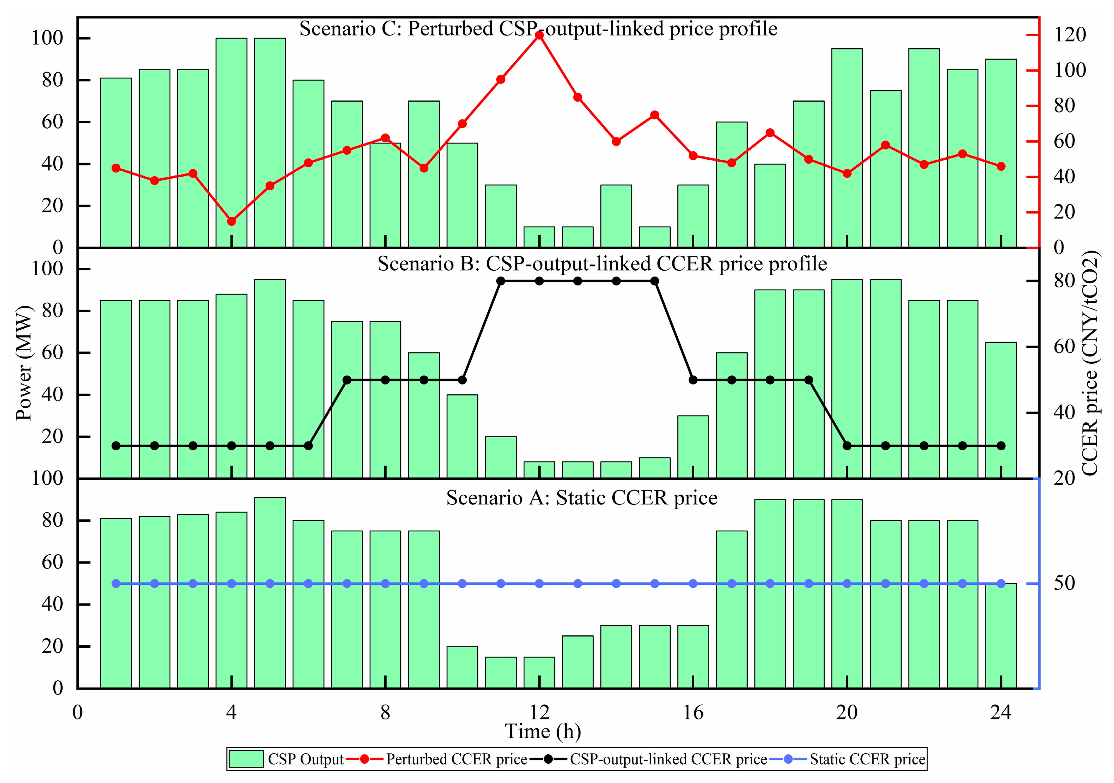
Figure 16: CSP dispatch profiles under synthetic CSP-output-linked CCER price scenarios in Scenario 5.

5 Conclusion

This paper proposes a fuzzy chance-constrained bi-level day-ahead dispatch framework for a CSP–PV system with source–load interaction, CCER-based deep peak regulation incentives, and FCCP-based uncertainty treatment. The upper level reshapes the load profile through PBDR, while the lower level coordinates thermal units, the CSP–TES system, and PV generation under network, reserve, carbon, and settlement constraints. A dual-compensation mechanism is developed by combining dynamic CSP deep peak regulation compensation with PV-side CCER revenue sharing.

The ablation results show that the three mechanisms play different roles. PBDR alone reduces the load peak-to-valley difference from 240 MW to 180 MW and the net-load peak-to-valley difference from 387.5 MW to 293.0 MW, while keeping daily electricity consumption unchanged. However, it does not independently reduce PV curtailment. This confirms that PBDR mainly smooths the load-side profile and improves the source–load coordination condition.

The controlled BCD comparisons identify the physical contribution of CSP deep peak regulation to PV accommodation. Relative to Scenario 5-BCD, CSP deep peak regulation under the complete mechanism releases 185 MWh of additional PV accommodation space and eliminates the remaining PV curtailment. The total PV-side CCER revenue increases by CNY 19,200, and the system operating cost decreases by CNY 282,100 compared with Scenario 5-BCD. These results verify that CSP deep peak regulation is the direct physical source of additional PV accommodation, while PBDR strengthens its effectiveness by creating a more favorable load-side operating condition.

The benchmark comparisons further demonstrate the value of FCCP and the complete bi-level structure. Compared with robust optimization, the FCCP model reduces operating cost by CNY 56,700 and eliminates 42 MWh of PV curtailment while maintaining 28.6 MW of upward reserve. Compared with a conventional single-level MILP model, the proposed bi-level model reduces operating cost from CNY 1.2806 million to CNY 1.2359 million, eliminates 34 MWh of PV curtailment, and reduces thermal carbon emissions by 214 tCO2.

Overall, deep peak regulation compensation, PV-side CCER revenue sharing, and PBDR are complementary rather than substitutable. The proposed framework improves PV accommodation, reserve adequacy, and settlement performance in the tested day-ahead scheduling case. Future work should validate the framework on larger systems, multiple operating days, real market-price trajectories, and post-dispatch AC power-flow checks.

References

1. Zhang Y , Zhao H , Qi Z , Li B . A two-stage low-carbon economic coordinated dispatching model for generation-load-storage resources considering flexible supply-demand balance. Appl Energy. 2024; 373: 123981. doi:10.1016/j.apenergy.2024.123981. [Google Scholar] [CrossRef]
2. Li L , Guo X , Jing R . Short-term electric load forecasting based on series decomposition and Meta-Informer algorithm. Electr Power Syst Res. 2025; 243: 111478. doi:10.1016/j.epsr.2025.111478. [Google Scholar] [CrossRef]
3. Liu G , Tomsovic K . Robust unit commitment considering uncertain demand response. Electr Power Syst Res. 2015; 119: 126– 37. doi:10.1016/j.epsr.2014.09.006. [Google Scholar] [CrossRef]
4. Štěpanec L , Koutroulis E , Aye HY , Lin OZ , Juchelkova D . How renewable energy mix shapes day-ahead price predictability: A comparative analysis of solar, wind, and biomass in Czechia. Renew Energy. 2026; 273: 126146. doi:10.1016/j.renene.2026.126146. [Google Scholar] [CrossRef]
5. Wang P , Hu B , Tai N , Zhao L , Vafai K . Peak shaving auxiliary service analysis for the photovoltaic and concentrating solar power hybrid system under the planning-dispatch optimization framework. Energy Convers Manag. 2023; 295: 117609. doi:10.1016/j.enconman.2023.117609. [Google Scholar] [CrossRef]
6. Richter P , Trimborn T , Aldenhoff L . Predictive storage strategy for optimal design of hybrid CSP-PV plants with immersion heater. Sol Energy. 2021; 218: 237– 50. doi:10.1016/j.solener.2020.11.005. [Google Scholar] [CrossRef]
7. Zhang Z , Cong W , Liu S , Li C , Qi S . Auxiliary service market model considering the participation of pumped-storage power stations in peak shaving. Front Energy Res. 2022; 10: 915125. doi:10.3389/fenrg.2022.915125. [Google Scholar] [CrossRef]
8. Wang H , Mu S , Li G , Yang Z , Yang J , Marquez FPG , et al. Modeling and operation strategy of nuclear power plant with electric heat storage in the ancillary service market. Nucl Eng Des. 2023; 415: 112686. doi:10.1016/j.nucengdes.2023.112686. [Google Scholar] [CrossRef]
9. Zhang H , Jin P , Pang W , Han P . Research on deep peaking cost allocation mechanism considering peaking demand subject and thermal power unit. Energy Rep. 2024; 12: 158– 72. doi:10.1016/j.egyr.2024.06.011. [Google Scholar] [CrossRef]
10. Cui Y , Yu SP , Zhang JT , Wang MC , Wang XB , Fu GB . Economic dispatch of high-proportion renewable energy power system considering peak-shaving compensation of concentrating solar power plant. Proc CSEE. 2023; 43( 13): 4922– 34. (In Chinese). doi:10.13334/j.0258-8013.pcsee.220054. [Google Scholar] [CrossRef]
11. Nasab MA , Alizadeh M , Nasimov R , Zand M , Nasab MA , Padmanaban S . Planning with the electricity market One day ahead for a smart home connected to the RES by the MILP method. Renew Energy Focus. 2024; 50: 100606. doi:10.1016/j.ref.2024.100606. [Google Scholar] [CrossRef]
12. Alizadeh M , Moradi Amani A , Meegahapola L , Jalili M , Hill O . Optimal traffic-informed design and operation of EV charging stations in power distribution grids. IEEE Trans Transp Electrif. 2026; 12( 3): 4375– 87. doi:10.1109/TTE.2026.3670484. [Google Scholar] [CrossRef]
13. Su X , Zhang Q , Lu Y , Hao R , Qin T , Li C , et al. Study on multi-energy scheduling strategy considering dynamic energy prices and low-carbon demand response. Renew Energy. 2025; 247: 123048. doi:10.1016/j.renene.2025.123048. [Google Scholar] [CrossRef]
14. Gao C , Lu H , Chen M , Chang X , Zheng C . A low-carbon optimization of integrated energy system dispatch under multi-system coupling of electricity-heat-gas-hydrogen based on stepwise carbon trading. Int J Hydrogen Energy. 2025; 97: 362– 76. doi:10.1016/j.ijhydene.2024.11.055. [Google Scholar] [CrossRef]
15. Yang S , Mi F . Renewable portfolio standards, carbon emissions trading and China certified emission reduction: The role of market mechanisms in optimizing China’s power generation structure. Energies. 2025; 18( 4): 894. doi:10.3390/en18040894. [Google Scholar] [CrossRef]
16. Zhang X , Guo X , Zhang X . Mutual conversion mechanisms for environmental interest products to jointly enhance synergistic effect between power, CET and TGC markets in China. Energy Econ. 2024; 131: 107311. doi:10.1016/j.eneco.2024.107311. [Google Scholar] [CrossRef]
17. Zhang C , Lin B . Impact of introducing Chinese certified emission reduction scheme to the carbon market: Promoting renewable energy. Renew Energy. 2024; 222: 119887. doi:10.1016/j.renene.2023.119887. [Google Scholar] [CrossRef]
18. Yang J , Lei L , Liu D , Luo W . A distributed dispatch approach for district-level electric-heat-gas integrated energy systems considering carbon emission and green certificate trading. Electr Power Syst Res. 2025; 244: 111541. doi:10.1016/j.epsr.2025.111541. [Google Scholar] [CrossRef]
19. Mathuria P , Bhakar R , Li F . GenCo’s optimal power portfolio selection under emission price risk. Electr Power Syst Res. 2015; 121: 279– 86. doi:10.1016/j.epsr.2014.11.006. [Google Scholar] [CrossRef]
20. Yang YD , Gao HJ , Liu TJ , Guo MH , He W . Low carbon dispatch of power system considering CCER revenue sharing incentive for deep peak-shaving of thermal power units. Electr Power Autom Equip. 2024; 44( 9): 121– 8. (In Chinese). doi:10.16081/j.epae.202403026. [Google Scholar] [CrossRef]
21. Xiong H , Xiang TY , Chen HK , Lin F , Su JH . Research of fuzzy chance constrained unit commitment containing large-scale intermittent power. Proc CSEE. 2013; 33( 13): 36– 44. (In Chinese). doi:10.13334/j.0258-8013.pcsee.2013.13.003. [Google Scholar] [CrossRef]
22. Liu B , Zhao R , Wang G . Uncertain programming and its applications. Beijing, China: Tsinghua University Press; 2003. (In Chinese). [Google Scholar]
23. Wood AJ , Wollenberg BF , Sheblé GB . Power generation, operation, and control. 3rd ed. Hoboken, NJ, USA: John Wiley & Sons, Inc.; 2013. 656 p. [Google Scholar]
24. Albadi MH , El-Saadany EF . A summary of demand response in electricity markets. Electr Power Syst Res. 2008; 78( 11): 1989– 96. doi:10.1016/j.epsr.2008.04.002. [Google Scholar] [CrossRef]
25. Villacrés R , Carrión D . Optimizing real and reactive power dispatch using a multi-objective approach combining the ϵ-constraint method and fuzzy satisfaction. Energies. 2023; 16( 24): 8034. doi:10.3390/en16248034. [Google Scholar] [CrossRef]
26. Zimmerman RD , Murillo-Sánchez CE , Thomas RJ . MATPOWER: Steady-state operations, planning, and analysis tools for power systems research and education. IEEE Trans Power Syst. 2011; 26( 1): 12– 9. doi:10.1109/TPWRS.2010.2051168. [Google Scholar] [CrossRef]
27. Anderson KS , Hansen CW , Holmgren WF , Jensen AR , Mikofski MA , Driesse A . Pvlib Python: 2023 project update. J Open Source Softw. 2023; 8( 92): 5994. doi:10.21105/joss.05994. [Google Scholar] [CrossRef]
Cite This Article
Copyright © 2026 The Author(s). Published by Tech Science Press.
This work is licensed under a Creative Commons Attribution 4.0 International License , which permits unrestricted use, distribution, and reproduction in any medium, provided the original work is properly cited.
Downloads
Citation Tools