
 Login
Login Register
 Submit a Paper
 Propose a Special lssue
 Open Access
ARTICLE
Data-Driven Differential Energy Forecasting for Controlled Environmental Chambers
1 College of Urban Rail Transit and Logistics, Beijing Union University, Beijing, China
2 School of Airport Economy and Management, Beijing Institute of Economics and Management, Beijing, China
* Corresponding Author: Jingyun Liu. Email:
Energy Engineering 2026, 123(11), 24 https://doi.org/10.32604/ee.2026.088401
Received 02 July 2026; Accepted 07 September 2026; Issue published 24 September 2026
 View Full Text
 Download PDF
Abstract
Controlled environmental chambers require continuous cooling, heating, humidification, ventilation and lighting to maintain stable indoor conditions, resulting in intensive and fluctuating energy demand. This study proposes a data-driven workflow for short-term differential energy consumption prediction in a BAE20-series controlled environmental chamber manufactured by Beijing Chuangyi Xintong Technology Co., Ltd. (Beijing, China) to support low-carbon operation and operational diagnostics. Chamber monitoring data were preprocessed to construct differential energy consumption, with negative differences set to zero and 99.5th-percentile (P99.5) truncation applied to reduce extreme spike effects. The resulting target series showed high sparsity, local spikes, short-term inertia and periodicity. Ridge regression, Random Forest, baseline Extreme Gradient Boosting (XGBoost), an improved XGBoost workflow, recurrent neural network baselines, autoregressive integrated moving average (ARIMA) and simple statistical baselines were evaluated using five-fold time-series validation and unified metrics. The improved XGBoost workflow achieved the lowest errors in the principal model comparison, with mean absolute error (MAE), root mean square error (RMSE), and coefficient of determination (R2) values of 0.0001 ± 0.0001, 0.0008 ± 0.0005 and 0.9981 ± 0.0025, respectively. Under a separate expanding-window ablation with chronological data partitioning, eleven sensor-derived physical features reduced mean MAE by 17.00% and RMSE by 8.82% across all five folds. Unified-feature and ablation experiments indicate that the improvement mainly arises from robust target processing, rolling statistical features, time-series feature representation and regularized training, rather than model type alone. These findings suggest that energy prediction for controlled laboratory environments should align target construction and feature representation with sparse differential energy dynamics, offering a practical basis for low-carbon operation, anomaly detection and future control-oriented energy management.Keywords
Supplementary Material
Supplementary Material FileEnergy management in buildings and controlled facilities is increasingly moving from retrospective statistics toward prediction, diagnosis, and operational optimization based on monitoring data [1]. Controlled environmental chambers must maintain stable temperature, humidity, carbon dioxide (CO2) concentration, and illuminance over long periods, while their energy consumption is affected by outdoor conditions, equipment start-stop behavior, control strategies, and experimental operating states. Related heating, ventilation and air conditioning (HVAC) and controlled-environment studies show that temperature, humidity, ventilation, and control strategies are closely associated with energy performance under regulated indoor conditions [2,3,4]. Model-predictive and greenhouse-control studies further emphasize temperature-humidity modeling in regulated environments [5,6]. Previous building and HVAC studies have also shown that monitoring, prediction, and control-oriented analysis can support energy-saving operation, anomaly diagnosis, and energy management [7,8]. Compared with whole-building datasets, the chamber records examined here have high sampling frequency, clear control boundaries, and concentrated environmental variables, making them suitable for analyzing the relationship between environmental conditions and energy-consumption changes under controlled operation.
Existing energy prediction studies mainly rely on physics-based or data-driven models. Physics-based models provide stronger physical interpretability, but they often require parameter assumptions and calibration steps when operating states change frequently or multiple variables are coupled [9,10]. Data-driven methods can learn mappings between environmental variables and energy consumption from monitoring data and have been widely used in hourly building energy prediction and feature-based load analysis [7,11]. Broader model-applicability and residential prediction studies have also compared multiple machine-learning paradigms for building energy consumption prediction [12]. However, most available studies focus on whole-building loads or cumulative energy consumption. Research on small-scale, high-frequency, controlled-environment operational data remains limited, especially for short-period differential energy consumption, where sparsity, local spikes, and time dependence strongly affect prediction performance.
This study uses operational monitoring data from a BAE-series controlled environmental chamber. The records were exported from sensors, electricity meters, and programmable logic controller-human-machine interface (PLC-HMI) historical logs, including indoor temperature, humidity, dew-point temperature, CO2 concentration, illuminance, outdoor temperature, and cumulative electricity meter readings. To address missing values, abnormal codes, communication errors, and local spikes, the workflow standardizes time fields, imputes missing values, detects anomalies, normalizes numerical variables, and constructs differential energy consumption from cumulative electricity readings to represent load changes between successive cleaned records. This data-quality treatment is consistent with the need for anomaly detection, repair, and preprocessing in monitored building-energy datasets [8,13,14].
To evaluate data quality and modeling applicability, this study further analyzes sparsity characteristics, stationarity, autocorrelation, time-aggregation patterns, and baseline prediction performance. The dataset and processing workflow support short-period energy prediction, abnormal fluctuation detection, time-series feature analysis, and model adaptability evaluation for controlled environmental chambers. The main contribution of this study is to provide a reproducible differential energy consumption prediction workflow for controlled environmental chambers, linking operational data processing, target construction, feature representation, and model validation for low-carbon operation and future control-oriented energy management.
Recent studies provide three useful comparison lines. Building-load forecasting reviews emphasize preprocessing, feature selection, and historical-load representation [15]. HVAC-specific evidence further shows that data preprocessing and input selection materially affect predictive performance [14]. Intermittent-series studies separately address sparse event occurrence and magnitude [16] and robust recurrent forecasting [17]. Cold-storage forecasting integrates environmental and temporal variables into machine-learning pipelines [18], whereas controlled-environment optimization couples temperature, humidity, CO2, lighting, and control states [19]. Their objectives and data structures, however, differ from successive-record differential meter readings with many zeros and occasional spikes. A structured comparison of representative studies is provided in Table 1.
Table 1: Structured comparison of representative Energy-Forecasting studies.
| Study | Temporal Resolution | Target Variable | Input Features | Sparsity Handling | Main Method | Application and Limitation |
|---|---|---|---|---|---|---|
| Zhang et al. [15] | Multiple (review) | Building load | Weather, schedules and historical load | Reviewed indirectly | machine-learning review | Broad building scale; no chamber-scale differential target |
| Xiao et al. [14] | Study-specific HVAC records | HVAC energy | Operational and environmental variables | Preprocessing and feature selection; no event model | Deep learning | Comparatively continuous HVAC consumption |
| Türkmen et al. [16] | Series-dependent event intervals | Event occurrence and magnitude | Event history and elapsed time | Explicit intermittent-event formulation | Deep renewal process | General intermittent series; no chamber sensor coupling |
| Jeon and Seong [17] | Benchmark-dependent | Intermittent observations | Historical series | Robust recurrent formulation | Recurrent network | No environmental-variable coupling |
| Alkhulaifi et al. [18] | Hourly operational records | Energy, temperature and humidity | Environment, weather and temporal features | Feature engineering; no zero-inflated objective | Extreme Gradient Boosting regression/Random Forest regression pipeline | Cold-storage facility rather than successive-record chamber increments |
| Chen et al. [19] | Dynamic control simulation | Climate and energy-control objectives | Temperature, humidity, CO2, lighting and control states | Not applicable to a sparse meter target | nonlinear model predictive control | Control-oriented simulation rather than meter forecasting |
| Bahramnia et al. [5] | Study-specific HVAC series | Temperature-humidity control | Indoor and outdoor environmental states | Not explicitly addressed | Model predictive control | Building HVAC control context |
| Wang et al. [11] | Short-term monitoring interval | Building energy | Historical and operational features | Not explicitly addressed | Gradient-boosted regression trees | Building-level rather than chamber-level prediction |
| Wang et al. [20] | Operational cold-storage records | Cold-storage energy | Operating and environmental variables | Not explicitly addressed | Optimized LSTM | Facility energy target; no successive-record sparse increments |
| Present study | High-frequency records with repeated timestamp labels | Differential energy increment | Six sensors, historical, calendar and physical-proxy features | Fold-specific cap and historical non-zero counts | Linear, tree, recurrent and statistical comparisons | Single chamber; successive-record target with chronological and multi-step validation |
As summarized in Table 1, prior work seldom combines a high-frequency, successive-record, highly sparse energy-increment target with chamber environmental states, strictly historical feature construction and direct comparison across linear, tree, recurrent and statistical baselines. The present study addresses this narrower gap through fold-specific target processing, chronological validation and physically informed sensor features. The forecasts are intended for short-horizon monitoring, anomaly screening, maintenance scheduling, and load management within the defined chamber application scope. At the policy level, facility-scale efficiency measures can complement broader instruments that encourage technological innovation and sustainable-energy transitions [21].
The dataset was collected from a BAE-series controlled environmental chamber. The original records were acquired by sensors, electricity meters, and the PLC-HMI system, and were exported as comma-separated values (CSV) files from the historical records of the touch-screen interface. The data mainly include chamber environmental variables, outdoor temperature, and cumulative electricity meter readings, where the cumulative electricity readings are used to construct the differential energy consumption variable. The collected variables and their descriptions are summarized in Table 2. Because the original records contain missing values, abnormal codes, and communication errors, with some abnormal values represented by extreme numbers such as −30,000, unified cleaning and variable standardization are required in subsequent processing.
Unless otherwise specified, all figures and tables presenting experimental data, statistical analyses, model outputs, and derived results were generated by the authors based on the chamber monitoring records and the analyses conducted in this study.
Table 2: Description of collected data.
| Parameters | Description |
|---|---|
| Time, s | Timestamp of data acquisition |
| Indoor temperature, °C | Internal air temperature of the controlled environmental chamber |
| Indoor relative humidity, % | Internal air humidity of the controlled environmental chamber |
| Indoor CO2 concentration, ppm | Gas concentration level |
| Indoor illuminance, lx | Indoor light intensity |
| Indoor dew point, °C | Dew-point temperature of chamber air |
| Outdoor temperature, °C | External ambient temperature |
| Cumulative electricity meter reading, kWh | Total meter reading |
2.2 Data Preprocessing and Data Partitioning
To improve data consistency and reusability, this study applied a unified preprocessing procedure to the original CSV records. First, the time field was formatted, and time-derived variables including year, month, day, hour, minute, weekday, and weekend indicator were extracted. Numerical fields were then standardized using Z-score normalization to reduce the influence of different units and scales on subsequent analysis and modeling.
For missing values and anomalies in the original records, k-nearest neighbors (KNN) was used for missing-value imputation, and K-means clustering combined with a distance threshold was used to identify outlying samples. If the distance from a sample to its assigned cluster center exceeded the predefined threshold, the sample was identified as an anomaly and removed.
For energy variables, the cumulative electricity meter readings were chronologically ordered and transformed into successive-record differential energy consumption. Each valid target value is the non-negative difference between two consecutive cleaned records and is expressed in kWh per record transition; repeated timestamp labels are retained as separate observations because no minute-level aggregation is applied. Negative differences were set to zero, and P99.5 truncation was applied to reduce the influence of extreme spikes. The basic structure of the preprocessed dataset is summarized in Table 3. The descriptive statistics of the main environmental and energy variables are presented in Table 4, while the sparsity and truncation characteristics of differential energy consumption are summarized in Table 5.
Table 3: Overview of the preprocessed data.
| Item | Value |
|---|---|
| Time range (after preprocessing) | 11 March 2025 12:45 to 17 July 2025 18:14 |
| Total cleaned record rows | 212,102 |
| Unique timestamp labels in the Time field | 105,830 |
| Mean record rows per unique timestamp label | 2.004 (=212,102/105,830) |
| Candidate successive-record transitions | 212,101 (the first record has no predecessor) |
| Differential-energy target | Non-negative difference between successive cleaned cumulative-meter records |
| Median interval between successive unique timestamp labels | 1 min |
| Target and pointwise-error unit | kWh per valid record transition |
| Number of fields (columns) | 17 |
| Number of numerical fields (columns) | 16 |
Table 4: Descriptive statistics of main variables.
| Variable | Mean | Standard Deviation | Minimum | Median | Maximum |
|---|---|---|---|---|---|
| Indoor temperature, °C | 15.47 | 8.49 | −0.03 | 15.25 | 30.57 |
| Indoor humidity, %RH | 71.96 | 9.09 | 31.94 | 75.63 | 95.27 |
| Indoor dew point, °C | 10.27 | 7.75 | −8.65 | 11.57 | 25.28 |
| Indoor CO2 concentration, ppm | 501.56 | 77.08 | 324 | 490 | 890 |
| Indoor illuminance, Lux | 195.86 | 28.6 | 142 | 196 | 308 |
| Outdoor temperature, °C | 25.63 | 5.74 | 1.93 | 26 | 48.31 |
| Cumulative electricity meter reading, kWh | 1197.66 | 271.35 | 617.7 | 1215.1 | 1661.8 |
Table 5: Sparsity and truncation statistics of differential energy consumption.
| Statistic | Value |
|---|---|
| Mean successive-record differential energy, kWh per record transition | 0.0055 |
| Standard deviation of successive-record differential energy, kWh per record transition | 0.0881 |
| Maximum successive-record differential energy, kWh per record transition | 25.1 |
| Proportion of zero successive-record differences | 95.05% |
| Number of negative successive-record meter differences | 1313 |
| P99.5 truncation threshold, kWh per record transition | 0.1 |
| Number of transitions above P99.5 | 41 (0.019%) |
2.3 Data Visualization Analysis
To present the basic structure of the dataset, this study plotted the energy consumption series and the distributions of the main environmental variables, as shown in Fig. 1 and Fig. 2. Cumulative Electricity Meter Reading generally increased over time, while differential energy consumption exhibited a structure with many zero values and a small number of spikes. Indoor temperature, humidity, and dew point were relatively concentrated, whereas CO2 concentration, illuminance, and outdoor temperature showed higher dispersion. These results indicate that the dataset contains both stable environmental control processes and local energy-consumption fluctuations, supporting subsequent data quality validation and reuse analysis.
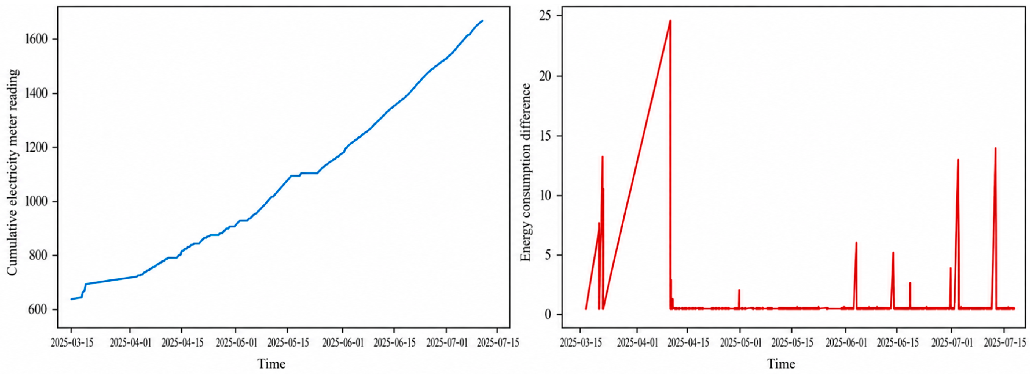
Figure 1: Comparison of cumulative electricity meter reading and differential energy consumption time series.
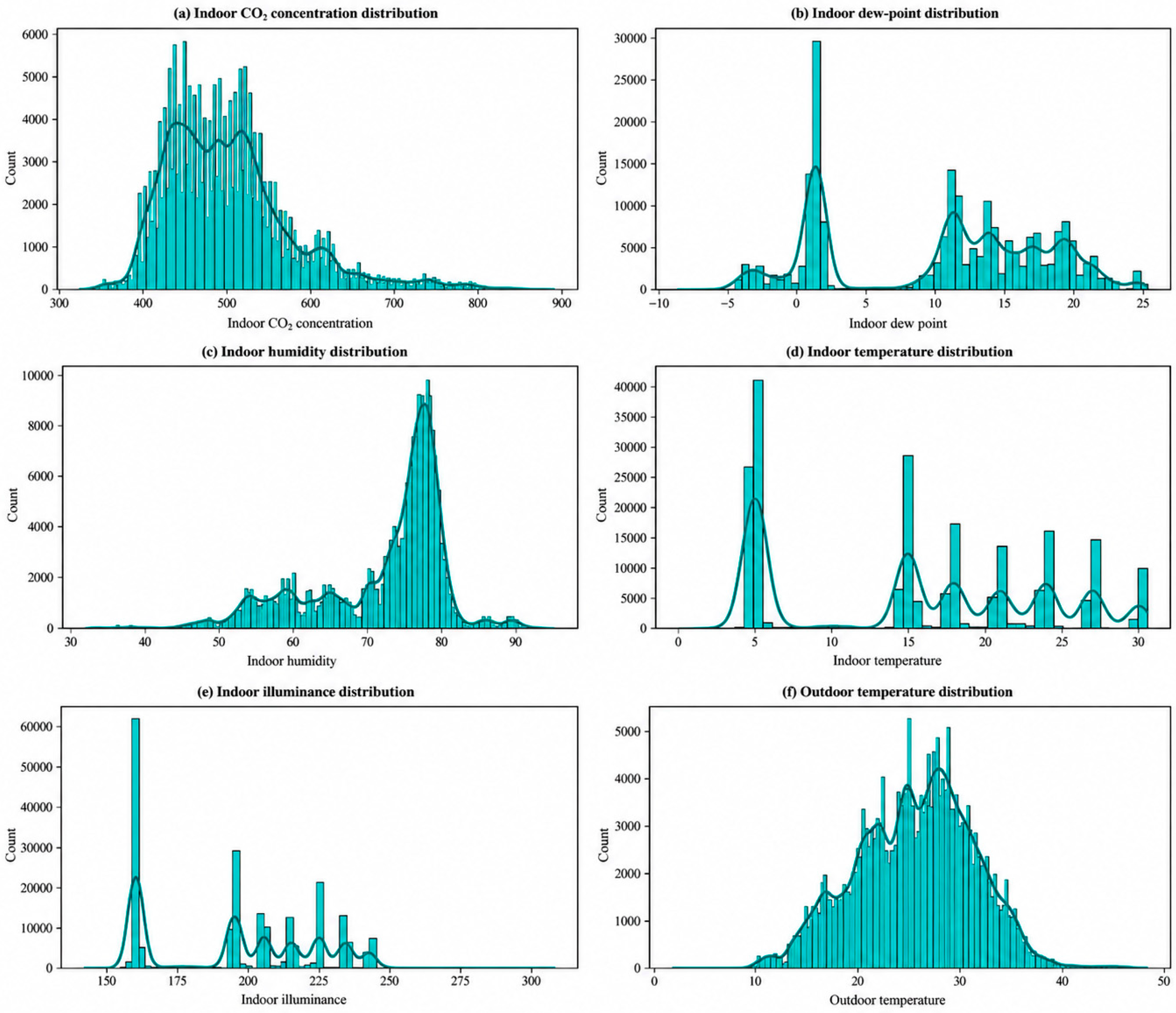
Figure 2: Distribution characteristics of main environmental variables.
2.4 Time-Series Quality Validation
To validate the time-series characteristics of the differential energy consumption variable, this study conducted Augmented Dickey–Fuller (ADF) and Kwiatkowski–Phillips–Schmidt–Shin (KPSS) stationarity tests, autocorrelation analysis, and time-aggregation analysis for Cumulative Electricity Meter Reading and differential energy consumption. The results show that Cumulative Electricity Meter Reading has an obvious trend component. After differencing, the unit-root characteristics are substantially weakened, but the series is still affected by many zero values, local spikes, and operating-state transitions, and therefore remains not fully stationary. The mean differential energy consumption is 0.0055 kWh per record transition, the zero-value ratio is 95.05%, the maximum value is 25.1 kWh per record transition, and the P99.5 truncation threshold is 0.1 kWh per record transition, indicating that this variable has high sparsity and long-tailed spike characteristics.
The autocorrelation function (ACF) and partial autocorrelation function (PACF) results show that differential energy consumption has the strongest correlation at the one-record lag, maintains a relatively high correlation at the 24-record lag, and exhibits a clear decline after the 48-record lag. The time-aggregation results further indicate that energy consumption changes are related to operating rhythms, lighting adjustment, and outdoor environmental variation. These results show that the dataset contains short-term inertia, periodicity, and local abrupt changes, and can support short-period energy prediction, abnormal fluctuation detection, and time-series feature analysis. The stationarity test results are reported in Table 6, and the corresponding time-series validation results are shown in Fig. 3.
Table 6: Stationarity test results for raw cumulative electricity meter reading and differential energy consumption.
| Series | ADF Statistic | ADF p-Value | KPSS Statistic | KPSS p-Value |
|---|---|---|---|---|
| Raw cumulative electricity meter reading | −2.073 | 0.256 | 78.624 | 0.01 |
| Differential energy consumption | −36.256 | 0 | 10.399 | 0.01 |
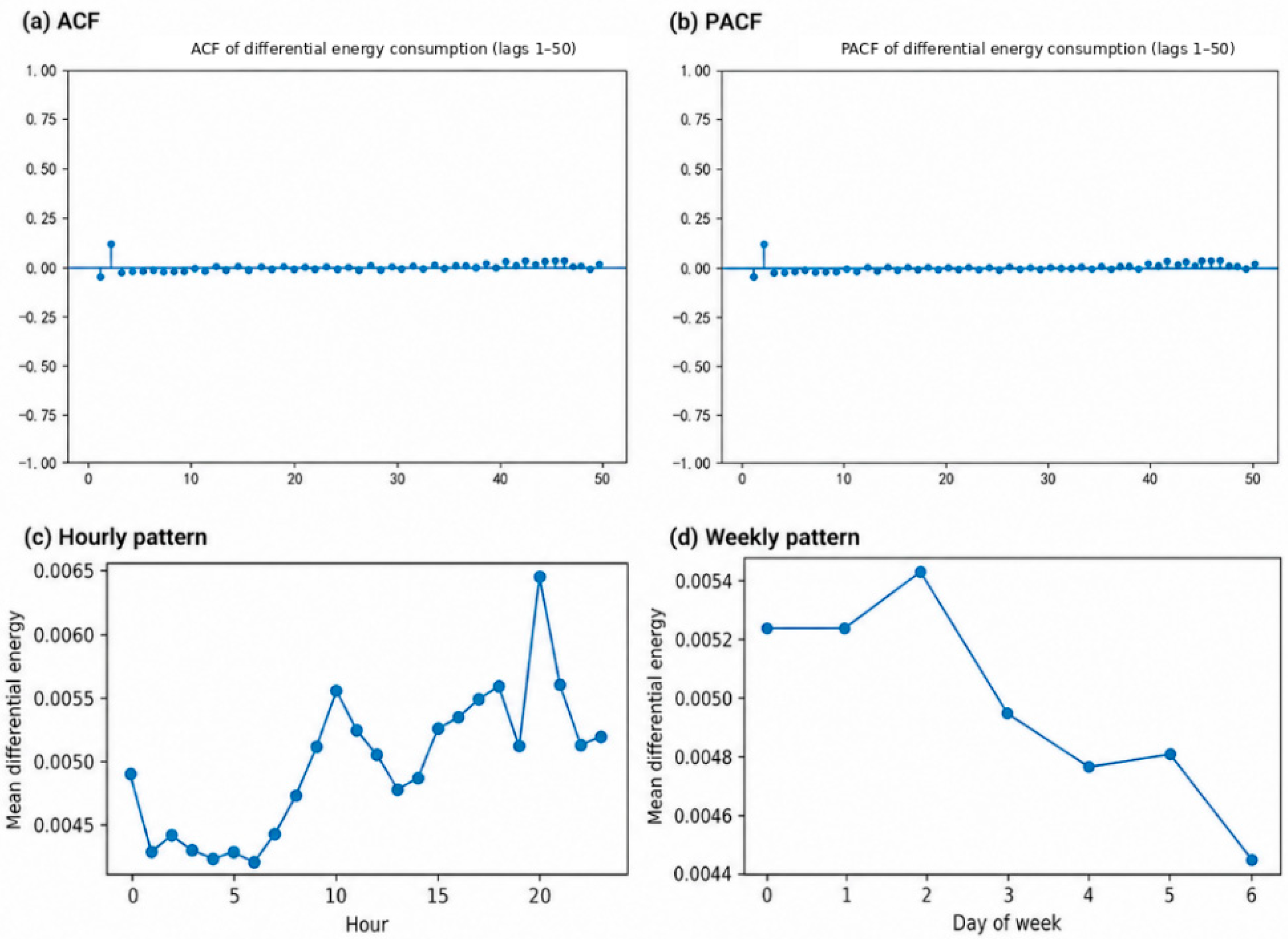
Figure 3: Validation of Time-Series characteristics of differential energy consumption.
3 Prediction Models and Evaluation Methods
3.1 Theoretical Background and Modeling Rationale
The short-period energy response of a controlled environmental chamber can be interpreted through a coupled load-control chain. Indoor-outdoor temperature differences represent sensible thermal demand; relative humidity, dew-point depression, vapor-pressure deficit and absolute humidity describe moisture-related demand; and CO2 concentration and illuminance reflect air-quality and lighting-related operating conditions. HVAC and controlled-environment studies support the dependence of equipment energy use on thermal, moisture and control conditions [2,3,4,5,6,19].
The present study characterizes chamber energy behavior through monitored environmental states, cumulative meter readings, and sensor-derived physical quantities. These variables describe thermal, moisture, air-quality, lighting, and operating-condition changes that are directly relevant to chamber conditioning demand. Accordingly, they are used as physically interpretable descriptors in the forecasting framework to link environmental dynamics with short-period differential energy consumption.
Differential energy consumption represents the non-negative increment between successive cleaned cumulative-meter records. Lagged values describe short-term persistence, rolling statistics describe local intensity and volatility, and historical non-zero counts describe recent event frequency in the sparse target. XGBoost is used to learn nonlinear interactions among these environmental, temporal and historical descriptors, while regularization and chronological validation constrain model complexity and evaluation bias.
To validate the usability of the dataset for short-period differential energy consumption prediction, this study selected Ridge regression, Random Forest, XGBoost, a recurrent neural network (RNN), and ARIMA as reuse examples, and supplemented them with two simple baselines: Naive last and Historical mean. These models represent linear mapping, static nonlinear modeling, gradient-boosted trees, sequence neural networks, traditional univariate time-series modeling, and simple statistical prediction, respectively. Previous building-energy studies have used regression, tree-based, and gradient-boosting methods for model applicability analysis and short-term prediction [7,11,12]. Related residential, cold-storage, and refrigerated-system studies further provide references for machine-learning and neural-network-based energy or load prediction [12,18,21]. These models are used here to examine the support provided by the dataset for different prediction methods.
Ridge regression is used as a linear reference model and constrains model complexity through L2 regularization. Its objective function can be expressed as:
Random Forest characterizes the nonlinear relationship between environmental variables and differential energy consumption through the ensemble averaging of multiple regression trees. Its prediction form can be expressed as:
XGBoost introduces a gradient-boosting mechanism on the basis of tree models and improves the model representation of complex nonlinear relationships by iteratively fitting residuals. Its objective function can be expressed as:
The recurrent neural network baseline uses historical sequences as sliding-window inputs to examine the applicability of explicit sequence modeling to this dataset. Its state-update process can be summarized as:
In addition, ARIMA is introduced as a traditional univariate time-series baseline. This model uses only the historical information of the differential energy consumption series for prediction and does not include indoor or outdoor environmental variables. It is used to examine the autoregressive predictability of the target series itself. Based on the stationarity test results in Section 2.4, this study uses differential energy consumption as the modeling target, sets d = 0, and selects the model order within a low-order candidate range using the Akaike information criterion (AIC) and Bayesian information criterion (BIC).
The above models are mainly used as technical validation and reuse examples for the dataset, with the aim of evaluating the predictability and adaptability differences of differential energy consumption data under different modeling paradigms.
To validate the usability of the dataset for differential energy consumption prediction, this study compares linear models, tree models, boosted tree models, recurrent neural networks, and simple baselines. All models use differential energy consumption as the prediction target and are evaluated with unified metrics for prediction error and goodness of fit. The main model settings are shown in Table 7.
Table 7: Main training settings of the models.
| Model | Inputs and Features | Training Settings |
|---|---|---|
| Ridge regression | Environmental variables, lagged differential energy consumption, and rolling statistical features | StandardScaler; α = 1.0; five-fold time-series validation |
| Random forest | Main environmental variables and differential energy consumption | n_estimators = 200; random_state = 42; five-fold time-series validation |
| XGBoost (baseline) | Environmental variables, simple lag terms, and moving average | n_estimators = 500; learning_rate = 0.05; max_depth = 6; KFold, shuffle = False |
| XGBoost (improved) | Environmental variables, multi-order lags, rolling statistics, non-zero windows, and time-derived variables | eta = 0.04; max_depth = 5; min_child_weight = 12; L2 regularization; early stopping; TimeSeriesSplit |
| Recurrent neural network baseline | Environmental-variable sequence input, sequence length = 24 | gated recurrent unit/long short-term memory (GRU/LSTM); units = 64/32; Dropout = 0.2; Adam; early stopping and learning-rate decay |
| ARIMA | Univariate differential energy consumption series | Parameter range set based on ADF and ACF/PACF results; order selection by AIC/BIC; five-fold time-series validation |
| Simple baselines | Historical differential energy consumption | Naive last; Historical mean; same evaluation metrics as the main models |
This study positions the XGBoost application optimization scheme as a modeling-workflow optimization tailored to the characteristics of controlled environmental chamber differential energy consumption. It mainly focuses on robust target processing, time-series feature construction, and training stability control. The emphasis on feature construction and controlled-environment energy modeling is consistent with previous studies on building-load prediction, HVAC preprocessing, cold-storage forecasting, and controlled-environment optimization [14,15,18,19,21]. ARIMA uses only the historical differential energy consumption series and serves as a traditional univariate time-series baseline, providing a contrast to supervised learning models that incorporate environmental variables and time-series feature engineering. The main training settings of the recurrent neural network baseline are summarized in Table 7, and the complete hyperparameter and training-control configuration is provided in Supplementary Table S1. The detailed feature construction and workflow design of the improved XGBoost model are summarized in Table 8.
Table 8: Feature construction for the improved XGBoost model.
| Design Component | Construction Method | Corresponding Data Characteristic | Function |
|---|---|---|---|
| robust target processing | Cumulative-electricity differencing, negative values set to zero, and P99.5 percentile truncation | Cumulative electricity has a clear trend; differential energy contains negative values and a small number of spikes | Represents short-period load changes and reduces the disturbance of abnormal peaks |
| Time-series features | Multi-order lag terms, rolling mean, and rolling standard deviation | ACF/PACF show short-term correlation and local fluctuations in the series | Captures short-term inertia and local operating-state changes |
| Sparsity features | Nonzero-window statistics | Differential energy has a high zero-value ratio and sparse nonzero points | Indicates whether recent periods are in an active energy-change stage |
| Periodic features | Hour, weekday, and weekend indicator | Time-aggregation results show intra-day and weekly differences | Represents operating rhythms and periodic disturbances |
| Training control | Smaller learning rate, L2 regularization, and early stopping | The differential target is noisy and sensitive to spikes | Controls model complexity and improves cross-fold stability |
Physical-Feature, Mathematical-Variable and Model-Input Mapping
For the temporal robustness, sensitivity, feature-importance and physical-feature analyses, each training window preceded its test window. The P99.5 cap was estimated from the corresponding training portion only, and all lagged, rolling and non-zero-window variables used observations at t−1 or earlier. The sparse-window count entered the model as an ordinary numerical feature; no specialized zero-inflated loss was assumed. The following equations and Table 9 define the complete physical-feature, mathematical-variable and implemented-input mapping.
Table 9: Physical-Feature, Mathematical-Variable and Implemented-Input mapping.
| Physical Quantity/Feature | Mathematical Variable | Transformation/Definition | Unit | Model Role |
|---|---|---|---|---|
| Indoor temperature | Direct measurement | °C | Observed environmental input | |
| Indoor relative humidity | Direct measurement | % | Observed moisture input | |
| Indoor dew point | Direct measurement | °C | Condensation/moisture input | |
| Indoor CO2 | Direct measurement | ppm | Air-quality proxy input | |
| Indoor illuminance | Direct measurement | lx | Lighting/environment input | |
| Outdoor temperature | Direct measurement | °C | External thermal input | |
| Cumulative meter energy | Chronologically ordered cumulative reading | kWh | Target construction only | |
| Differential energy | Non-negative difference between successive cleaned records | kWh per valid record transition | Prediction target | |
| Fold-specific capped target | Training-fold quantile cap | kWh per valid record transition | Training target and history base | |
| Energy lags | k = 1, 2, 5, 10, 30 record steps | kWh | Historical dependence | |
| Rolling mean/standard deviation | w = 3, 5, 15, 30 record steps; shifted one step | kWh | Local intensity and volatility | |
| Historical non-zero count | w = 5, 30, 60 record steps; shifted one step | count | Recent event frequency | |
| Calendar context | Hour, weekday, weekend indicator | hour/0–6/binary | Periodic context | |
| Thermal proxies | Signed and absolute temperature gaps and dew-point depression | °C | Derived physical-feature input | |
| Moisture proxies | Vapor-pressure deficit and absolute humidity | kPa; g/m3 | Derived physical-feature input | |
| CO2 excess | Excess above 400 ppm | ppm | Ventilation-demand proxy | |
| Successive-record sensor changes | First difference between successive records within a continuous segment | native unit per record transition | Observed dynamic-response proxies |
The target, historical and physical-proxy transformations are defined as follows:
Here, gt denotes the vector of sensor-derived physical variables listed in Table 9. The final input vector and the regularized boosting objective are:
To validate the usability of the dataset for differential energy consumption prediction, this study evaluates all validation models and simple baselines using mean absolute error (MAE), root mean square error (RMSE), coefficient of determination (R2), and symmetric mean absolute percentage error (SMAPE). MAE measures the average absolute deviation, RMSE is more sensitive to large errors, R2 reflects the model’s explanatory power for target-variable variance, and SMAPE provides a supplementary relative-error metric. The formulas are as follows:
In the metric expressions above, n denotes the number of valid target records in the corresponding evaluation set rather than the number of unique timestamp labels. Accordingly, pointwise MAE and RMSE are interpreted in kWh per valid record transition, while R2 is dimensionless and SMAPE is reported as a percentage. Cumulative-energy RMSE in Section 4.8 is expressed in kWh accumulated over the stated record-step horizon.
4 Experimental Results and Analysis
4.1 Experimental Settings and Evaluation Description
Based on the cleaned controlled environmental chamber dataset, this study uses differential energy consumption as the validation target to represent short-period load changes between successive cleaned records. To reduce the risk of temporal leakage, model evaluation follows a five-fold time-series validation scheme that preserves temporal order as far as possible. Unified evaluation metrics are used to compare Ridge regression, Random Forest, baseline XGBoost, improved XGBoost, the recurrent neural network baseline, and simple baseline models. The results are used to support the validation of data quality, predictability, and reuse value, and to analyze the adaptability between different modeling schemes and the characteristics of controlled environmental chamber differential energy consumption.
4.2 Single-Model Prediction Results
To evaluate the applicability of different prediction methods, this study validates Ridge regression, Random Forest, baseline XGBoost, improved XGBoost, and the recurrent neural network baseline. Fig. 4 presents representative prediction results, residual distributions, and fold-wise metrics. This section summarizes the main single-model performance, while detailed cross-model results are reported in later sections.
Ridge regression achieved MAE, RMSE, and R2 values of 0.0094 ± 0.0019, 0.0423 ± 0.0206, and 0.2605 ± 0.0160, respectively. It captured the basic association between environmental variables and differential energy consumption, but its linear structure limited its ability to represent local spikes and rapid fluctuations. Random Forest obtained MAE, RMSE, and R2 values of 0.0321 ± 0.0138, 0.1615 ± 0.2096, and −93.2433 ± 206.9260, respectively, indicating strong sensitivity to low-variance test windows and local spikes, with insufficient cross-fold stability.
Baseline XGBoost achieved MAE, RMSE, and R2 values of 0.0013 ± 0.0016, 0.0385 ± 0.0472, and 0.7834 ± 0.2049, respectively, outperforming the linear and ordinary tree models. This suggests that the gradient-boosting framework is more suitable for representing the nonlinear error structure of differential energy consumption. The improved XGBoost further reduced MAE and RMSE to 0.0001 ± 0.0001 and 0.0008 ± 0.0005, respectively, while increasing R2 to 0.9981 ± 0.0025. This improvement indicates that robust target processing, multi-scale time-series features, non-zero-window features, and regularized training can improve adaptability to sparse spike sequences under the current protocol.
The recurrent neural network baseline achieved MAE, RMSE, and R2 values of 0.0096 ± 0.0020, 0.0212 ± 0.0015, and −0.034 ± 0.050, respectively. Its predictions were concentrated within a narrow range, showing limited response to high-fluctuation samples. The negative R2 indicates lower explanatory power than a mean-prediction reference. This is related to the high zero-value ratio and limited number of spike samples in the differential target: sliding-window inputs contain many near-zero historical segments, making the recurrent neural network prone to smoothed or mean-like outputs. Therefore, explicit sequence modeling does not show an overall advantage over boosted tree models for the current highly sparse differential target.
Overall, the single-model validation shows that the dataset supports prediction tests using linear models, tree models, boosted trees, and recurrent neural networks, while also revealing their different adaptability to sparsity, spikes, and short-term temporal dependence. Among them, improved XGBoost shows the best prediction error, goodness of fit, and cross-fold stability, and is therefore used as the main reference model in the comprehensive comparison.
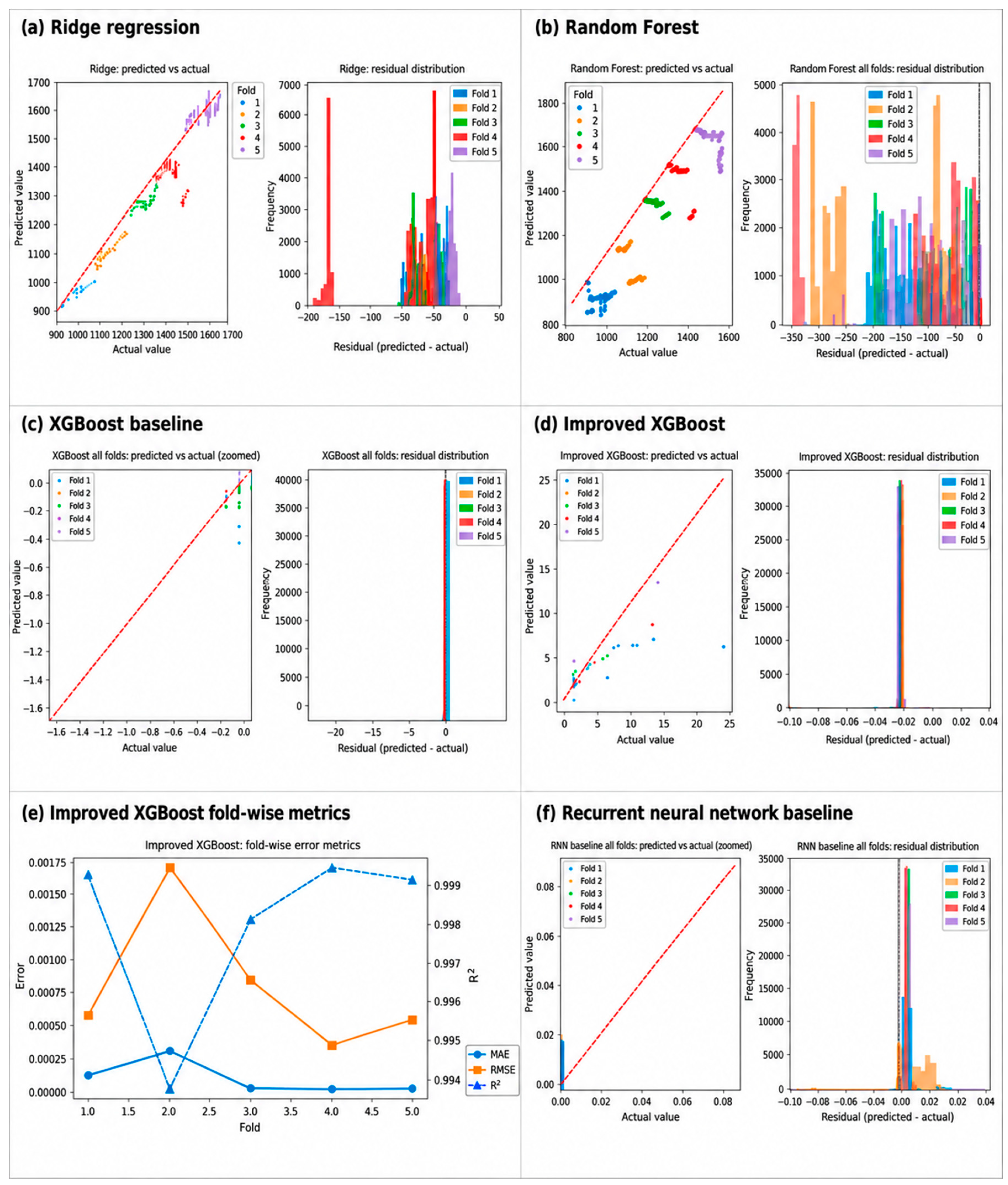
Figure 4: Overview of Single-Model validation results. Note: (a) ridge regression; (b) random forest; (c) baseline XGBoost; (d) improved XGBoost; (e) fold-wise metric changes of improved XGBoost; (f) recurrent neural network baseline.
Based on the single-model validation, this study further compares the overall performance of different modeling schemes under the same dataset and differential prediction target. It should be noted that the models share the same data source, main preprocessing workflow, and evaluation metrics, but their input feature forms and use of temporal information are not completely identical. Therefore, the results in this section are mainly used to explain the adaptability differences of different modeling schemes on the current dataset, rather than to provide a pure algorithm ranking under strictly controlled feature inputs.
In terms of average evaluation metrics, the models exhibit clear performance stratification, as shown in Fig. 5. Ridge regression provides a linear reference but has limited ability to explain nonlinear fluctuations in differential energy consumption. Random Forest introduces nonlinear tree structures but does not obtain a stable advantage, indicating that static ensemble trees are sensitive to low-variance test windows and local spikes. Baseline XGBoost substantially improves over the linear model and ordinary tree model, showing that the gradient-boosting framework is more suitable for this type of differential target. Improved XGBoost performs best in MAE, RMSE, and R2, indicating that robust target processing, multi-scale time-series features, and regularized training strategies can improve model adaptability to sparse spike sequences. Although the recurrent neural network baseline uses sequence inputs, it does not show a comprehensive advantage when near-zero samples dominate and spike samples are limited.
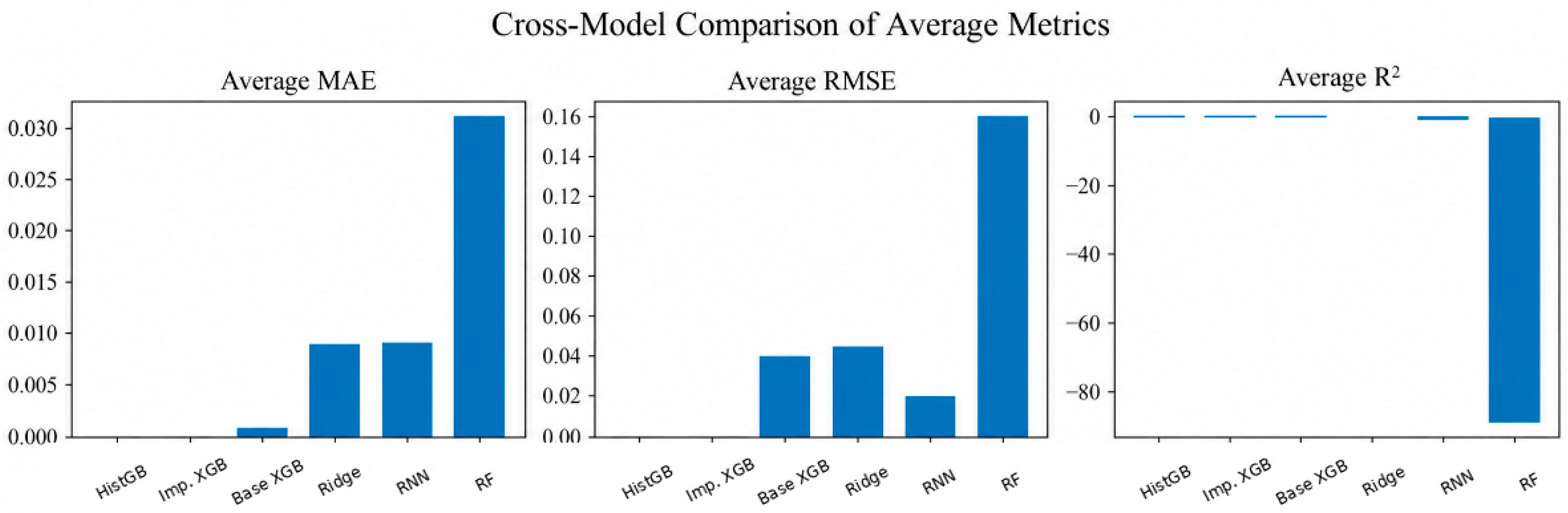
Figure 5: Comparison of average evaluation metrics across models.
The figure shows the average performance of each validation model in terms of MAE, RMSE, and R2. Lower MAE and RMSE indicate smaller errors, while higher R2 indicates stronger explanatory power.
In terms of cross-fold stability, as shown in Fig. 6, Ridge regression has relatively high overall error, Random Forest shows large fold-to-fold fluctuations, baseline XGBoost achieves some error convergence, and improved XGBoost maintains low MAE in most folds. This suggests that its advantage is reflected not only in average metrics but also in stability across changing time windows. The recurrent neural network baseline does not show extreme error divergence, but its overall explanatory power remains insufficient, further indicating that explicit sequence input is not necessarily suitable for highly sparse differential targets.
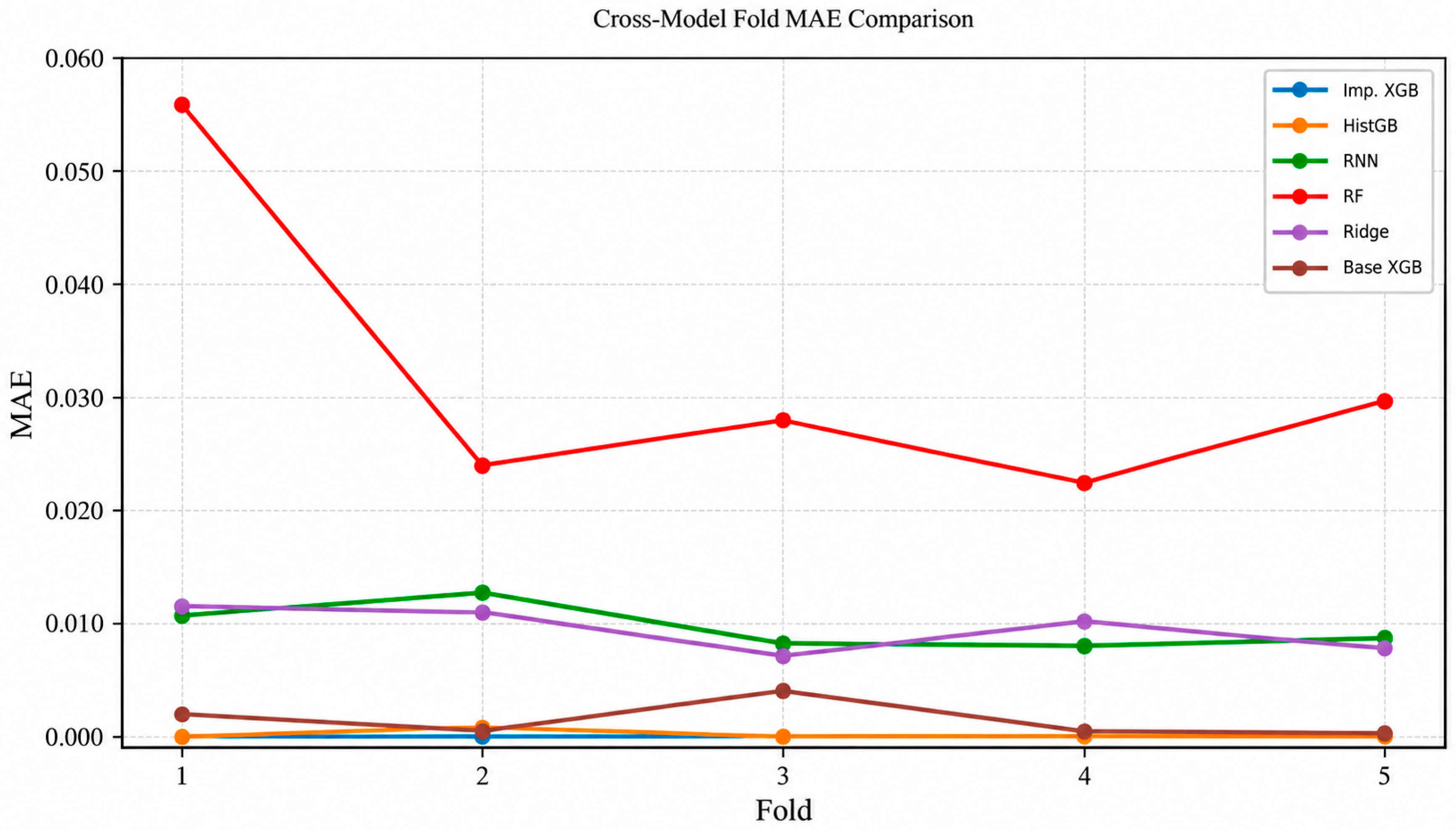
Figure 6: Fold-Wise MAE comparison across models.
The figure shows the MAE changes of each model under five-fold validation and is used to observe prediction stability across different time windows.
Overall, performance improvements in controlled environmental chamber differential energy consumption prediction depend not only on model complexity, but also on whether target processing, feature representation, and training strategies match the data structure. Because the cross-model comparison is still affected by differences in input features, this paper further sets up a unified feature-input experiment to compare the basic ability of different models to use the same feature information.
4.4 Model Capability Comparison under Unified Feature Inputs
To further assess the influence of input-feature differences on the cross-model comparison, this study adds an experiment with unified feature inputs. The input range is limited to indoor temperature, indoor humidity, indoor dew point, indoor CO2 concentration, indoor illuminance, outdoor temperature, one-record lag, 24-record lag, five-record rolling mean, 24-record rolling mean, hour, weekday, and weekend indicator. Ridge regression, Random Forest, baseline XGBoost, and the recurrent neural network baseline are compared under the same differential energy consumption target and five-fold time-series validation protocol. It should be noted that the recurrent neural network still uses sliding-window inputs due to its structure, but the variable sources are kept consistent with the other models. Therefore, this experiment is mainly used to compare the basic capability of different models to use the same feature information.
Table 10 shows that, under unified feature-input conditions, the performance differences between models narrow substantially. The MAE values of Ridge regression and RNN/GRU-LSTM are close, while Random Forest and baseline XGBoost do not show stable advantages. This indicates that, without sufficient feature engineering and robust training strategies, model structure alone is not enough to stably improve differential energy consumption prediction accuracy.
Table 10: Prediction performance of different models under unified feature inputs.
| Model | MAE | RMSE | R2 | SMAPE (%) |
|---|---|---|---|---|
| Ridge regression | 0.009215 ± 0.001198 | 0.021560 ± 0.001606 | −0.023057 ± 0.046523 | 198.93 ± 0.20 |
| Random forest | 0.012741 ± 0.004894 | 0.023277 ± 0.003353 | −0.194317 ± 0.229889 | 197.92 ± 1.07 |
| XGBoost (baseline) | 0.011119 ± 0.003538 | 0.022196 ± 0.002371 | −0.084334 ± 0.129339 | 198.13 ± 0.92 |
| RNN/GRU-LSTM | 0.008775 ± 0.000996 | 0.021344 ± 0.001124 | −0.003649 ± 0.002252 | 199.13 ± 0.21 |
In terms of R2, all four models are close to zero or slightly negative, suggesting that the low variance, high sparsity, and local spike structure of differential energy consumption limit the models’ ability to explain overall variance. Therefore, the advantage of the improved XGBoost in the previous sections should not be attributed simply to the model type. It should instead be understood as the combined effect of robust target processing, multi-scale time-series features, rolling statistics, and regularized training strategies.
4.5 XGBoost Feature Ablation Experiment
To analyze the contribution of different feature types to XGBoost prediction performance, this study conducts a feature ablation experiment while keeping the model type, prediction target, evaluation metrics, and five-fold time-series partitioning fixed. Four groups are designed with gradually increasing feature information: Group A uses only the original environmental variables; Group B adds one-record lag and 24-record lag; Group C further adds five-record rolling mean and 24-record rolling mean; and Group D further adds time-derived variables including hour, weekday, and weekend indicator.
Table 11 shows that XGBoost already has a certain level of error control when using only the original environmental variables. After one-record lag and 24-record lag are added, MAE and R2 do not improve substantially, indicating that the marginal contribution of single-point lag information is limited for the current highly sparse differential target. After five-record rolling mean and 24-record rolling mean are further added, MAE decreases to 0.010386 ± 0.002266 and R2 improves from −0.040287 to −0.016571, suggesting that rolling statistics are more helpful for representing local operating states and the short-window background of energy consumption changes.
Table 11: Results of the XGBoost feature ablation experiment.
| Experiment Group | Feature Configuration | MAE | RMSE | R2 |
|---|---|---|---|---|
| A | Original environmental variables | 0.010965 ± 0.002078 | 0.021985 ± 0.001551 | −0.038144 ± 0.039473 |
| B | A + lag1 + lag24 | 0.010998 ± 0.002431 | 0.022010 ± 0.001702 | −0.040287 ± 0.053715 |
| C | B + rolling5 + rolling24 | 0.010386 ± 0.002266 | 0.021757 ± 0.001620 | −0.016571 ± 0.045541 |
| D | C + hour + weekday + weekend indicator | 0.010730 ± 0.002919 | 0.022021 ± 0.001882 | −0.041256 ± 0.075139 |
After time-derived variables are further added in Group D, MAE rises to 0.010730 ± 0.002919 and R2 does not further improve, indicating that time-derived variables such as hour, weekday, and weekend indicator have limited marginal benefits in the current dataset. As shown in Fig. 7, XGBoost prediction performance does not improve monotonically as the number of features increases. Group C performs relatively best, suggesting that rolling statistical features are the feature type with the clearest contribution in this ablation experiment.
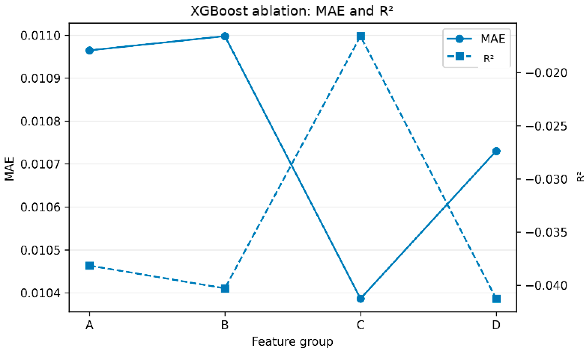
Figure 7: Changes in MAE and R2 in the XGBoost feature ablation experiment.
Fig. 7 further shows that XGBoost prediction performance does not improve monotonically with increasing feature quantity. Among the four groups, Group C performs relatively best, indicating that five-record rolling mean and 24-record rolling mean are the most clearly beneficial feature types in this ablation experiment. This result supports the inclusion of multi-scale rolling statistics in the improved XGBoost model and also shows that model performance improvement depends on the match between feature construction and the structure of differential energy consumption data.
In summary, the ablation experiment shows that the performance improvement of the improved XGBoost mainly relies on the match between differential target processing, local rolling statistical features, training stability control, and the data structure.
4.6 Traditional Time-Series Baseline and Simple Baseline Models
To assess whether complex models provide clear advantages over basic prediction rules, this study introduces three baseline methods: ARIMA, Historical mean, and Naive last. ARIMA serves as a traditional univariate time-series reference, Historical mean represents a global mean-prediction baseline, and Naive last tests the short-term persistence of differential energy consumption. All three baselines follow the same data protocol as the main models, including differential energy construction from cumulative electricity readings, negative-difference removal, and P99.5 percentile truncation.
ARIMA uses only the historical differential energy consumption series, without indoor or outdoor environmental variables. Since the modeling target is already differential energy consumption, d is set to 0, and the order is selected from ARIMA (1, 0, 0), ARIMA (2, 0, 0), ARIMA (1, 0, 1), ARIMA (2, 0, 1), and ARIMA (2, 0, 2) using AIC/BIC. In five-fold validation, ARIMA (2, 0, 2) is selected in most folds, achieving MAE, RMSE, and R2 values of 0.009649 ± 0.000784, 0.021184 ± 0.001095, and 0.010924 ± 0.003160, respectively. This suggests that the target series contains limited short-term correlation, but historical target values alone provide only modest predictive improvement.
Historical mean obtains MAE, RMSE, and R2 values of 0.009779 ± 0.000786, 0.021318 ± 0.001111, and −0.001573 ± 0.001513, respectively, reflecting the performance of a static mean baseline. Naive last achieves a slightly lower MAE of 0.009504 ± 0.001083, but its RMSE increases to 0.030789 ± 0.001731 and its R2 decreases to −1.088521 ± 0.017048. This indicates that the single-step persistence rule can capture local inertia but is more sensitive to spikes, rapid declines, and operating-state transitions. The average evaluation metrics of the three baseline models are compared in Fig. 8.
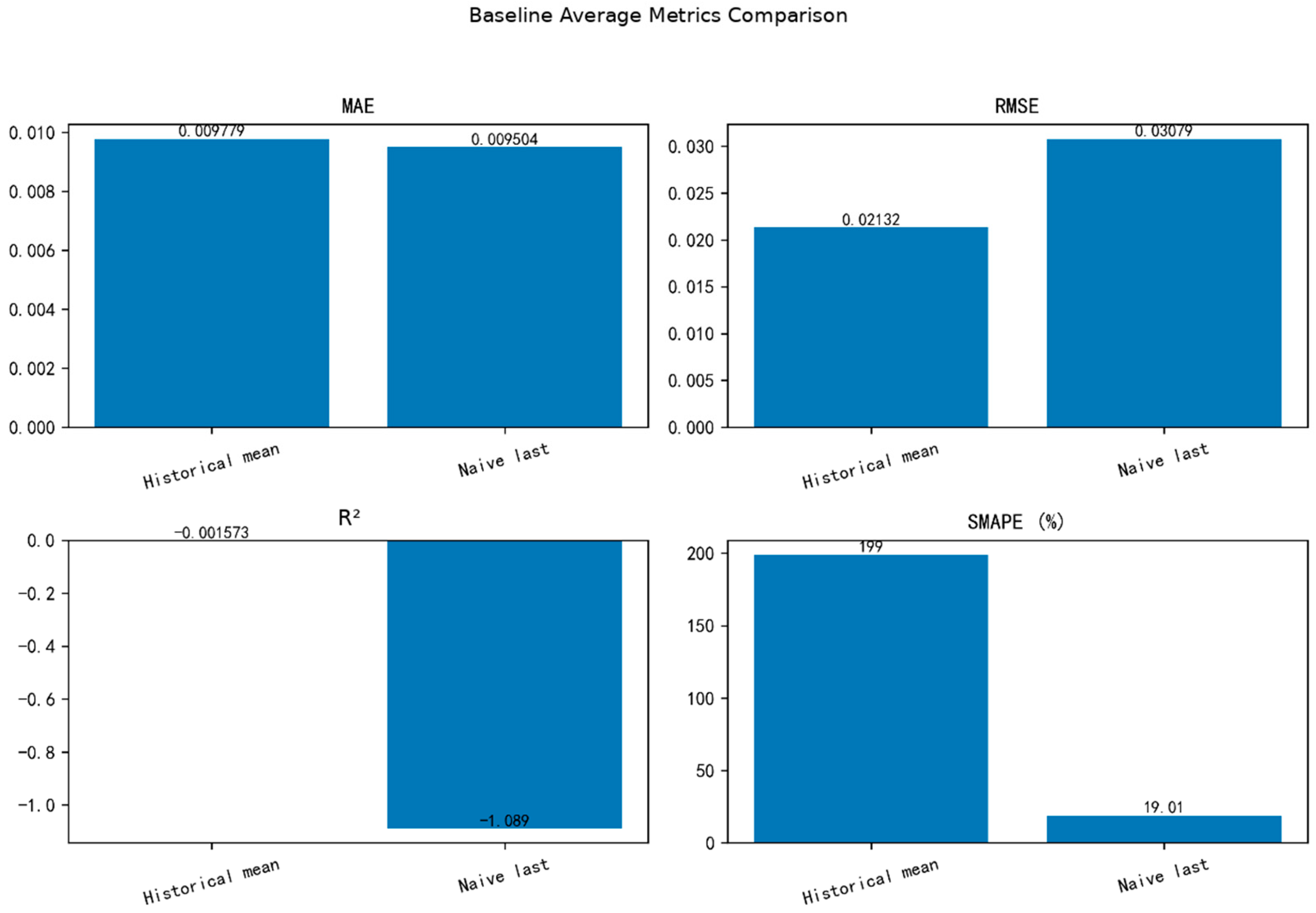
Figure 8: Comparison of average evaluation metrics for simple baseline models.
In terms of fold-to-fold stability, Historical mean is relatively smooth, Naive last fluctuates more strongly, and the MAE and RMSE of ARIMA are close to those of Historical mean, while its R2 is slightly above zero. This indicates that the traditional univariate time-series model can use part of the historical correlation, but has difficulty representing environmental disturbances, local spikes, and equipment-state changes. Because SMAPE for the three baselines is strongly affected by many zero or near-zero samples, this study still uses MAE, RMSE, and R2 as the main criteria. The five-fold MAE changes of the baseline models are further shown in Fig. 9.
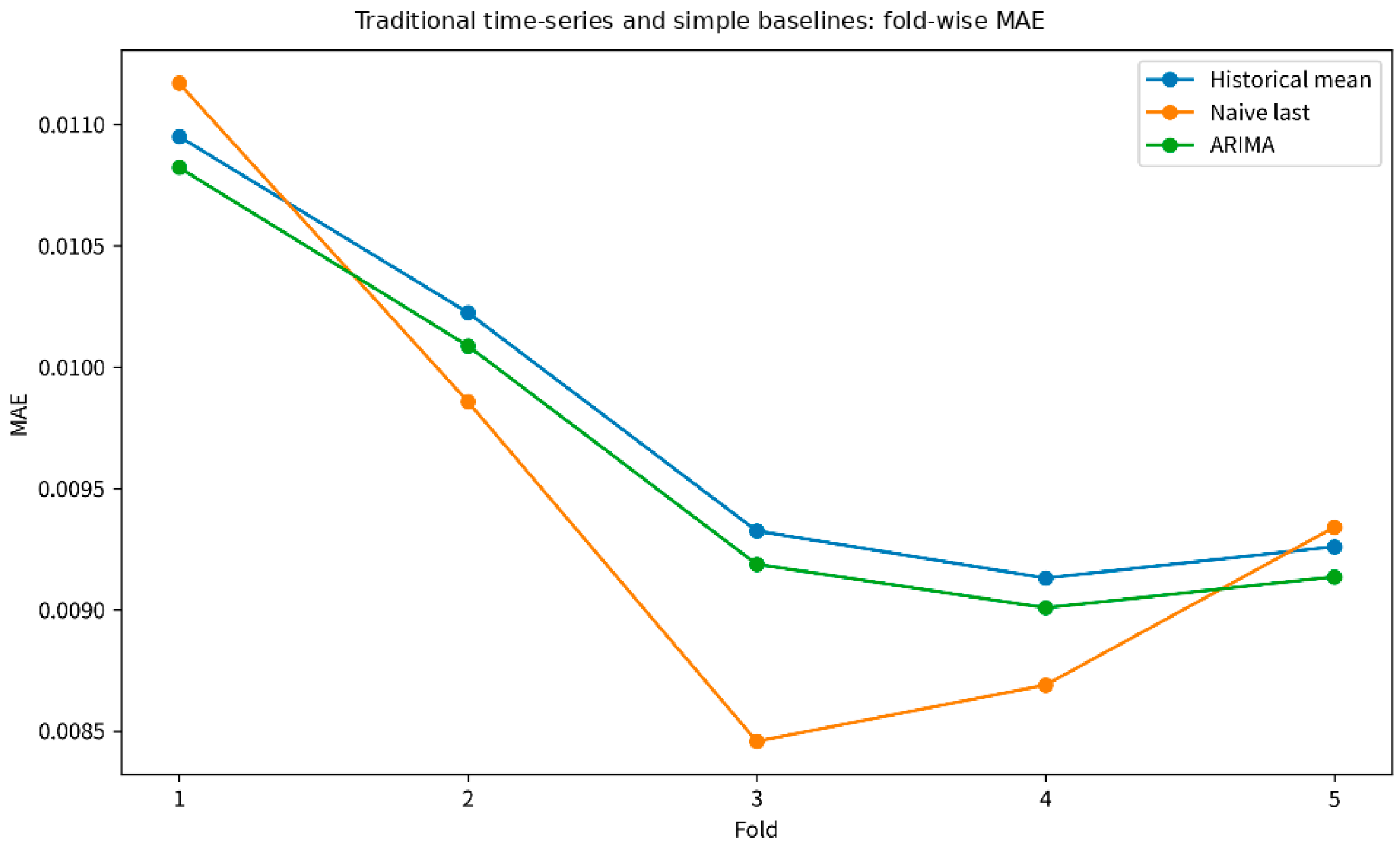
Figure 9: Five-Fold MAE changes of the simple baseline models.
Overall, Historical mean, Naive last, and ARIMA provide global mean, single-step inertia, and traditional univariate time-series modeling references, respectively. None of the three uses external environmental variables or complex feature engineering, so they mainly serve as minimum comparable baselines rather than as final model-selection candidates.
The principal model-specific results for Historical mean, Naive last, ARIMA, Ridge regression, Random Forest, baseline XGBoost, improved XGBoost, and the recurrent neural network baseline are summarized in Table 12.
Table 12: Summary of main prediction results for all models.
| Model | MAE | RMSE | R2 | SMAPE (%) | Result Positioning |
|---|---|---|---|---|---|
| Historical mean | 0.0098 ± 0.0008 | 0.0213 ± 0.0011 | −0.0016 ± 0.0015 | 198.96 ± 0.17 | Global mean baseline |
| Naive last | 0.0095 ± 0.0011 | 0.0308 ± 0.0017 | −1.0885 ± 0.0170 | 19.01 ± 2.17 | Short-term inertia baseline |
| ARIMA | 0.0096 ± 0.0008 | 0.0212 ± 0.0011 | 0.0109 ± 0.0032 | 197.67 ± 0.60 | Traditional univariate time-series baseline |
| Ridge regression | 0.0094 ± 0.0019 | 0.0423 ± 0.0206 | 0.2605 ± 0.0160 | 194.35 ± 0.40 | Linear reference model |
| Random forest | 0.0321 ± 0.0138 | 0.1615 ± 0.2096 | −93.2433 ± 206.9260 | 195.90 ± 1.03 | Static nonlinear tree model with insufficient cross-fold stability |
| XGBoost (baseline) | 0.0013 ± 0.0016 | 0.0385 ± 0.0472 | 0.7834 ± 0.2049 | 158.63 ± 10.44 | Baseline gradient-boosted tree model |
| Improved XGBoost workflow | 0.0001 ± 0.0001 | 0.0008 ± 0.0005 | 0.9981 ± 0.0025 | 114.57 ± 50.61 | Best result within the model-specific comparison |
| Recurrent neural network baseline | 0.0096 ± 0.0020 | 0.0212 ± 0.0015 | −0.0342 ± 0.0498 | 198.96 ± 0.42 | Recurrent neural network baseline with insufficient overall advantage |
Table 12 presents the model-specific comparison reported in Section 4.1, Section 4.2, Section 4.3, Section 4.4, Section 4.5, Section 4.6 and Section 4.7. In contrast, the additional analyses in Section 4.8, Section 4.9, Section 4.10 and Section 4.11 adopt a more conservative expanding-window evaluation protocol, in which target capping is determined separately within each fold, while lag, rolling and non-zero-window features are constructed strictly from historical observations.
Table 12 shows that Historical mean, Naive last, and ARIMA form three baseline references. Historical mean reflects the global mean-prediction level. Naive last can use short-term inertia but is sensitive to spikes and rapid declines, resulting in poor RMSE and R2 performance. The MAE and RMSE of ARIMA are close to those of Historical mean, but its R2 is slightly above zero, indicating that the differential energy consumption series itself has a certain short-term correlation structure. Because ARIMA uses only historical target-series values and cannot use environmental variables or multi-scale time-series features, its overall improvement is limited.
Compared with the baseline models, Ridge regression provides a linear reference but is insufficient for representing nonlinear coupling and local spikes. Random Forest has nonlinear representation capability but shows large fold-to-fold fluctuations. Baseline XGBoost substantially improves over the linear model and ordinary tree model, indicating that the gradient-boosting framework is more suitable for the complex error structure in differential energy consumption. The improved XGBoost workflow further combines robust differential target processing, P99.5 percentile truncation, multi-order lag features, rolling statistics, non-zero-window features, time-derived variables, regularization, and early stopping, and achieves better results in MAE, RMSE, and R2.
Although the recurrent neural network baseline uses sliding-window sequence inputs, it tends to produce smoothed predictions under a target distribution with high sparsity and a large proportion of near-zero samples, and does not show a comprehensive advantage over boosted tree models. Overall, the key to differential energy consumption prediction for controlled environmental chambers is not simply increasing model complexity, but ensuring that target processing, time-series feature representation, and training strategies match the data structure. This requirement is also consistent with studies of cold-storage facilities, controlled-environment optimization, and refrigerated-system load prediction, in which energy behavior is linked to environmental and operating conditions [18,19,21]. The dataset can support prediction tests using traditional time-series models, machine learning models, and neural network models, and can also reveal differences in the adaptability of different modeling paradigms under sparsity, spike fluctuations, and short-term temporal dependence.
4.8 Temporal Transfer and Forecast-Horizon Analysis
An expanding-window evaluation was applied to successive test months from the same chamber. The May, June and July MAE values were 0.01825, 0.01628 and 0.01428 kWh per valid record transition, and the corresponding RMSE values were 0.02948, 0.02688 and 0.02569 kWh per valid record transition. From May to July, MAE and RMSE decreased by 21.8% and 12.9%, respectively, while R2 changed from −0.0273 to 0.0813. These results indicate improved later-period prediction as the training history expanded within the observed chamber. (Fig. 10).
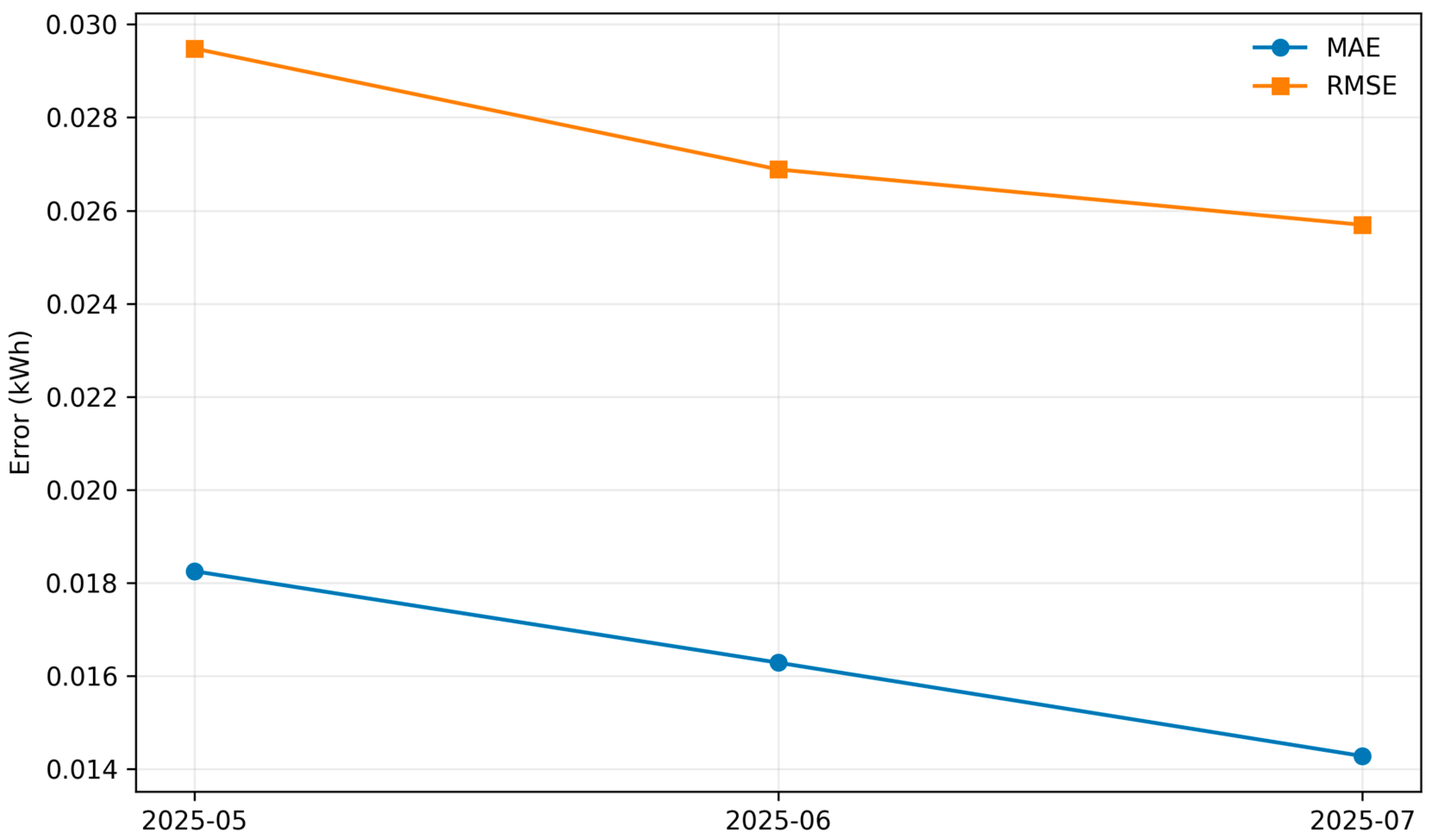
Figure 10: Expanding-Window performance by test month.
Across the observed outdoor-temperature, absolute temperature-gap and relative-humidity groups, RMSE ranged from 0.02646 to 0.02731 kWh, 0.02443 to 0.02855 kWh and 0.02564 to 0.02675 kWh, respectively, showing comparable error levels across the recorded operating conditions. For direct forecasts at 1, 5, 15, 30 and 60 record steps, RMSE values were 0.02743, 0.02730, 0.02880, 0.02824 and 0.02992 kWh per valid record transition; the change from 1 to 60 record steps was approximately 9.1%. In contrast, 60-record-step cumulative-energy RMSE reached 0.43900 kWh (Fig. 11). The results support short-horizon use and periodic model updating.
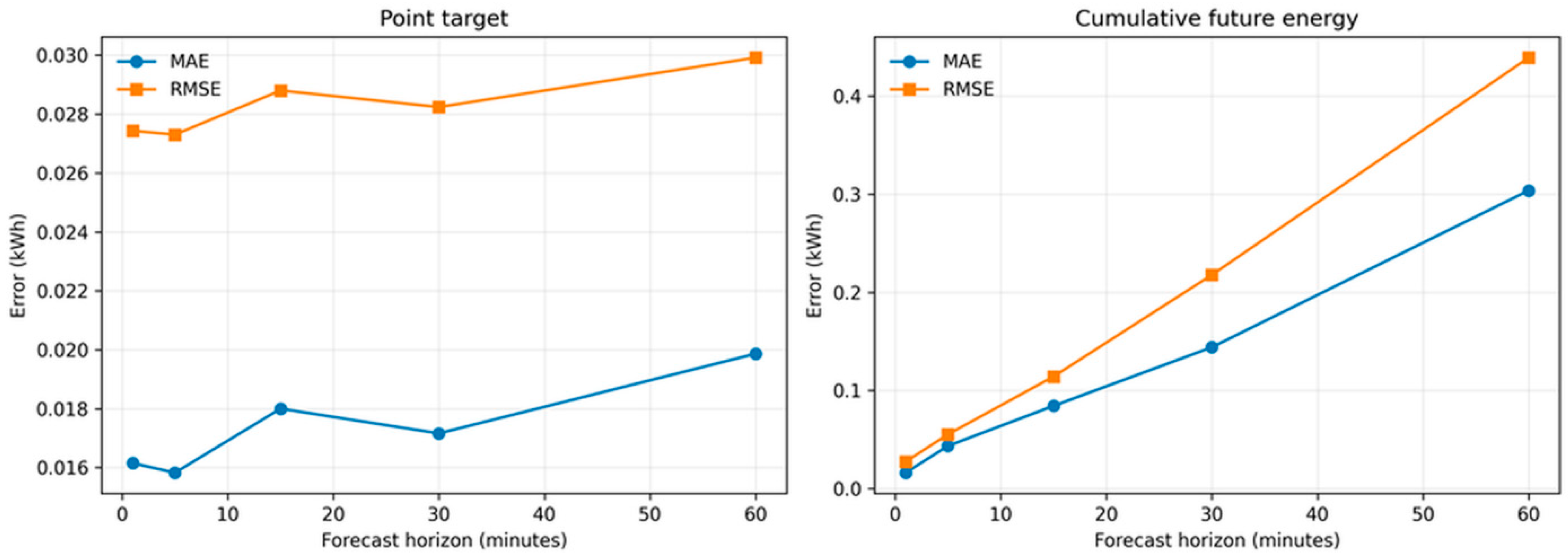
Figure 11: Direct Multi-Step and Cumulative-Energy prediction.
One-factor-at-a-time tests examined target capping, history windows, tree depth, learning rate, and column sampling. P99, P99.5, and P99.9 produced the same 0.1 kWh-per-transition threshold because of the discrete increment distribution, whereas removing the cap slightly increased RMSE to 0.02674 kWh per valid record transition. The default history configuration performed best among the tested windows; max_depth = 5 remained preferable, learning rates from 0.02 to 0.08 were stable, and colsample_bytree = 0.6 produced the lowest error in its comparison (Fig. 12). The results support the selected settings within the tested ranges rather than implying a universal optimum.
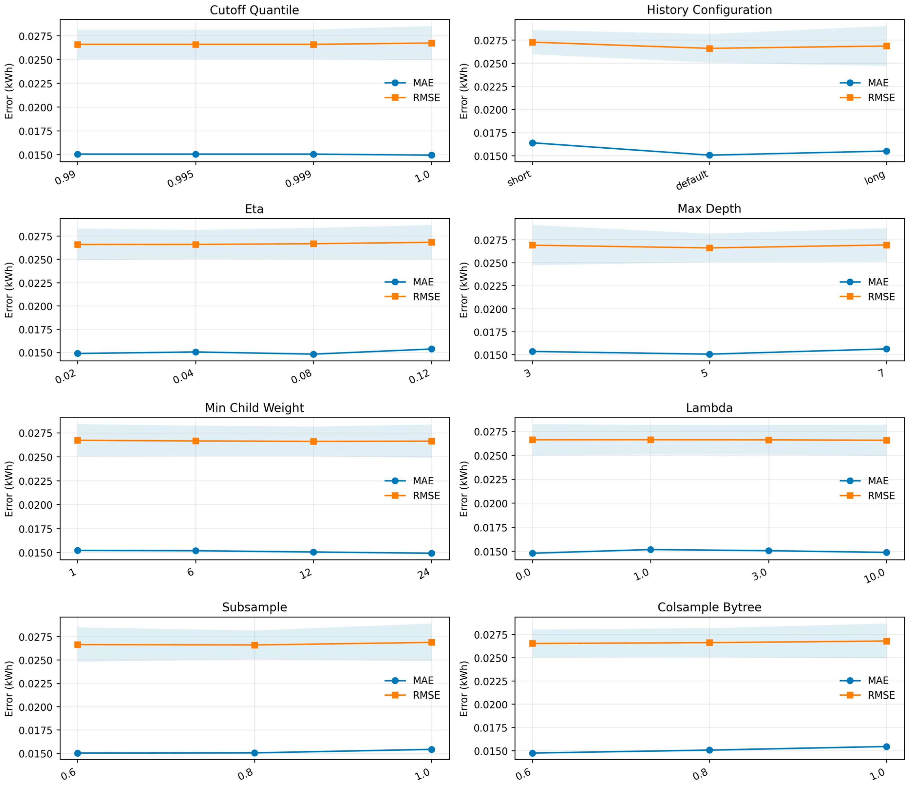
Figure 12: XGBoost parameter sensitivity.
4.10 Feature Importance and High-Increment Events
Fold-aggregated importance scores were calculated for XGBoost and Random Forest. For XGBoost, the five-record non-zero count (0.1659), five-record rolling mean (0.1608) and indoor illuminance (0.1022) ranked highest. For Random Forest, indoor temperature (0.1756), indoor illuminance (0.1727) and indoor humidity (0.1106) were the leading variables. The rankings show that historical sparse-event patterns and environmental states provide complementary model-specific information; importance values are interpreted as predictive associations (Fig. 13).
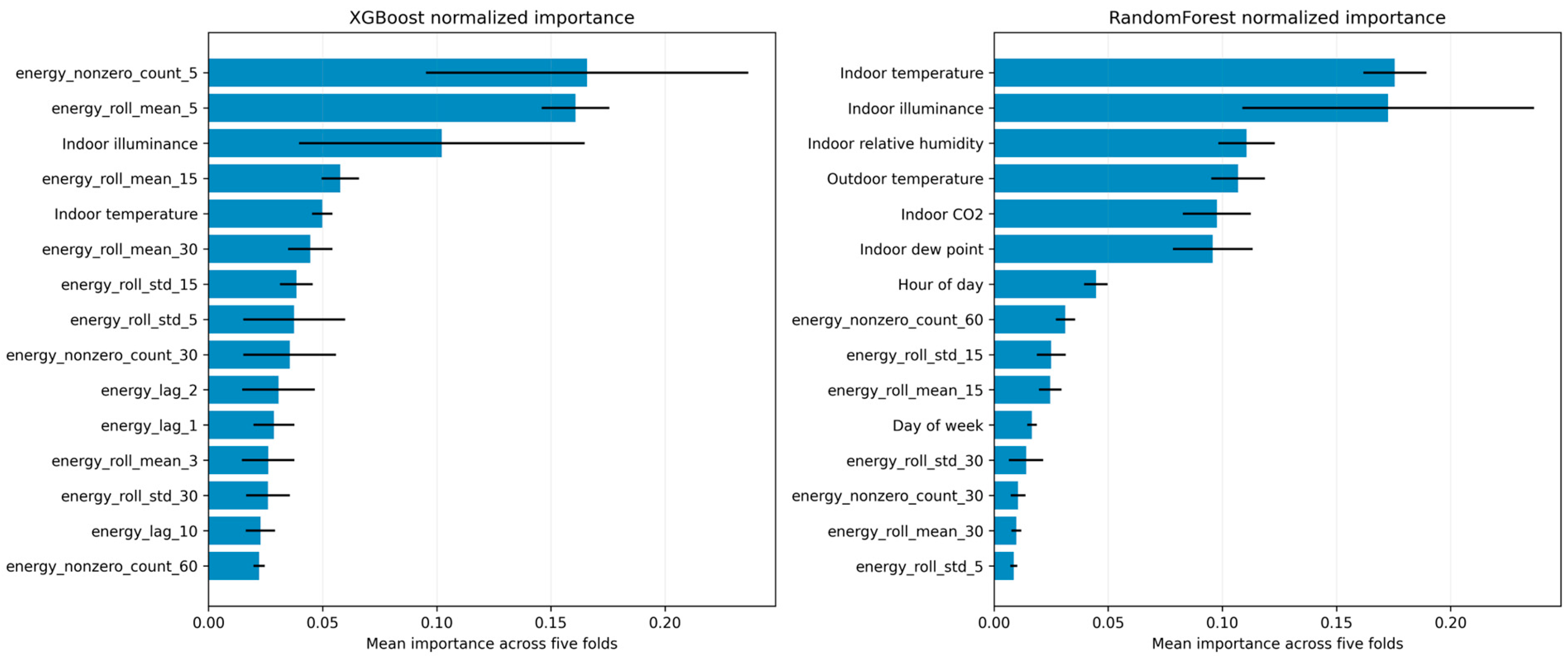
Figure 13: Feature importance with Fold-to-Fold variability.
The uncapped raw series contained 31 successive-record increments of 0.2 kWh. Three mutually separated events with complete ±30-record windows were examined to characterize synchronous environmental changes around these increments (Fig. 14). The synchronized patterns show that high-increment events coincide with distinct changes in the monitored environmental conditions, supporting an operational interpretation of the feature-importance results. These event-level observations are therefore discussed as predictive and temporal associations within the chamber monitoring framework.
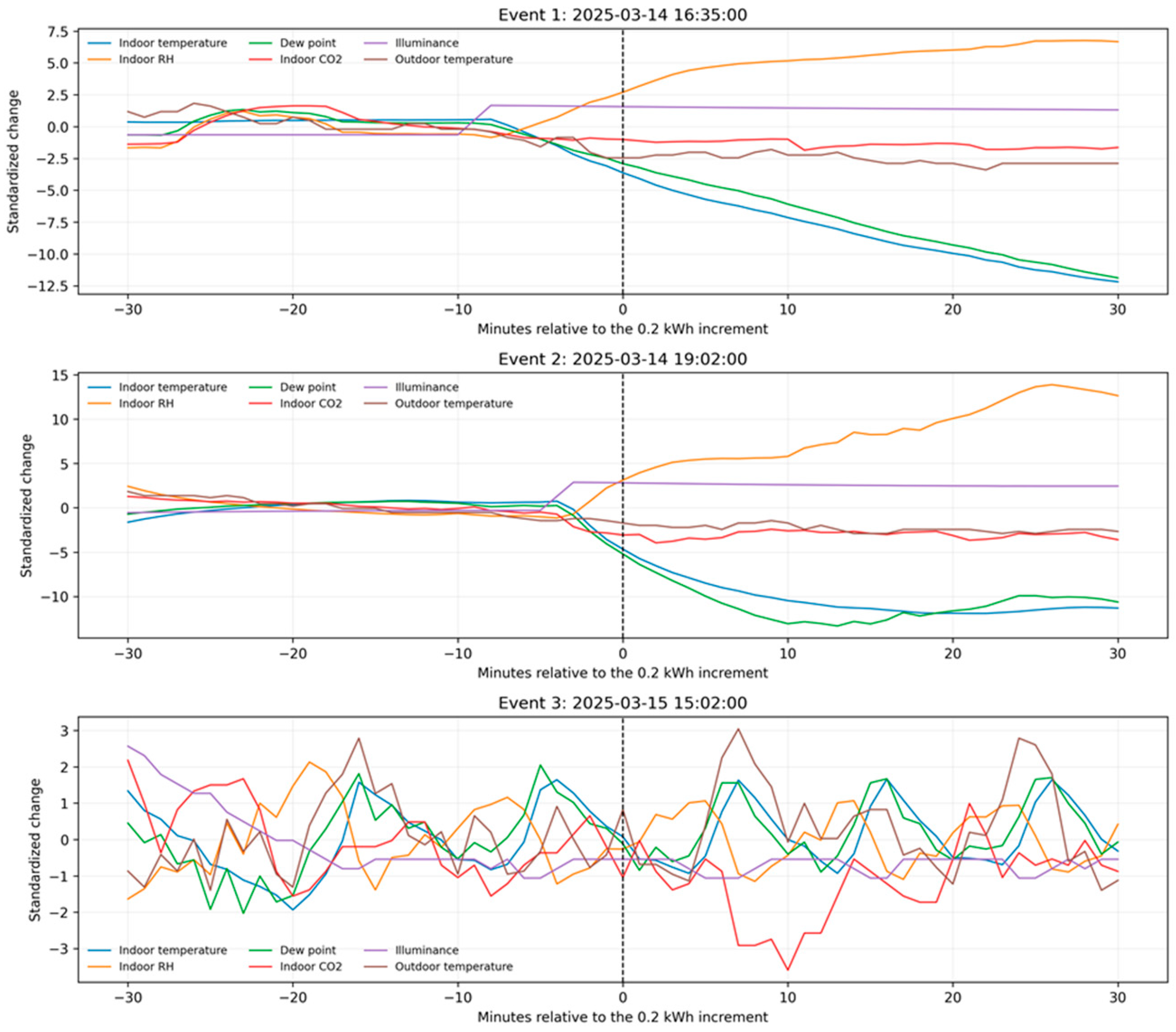
Figure 14: Environmental variables around selected High-Increment events.
4.11 Derived Physical-Feature Ablation
Eleven sensor-derived variables were added to the environmental, historical, and calendar inputs: signed and absolute indoor–outdoor temperature gaps, dew-point depression, vapor-pressure deficit, absolute humidity, CO2 excess above 400 ppm, and five successive-record sensor changes. Under the stricter expanding-window configuration used for the fold-matched ablation, mean MAE decreased from 0.01464 to 0.01215 kWh per valid record transition (17.00%), mean RMSE decreased from 0.02655 to 0.02421 kWh per valid record transition (8.82%), and mean R2 increased from 0.0634 to 0.2216 (Fig. 15). Although the absolute R2 remained modest, the simultaneous improvement in all three metrics indicates that the sensor-derived physical features provide complementary predictive information. These results further show that physically interpretable thermal, moisture, air-quality, and dynamic-response descriptors can enhance the representation of chamber operating conditions under the conservative evaluation protocol.
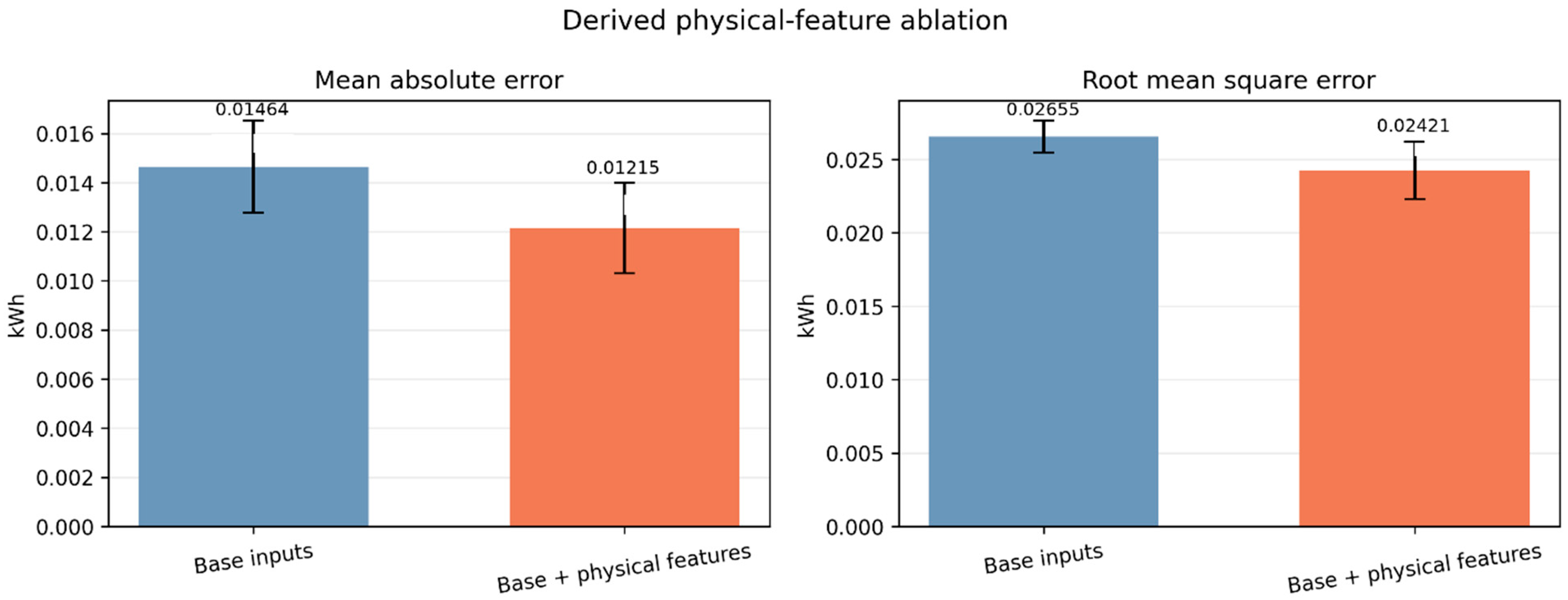
Figure 15: Paired ablation of Sensor-Derived physical features.
This study developed a data-driven workflow for short-term differential energy consumption forecasting in a controlled environmental chamber. The improved XGBoost workflow achieved the best performance in the model-specific comparison, while the unified-feature and ablation analyses showed that robust target processing, time-series feature construction, and sensor-derived physical features contribute to prediction performance. Under the expanding-window protocol, the addition of physical features reduced mean MAE by 17.00% and RMSE by 8.82%. Overall, the proposed workflow provides a practical basis for short-horizon energy monitoring, anomaly screening, load management, and low-carbon operation. Future work may further extend the proposed framework toward broader operating scenarios and control-oriented energy management applications.
Acknowledgement:
Funding Statement: This work was supported by the 2026 General Research Project of the China Society of Logistics and China Federation of Logistics & Purchasing (2026CSLKT3-433).
Author Contributions: Bowen Yuan: conceptualization, methodology, software, data curation, formal analysis, validation, visualization, and writing—original draft. Huwei Liu: methodology, validation, supervision, and writing—review & editing. Jingyun Liu: resources, funding acquisition, project administration, supervision, and writing—review & editing. Yuchen Lin: validation, visualization, and writing—review & editing. All authors reviewed and approved the final version of the manuscript.
Availability of Data and Materials: The data that support the findings of this study are available from the corresponding author upon reasonable request. The raw operational data are not publicly available due to laboratory data management restrictions.
Ethics Approval: Not applicable.
Conflicts of Interest: The authors declare no conflicts of interest.
Supplementary Materials: The following supporting information is available online: Table S1: Hyperparameters and training settings of the prediction models. The supplementary material is available online at https://www.techscience.com/doi/10.32604/ee.2026.088401/s1.
Abbreviations
The following abbreviations are used in this manuscript:
| ACF | Autocorrelation function |
| ADF | Augmented Dickey–Fuller test |
| AIC | Akaike information criterion |
| ARIMA | Autoregressive integrated moving average |
| BIC | Bayesian information criterion |
| CO2 | Carbon dioxide concentration |
| CSV | Comma-separated values |
| GRU | Gated recurrent unit |
| HVAC | Heating, ventilation and air conditioning |
| KNN | k-nearest neighbors |
| KPSS | Kwiatkowski–Phillips–Schmidt–Shin test |
| LSTM | Long short-term memory |
| MAE | Mean absolute error |
| PACF | Partial autocorrelation function |
| PLC-HMI | Programmable logic controller and human-machine interface |
| RMSE | Root mean square error |
| RNN | Recurrent neural network |
| SMAPE | Symmetric mean absolute percentage error |
| XGBoost | Extreme gradient boosting |
References
1. Amasyali K , El-Gohary NM . A review of data-driven building energy consumption prediction studies. Renew Sustain Energy Rev. 2018; 81: 1192– 205. doi:10.1016/j.rser.2017.04.095. [Google Scholar] [CrossRef]
2. Sarbu I , Adam M . Experimental and numerical investigations of the energy efficiency of conventional air conditioning systems in cooling mode and comfort assurance in office buildings. Energy Build. 2014; 85: 45– 58. doi:10.1016/j.enbuild.2014.09.022. [Google Scholar] [CrossRef]
3. Wang G , Song L . Air handling unit supply air temperature optimal control during economizer cycles. Energy Build. 2012; 49: 310– 6. doi:10.1016/j.enbuild.2012.02.024. [Google Scholar] [CrossRef]
4. Soyguder S , Karakose M , Alli H . Design and simulation of self-tuning PID-type fuzzy adaptive control for an expert HVAC system. Expert Syst Appl. 2009; 36( 3): 4566– 73. doi:10.1016/j.eswa.2008.05.031. [Google Scholar] [CrossRef]
5. Bahramnia P , Rostami SMH , Wang J , Kim GJ . Modeling and controlling of temperature and humidity in building heating, ventilating, and air conditioning system using model predictive control. Energies. 2019; 12( 24): 4805. doi:10.3390/EN12244805. [Google Scholar] [CrossRef]
6. Volkaerts D , Youssef A , Ozcan SE , Exadaktylos V , Bleyaert P , Berckmans D . Modelling greenhouse temperature and humidity in order to develop an energy-saving model-based control strategy. Commun Agric Appl Biol Sci. 2011; 76( 1): 37– 40. [Google Scholar]
7. Touzani S , Granderson J , Fernandes S . Gradient boosting machine for modeling the energy consumption of commercial buildings. Energy Build. 2018; 158: 1533– 43. doi:10.1016/j.enbuild.2017.11.039. [Google Scholar] [CrossRef]
8. Fan C , Xiao F , Zhao Y , Wang J . Analytical investigation of autoencoder-based methods for unsupervised anomaly detection in building energy data. Appl Energy. 2018; 211: 1123– 35. doi:10.1016/j.apenergy.2017.12.005. [Google Scholar] [CrossRef]
9. Zhao HX , Magoulès F . A review on the prediction of building energy consumption. Renew Sustain Energy Rev. 2012; 16( 6): 3586– 92. doi:10.1016/j.rser.2012.02.049. [Google Scholar] [CrossRef]
10. Bourdeau M , Zhai XQ , Nefzaoui E , Guo X , Chatellier P . Modeling and forecasting building energy consumption: a review of data-driven techniques. Sustain Cities Soc. 2019; 48: 101533. doi:10.1016/j.scs.2019.101533. [Google Scholar] [CrossRef]
11. Wang T , Pan YQ , Huang ZZ . Application of gradient boosted regression trees in short-term building energy consumption prediction. Build Energy Effic. 2018; 46( 3): 112– 6. (In Chinese). doi:10.3969/j.issn.1673-7237.2018.03.024. [Google Scholar] [CrossRef]
12. Tso GKF , Yau KKW . Predicting electricity energy consumption: a comparison of regression analysis, decision tree and neural networks. Energy. 2007; 32( 9): 1761– 8. doi:10.1016/j.energy.2006.11.010. [Google Scholar] [CrossRef]
13. Cui Z , Cao Y , Wu G , Liu H , Qiu Z , Chen C . Research on preprocessing technology of building energy consumption monitoring data based on machine learning algorithm. Build Sci. 2018; 34( 2): 94– 9. (In Chinese). doi:10.13614/j.cnki.11-1962/tu.2018.02.15. [Google Scholar] [CrossRef]
14. Xiao Z , Gang W , Yuan J , Chen Z , Li J , Wang X , et al. Impacts of data preprocessing and selection on energy consumption prediction model of HVAC systems based on deep learning. Energy Build. 2022; 258: 111832. doi:10.1016/j.enbuild.2022.111832. [Google Scholar] [CrossRef]
15. Zhang L , Wen J , Li Y , Chen J , Ye Y , Fu Y , et al. A review of machine learning in building load prediction. Appl Energy. 2021; 285: 116452. doi:10.1016/j.apenergy.2021.116452. [Google Scholar] [CrossRef]
16. Türkmen AC , Januschowski T , Wang Y , Cemgil AT . Forecasting intermittent and sparse time series: a unified probabilistic framework via deep renewal processes. PLoS One. 2021; 16( 11): e0259764. doi:10.1371/journal.pone.0259764. [Google Scholar] [CrossRef]
17. Jeon Y , Seong S . Robust recurrent network model for intermittent time-series forecasting. Int J Forecast. 2022; 38( 4): 1415– 25. doi:10.1016/j.ijforecast.2021.07.004. [Google Scholar] [CrossRef]
18. Alkhulaifi N , Bowler AL , Pekaslan D , Serdaroglu G , Closs S , Watson NJ , et al. Machine learning pipeline for energy and environmental prediction in cold storage facilities. IEEE Access. 2024; 12: 153935– 51. doi:10.1109/ACCESS.2024.3482572. [Google Scholar] [CrossRef]
19. Chen WH , Mattson NS , You F . Intelligent control and energy optimization in controlled environment agriculture via nonlinear model predictive control of semi-closed greenhouse. Appl Energy. 2022; 320: 119334. doi:10.1016/j.apenergy.2022.119334. [Google Scholar] [CrossRef]
20. Wang Y , Chen J , Cao B , Liu X , Zhang X . Energy consumption prediction of cold storage based on LSTM with parameter optimization. Int J Refrig. 2025; 175: 12– 24. doi:10.1016/j.ijrefrig.2025.03.033. [Google Scholar] [CrossRef]
21. Rasoulinezhad E . Green Taxes innovation and energy imports in advancing renewable transitions in developing countries. Resour Policy. 2025; 102: 105517. doi:10.1016/j.resourpol.2025.105517. [Google Scholar] [CrossRef]
Cite This Article
 Copyright © 2026 The Author(s). Published by Tech Science Press.
This work is licensed under a Creative Commons Attribution 4.0 International License , which permits unrestricted use, distribution, and reproduction in any medium, provided the original work is properly cited.
 Downloads
 Citation Tools
