Predictive Maintenance Strategy for Photovoltaic Power Systems: Collaborative Optimization of Transformer-Based Lifetime Prediction and Opposition-Based Learning HHO Algorithm

1  Introduction

In recent years, the scale of photovoltaic (PV) power generation has been growing rapidly, and effective operation and maintenance of PV power generation systems is essential to ensure their reliability and economy during operation. Usually, maintenance approaches for PV power generation systems are broadly classified into three forms: corrective maintenance (CM), preventive maintenance (PM), and predictive maintenance (PdM) [1–3].

The CM strategy for PV systems involves emergency repairs to restore operation after a system failure. Reference [4] established a general economic evaluation model and found that when the response time of the maintenance team is short, the CM strategy often has the lowest total cost in most scenarios, particularly suitable for small-scale PV plants with fewer components. Reference [5] decomposed the CM process into failure and repair processes and proposed an automated aggregation algorithm to model the failure and repair processes of multiple components in complex systems, simplifying the computational burden of CM modeling.

The PM strategy for PV systems involves performing maintenance before failures occur, primarily by establishing specific maintenance cycles for regular maintenance activities to minimize downtime caused by component failures and reduce unnecessary economic losses. Reference [6] established a preventive maintenance model for photovoltaic power generation systems based on reliability, and used the Zebra optimization algorithm to determine the maintenance threshold. Reference [7] proposed a refined fault detection method based on current signal analysis as a key support for improving PM accuracy, aiding in triggering PM at early fault stages to extend component lifespan and enhance system availability. Reference [8] proposed a preventive maintenance and replacement strategy for photovoltaic power generation systems based on reliability constraints. It constructed a non-periodic incomplete maintenance model and determined the optimal maintenance and replacement cycle by combining the inverter case study. Reference [9] proposed a PM strategy driven by structural correlation for PV systems, aiming to reduce high costs due to unreasonable maintenance timing and grouping. Reference [10] constructed a reliability model and a maintenance cost model for the wind-solar hybrid power system. By combining preventive maintenance and energy complementation strategies, it established a maintenance optimization model and verified its effectiveness through a case study.

The PdM strategy for PV systems is condition-based maintenance, involving periodic or continuous condition monitoring and fault diagnosis of key components during system operation, with maintenance performed when necessary [11]. Reference [12] focused on the three core tasks of condition monitoring, fault diagnosis, and lifespan prediction, summarizing common signal types, fault modes, and degradation features, and analyzing the application scenarios and adaptability of deep learning models in PdM. Reference [13] proposed a PdM optimization method for distributed PV plants by constructing a multi-constraint scheduling model and introducing genetic algorithms to achieve dynamic allocation of maintenance tasks guided by fault levels, equipment capacity, and remaining waiting time. Reference [14] addressed the challenge of predicting PV component degradation under dynamic environmental conditions, proposing a semi-parametric PdM framework that explicitly incorporates environmental condition information into Remaining Useful Life (RUL) prediction models, demonstrating effective support for PdM decisions in various PV technologies for health management and fault prevention. Reference [15] constructed a method for predicting the lifespan of photovoltaic modules and optimizing maintenance based on a two-stage Wiener degradation model. It proposed a predictive maintenance strategy to determine the optimal maintenance threshold and timing. Reference [16] proposed a data-driven process based on machine learning and time series methods for the performance modeling, fault detection, and trend prediction of photovoltaic systems, thereby achieving predictive maintenance alerts. Reference [17] provides a comprehensive review of predictive maintenance and fault diagnosis methods based on artificial intelligence in photovoltaic systems, and proposes a framework that combines fault mode analysis and severity assessment to enhance system reliability and operational efficiency.

In summary, the CM strategy of PV power generation system mainly takes whether the system is intact or whether it can continue to be used as the basis of maintenance, and restores the equipment to the initial state through repair or replacement actions after failure, which is a typical unplanned maintenance strategy, which will definitely lead to problems such as long downtime, large losses, and poor safety, and is not applicable to systems with high safety and reliability requirements; the PM strategy performs better in cost optimization compared to CM strategy, but in most cases, the optimal maintenance interval needs to be found, which poses a challenge to the actual operation. Building on the foregoing analysis, this study introduces a PdM framework for PV power systems that leverages RUL information. First, a Transformer network forecasts the system’s RUL. Second, the predicted RUL values are coupled with an operation-and-maintenance (O&M) cost formulation, and an opposition-based-learning Harris Hawks Optimization (OHHO) algorithm simultaneously adjusts the maintenance threshold L and restoration factor r. Thereby deriving an optimal maintenance schedule. Finally, through simulation, it was verified that this model can utilize the degraded data of the photovoltaic power generation system to predict its RUL, and this strategy can effectively reduce the total maintenance cost and enhance the forward-looking nature of maintenance decisions, thereby effectively extending the remaining useful life of the system.

2  RUL Prediction Model for Photovoltaic Power Generation Systems

2.1 Transformer Model

The Transformer architecture leverages a self-attention mechanism for sequence modelling. It comprises an encoder and a decoder built by stacking identical layers; each layer contains a multi-head attention block and a position-wise feed-forward network, supplemented with residual connections and layer normalization modules [18]. The overall structure of the Transformer is shown schematically in Fig. 1.

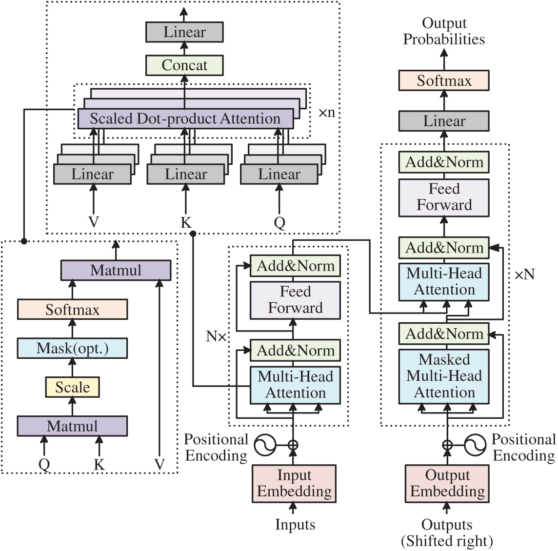
Figure 1: Schematic diagram of the overall structure of Transformer

In the illustration, the encoder is placed on the left and the decoder on the right; within both, multi-head attention blocks and position-wise feed-forward networks are linked through residual paths and followed by layer-normalization. The zoomed-in image in the upper left of the figure demonstrates the computation of multi-head attention: the inputs are linearly transformed to produce queries (Q), keys (K), and values (V), which are spliced through multiple parallel sets of scaled dot-product attentions and linearly mapped to obtain the final output.

Self-attention is the pivotal operation within the Transformer architecture and is realised through scaled dot-product attention. Let the query, key and value matrices be denoted by Q, K and V, respectively. The computation proceeds as follows: (i) calculate the dot-product similarity between each query and every key, (ii) divide these scores by the square root of the key-vector dimension, (iii) convert the scaled scores into probability weights via the Softmax function, and (iv) obtain the output as the probability-weighted sum of the value vectors. The corresponding expression is:

Attention(Q,K,V)=softmax(QKTdk)V(1)

In the equation, dk represents the dimension of the key vectors. The expression details the self-attention workflow: for each query, dot-product scores against every key are first calculated, then divided by dk and normalised through the Softmax function, producing a probability distribution over the keys. These coefficients weight the associated value vectors, whose weighted combination forms the layer’s output. Through this operation, self-attention fuses contextual cues from all positions in the input, effectively modelling long-range dependencies. Multi-head attention enhances the mechanism by mapping Q, K and V into n distinct representation subspaces that are processed in parallel. For the i-th head, let the transformed query, key, and value be denoted as QWiQ, KWiK, and VWiV, respectively. Attention is computed separately in each subspace, and the resulting outputs are concatenated:

headi=Attention(QWiQ,KWiK,VWiV)(2)

Multihead(Q,K,V)=Con(head1,…,headn)WO(3)

Through multi-head parallelism, the model can focus on sequence features from different perspectives, enhancing its expressive capability. The Transformer also requires explicit injection of positional information because self-attention itself cannot distinguish the order of elements in a sequence. A widely used technique introduces periodic positional signals into the token embeddings by superimposing sine-and cosine-based vectors. For a token located at position pos and a model dimension index i, the corresponding positional component is given by:

PE(pos,2i)=sin⁡(pos100002i/dm)(4)

PE(pos,2i+1)=cos⁡(pos100002i/dm)(5)

In the formula, dm is the model dimension, with even indices using the sine function and odd indices using the cosine function, ensuring that encodings for adjacent positions have different frequencies, which allows sequences of varying lengths to be distinguished. The positional encoding is added to the input embeddings and serves as the input to the self-attention module, conveying the positional arrangement of elements within the token stream. The above derivations ensure that the Transformer model can perform parallel computations while effectively representing relationships and positional information between elements when processing sequence data.

2.2 RUL Prediction Model of PV Power System Based on Transformer Model

Focusing on the degradation characteristics of PV power-system data, a Transformer-based model is constructed to predict the RUL. Firstly, the power degradation data collected during system operation is regarded as time series input. In order to be compatible with the input form of Transformer, the original features need to be mapped to a fixed-dimension vector space through linear layers, and position coding is added to reflect the time sequence. The architecture centres on a stack of Transformer encoder layers; every layer pairs a multi-head self-attention module with a position-wise fully connected network, and employs residual links together with layer normalization to keep training stable. The top-layer encoder output is passed through a dense regression layer, which converts it into remaining-lifetime estimates for forecasting future service life. The input sequence is first transformed through embedding and positional encoding, then fed into an N-layer Transformer encoder stack—each layer comprising a multi-head self-attention block and a position-wise feed-forward network—and finally passed through a dense regression head to yield the system’s remaining-lifetime prediction [19].

During training, the raw degradation data are first segmented and perturbed to emulate fragmentary input sequences. Parameter updates are driven by minimizing the mean-squared error (MSE). For a dataset containing N samples, let yi denote the actual lifetime of the i-th instance and yi′, its predicted counterpart; the loss is then given by the MSE formulation:

LMSE=1N∑i=1N(yi′−yi)2(6)

By gently penalising prediction deviations—yet assigning greater weight to large errors—the loss guides the regression task toward robust convergence of its parameter updates. The optimization process continuously adjusts the model parameters through the gradient descent method to minimize the MSE loss and thus improve the prediction accuracy.

3  Predictive Maintenance Model for PV Power System Based on RUL Information

For a photovoltaic power generation system structured as shown in Fig. 2, perform maintenance on its associated system.

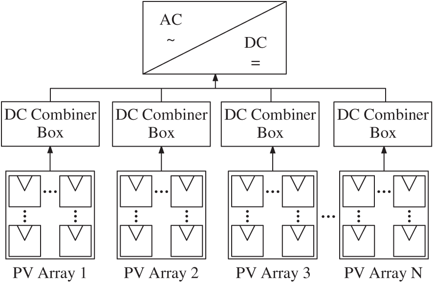
Figure 2: Structure diagram of PV power generation system

3.1 CM Strategy Model and PM Strategy Model

Under the CM strategy, the system operates continuously until a failure occurs, at which point maintenance is performed. The cost per renewal cycle is the failure repair cost, CC, and the renewal cycle is the system lifespan T [20]. Therefore, the expected cost and expected cycle are as follows:

E(C)=CC(7)

E(T)=∫0∞R(t)dt(8)

In this expression, R(t) denotes the survival function—that is, the likelihood that the system remains operational up to time t. The cost rate of the CM strategy is then given by:

CCM=E(C)E(T)=CC∫0∞R(t)dt(9)

For the PM strategy, assume the maintenance cycle is τ. At the start of each cycle, if a failure occurs before τ with probability F(τ), maintenance is performed at the time of failure, incurring a cost of CC, and the cycle length is the failure time. If the system has not failed by τ, with probability R(τ)=1−F(τ), a planned maintenance is performed at τ, incurring a cost of CP, and the cycle length is τ. According to renewal theory [21], the expected cost and expected cycle length for periodic maintenance can be expressed as:

E(C)=CPR(τ)+CC[1−R(τ)](10)

E(T)=∫0τR(t)dt(11)

Therefore, the cost rate of the PM strategy is:

CPM=E(C)E(T)=CPR(τ)+CC[1−R(τ)]∫0τR(t)dt(12)

3.2 Predictive Maintenance Model for Photovoltaic Power Generation System Based on RUL Information

The PdM strategy for the photovoltaic power generation system utilizes the real-time assessed TRUL, setting a maintenance threshold L and a recovery factor r (0≤r≤1). Maintenance is performed when the predicted remaining useful life TRUL≤L. The degree of recovery after maintenance depends on r. If the original lifespan is T, and T>L, preventive maintenance is performed at t=L, with the time remaining until failure given by:

Δ=T−L+rL=T−(1−r)L(13)

The total operating time is L+Δ=T+rL. Fig. 3 illustrates the complete maintenance workflow.

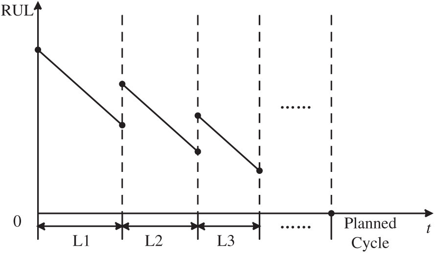
Figure 3: Schematic diagram of the maintenance process

If a failure occurs before the maintenance threshold—denoted as case T≤L—with a probability of F(L), then the cycle length is T and the cycle cost is CC. If the maintenance threshold is triggered before failure—denoted as case T>L—with a probability of 1−F(L), then the cycle length is T−(1−r)L and the cycle cost is CC+CP. Based on these two scenarios, The PdM strategy’s expected cost and cycle duration can be formulated as:

E(C)=CCF(L)+(CP+CC)[1−F(L)](14)

E(T)=∫0Ltf(t)dt+∫L∞[t−(1−r)L]f(t)dt(15)

Accordingly, the cost rate for the PdM strategy is defined as:

CPdM=E(C)E(T)=CCF(L)+(CP+CC)[1−F(L)]∫0Ltf(t)dt+∫L¥[t−(1−r)L]f(t)dt(16)

In the actual solution, if the distribution of T is known, the above integrals can be calculated numerically directly; if the distribution is unknown or difficult to analyze, Monte Carlo simulation can be used, and then approximate calculation. It is worth noting that the above cost analysis did not include the monitoring costs for a specific period of time, and this aspect needs to be given special consideration in practical applications.

3.3 Solving Optimal Maintenance Strategy for PV Power System Based on OHHO

3.3.1 Opposition-Based-Learning Harris Hawks Optimization

Harris Hawks Optimization (HHO) is a swarm-based meta-heuristic that models the cooperative encirclement tactics observed in Harris’s hawks [22]. HHO balances broad exploration with intensive exploitation by emulating the encirclement tactics Harris’s hawks use to corner prey within the search space, and its basic process includes an exploration phase, a transition phase, and an exploitation phase [23].

(1) Exploratory stage

This stage consists of two strategies:

X⁡(t+1)={Xr⁡(t)−r1⁢|Xr−2⁢r2⁢X⁡(t)|Δ⁢X−r3⁢(L⁢B+r4⁢Δ⁢B)⁢q≥0.5q<0.5(17)

where X(t+1) denotes the eagle’s location in the upcoming iteration, Xi represents the current coordinates of the prey, X(t) denotes the eagle’s present location, Xr(t) corresponds to an eagle chosen at random from the present swarm, r1, r2, r3, r4, q are all sampled at random within the range (0, 1), which will be updated as iteration proceeds, ΔB=UB−LB, UB and LB are the upper and lower bounds of the variables, respectively, ΔX=Xi(t)−Xm(t), and Xm(t) indicates the mean location of all eagles in the present swarm, as defined below:

Xm=1N∑i=1NXi(t)(18)

where Xi(t) represents the location of an eagle at iteration t, and N is the population size.

(2) Transition stage

The escape energy of prey at this stage is modeled as follows:

E=2E0(1−tT)(19)

where E is the escape energy of the prey, T is the maximum number of iterations, t is the current number of iterations, and E0 is the initial energy, which takes the value of a random number within (−1, 1). When |E|≥1, the Harris hawk will search different regions to further explore the location of the prey—global exploration; when |E|<1, the Harris hawk enters into local exploration.

(3) Development phase

Let the escape probability of the prey be R. According to the values of E and R, the following four roundup strategies can be set up:

The soft roundup—|E|≥0.5, R≥0.5, is modeled by the following rule:

X(t+1)=ΔX(t)−E|JXi(t)−X(t)|(20)

ΔX(t)=Xi(t)−X(t)(21)

where ΔX(t) is the difference between the position vector of the prey in the t-th iteration and the current position vector, and the value of J varies randomly during the iteration, characterizing the fleeing intensity of the prey.

The results of the hard roundup—|E|<0.5, R≥0.5, position update are as follows:

X(t+1)=Xi(t)−E|ΔX(t)|(22)

Indirect fast dive soft roundups—|E|≥0.5, R<0.5, are executed by the following maneuvers:

Y=Xi(t)−E|JXi(t)−X(t)|(23)

Z=Y+S×LF(D)(24)

where D is the problem dimension, S is a random vector, and LF is the Lévy flight function, defined as follows:

{LF(x)=0.01×u×σ|μ|1βσ=(Γ(1+β)×sin⁡(πβ2)Γ(1+β2)×β×2β−12)1β(25)

where u, μ are random values within (0, 1) and β is a default constant. Therefore, the position of this phase is updated as follows:

X⁡(t+1)={Y,Z,⁢F⁡(Y)<F⁡(X⁡(t))F⁡(Z)<F⁡(X⁡(t))(26)

Indirect fast dive hard roundups—|E|<0.5, R<0.5, are executed by the following maneuvers:

Y=Xi(t)−E|JXi(t)−Xm(t)|(27)

Z=Y+S×LF(D)(28)

where Xm is obtained from Eq. (18). Therefore, the position of this stage is updated as follows:

X⁡(t+1)={Y,Z,⁢F⁡(Y)<F⁡(X⁡(t))F⁡(Z)<F⁡(X⁡(t))(29)

However, HHO may converge slowly and easily fall into local optimum when dealing with complex optimization problems. To enhance algorithmic performance, an opposition-based learning (OBL) mechanism is incorporated into OHHO, aiming to boost search efficiency and maintain population diversity [24], which accelerates the current solution by considering both the current solution and its opposites simultaneously to convergence and extend the search space by considering both the current solution and its opposites. Specifically, given a range of values for the j-th dimension in the decision variable space [aj,bj], for a current solution Xoppi=(xi1opp,xi2opp,…,xiDopp), its corresponding inverse solution is defined as:

xijopp=aj+bj−xij,j=1,2,…,D(30)

where D is the problem dimension. This reverse mapping makes the reverse solution located at the symmetric position of the current solution relative to the center of the hypercube, with an exploration direction relative to the original solution. After generating the reverse individuals, the current population is evaluated for fitness together with its reverse population, and a reverse selection strategy is used to construct a new generation of populations optimally. A common practice is to compare the fitness values f(Xi) and f(Xoppi) for each individual Xi. If the reverse solution is superior, Xoppi is substituted for Xi, otherwise the original solution is retained:

Xnewi={Xoppi,f(Xoppi)<f(Xi)Xi,otherwise(31)

Through the aforementioned reverse selection mechanism, it can help the algorithm escape from local extreme points, thereby accurately and efficiently determining the optimal combination of maintenance threshold and recovery factor required.

3.3.2 Model Solving

The model solving process is shown in Fig. 4, and the main steps are as follows:

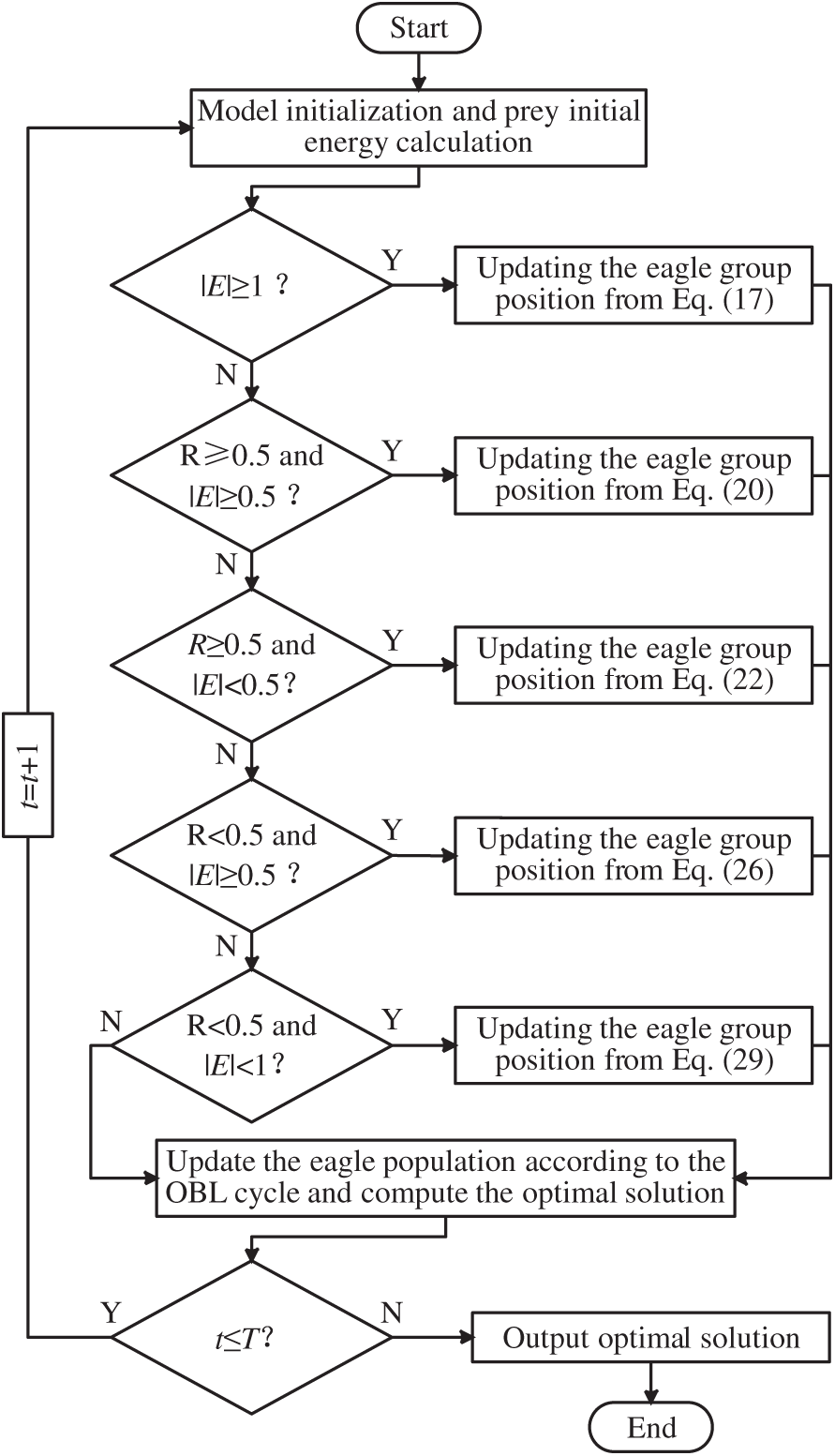
Figure 4: Model solution process

Step 1: Parameter initialization. Set the algorithm parameters—the population size N, the maximum number of iterations T, and the periodic reverse operation interval K. Randomly generate N candidate solutions, each individual containing the parameter vector Xi=(Li,ri), and compute their corresponding reverse solutions Xoppi, respectively:

Loppi=Lmin+Lmax−Li(32)

roppi=rmin+rmax−ri(33)

where L is the repair threshold and r is the recovery factor. The fitness is evaluated for all original and reversed individuals, and each (L, r) is substituted into the system predictive maintenance model to calculate the corresponding objective function value. The 2N candidate solutions are ranked according to the fitness values, and the top N solutions are optimally retained to form the initial population, providing a better starting point for the iterative process.

Step 2: Global iteration update. Let the current iteration number t = 1. In each iteration, first calculate the prey’s escape energy En and escape probability R, and then determine whether it is currently in the exploration phase or exploitation phase. For each eagle group individual Xti=(Li,ri), update its position according to the following: in the exploration phase, update the individual according to HHO’s stochastic exploration formula; in the exploitation phase, execute different roundup strategies according to the escape probability R. Execute soft roundup when R≥0.5, otherwise execute hard roundup, and compute d against different formulas Xt+1i. Calculate the fitness for all the new individuals again after the update, and write down the current optimal solution Xbest.

Step 3: Periodic reverse operation. If the current number of iterations satisfies the conditions of reverse operation, perform reverse learning again for the whole population updated in step 2, generate a reverse solution for each individual, and evaluate its fitness. The current population is merged with the reverse population and sorted by fitness, and the top N individuals are optimally selected as the new population. This step allows the algorithm to periodically introduce symmetric exploration nodes in the search space, which helps to update the population diversity and accelerate global convergence.

Step 4: Termination judgment. For the iteration number t, if t≤T, then return to step 2 to continue the iteration; otherwise, the iteration is terminated and the currently recorded optimal solution Xbest is output as the optimal configuration of the predictive maintenance parameters L and r. The maintenance strategy corresponding to this optimal solution is the optimal combination of maintenance parameters for the system under the given fault and degradation conditions.

3.4 The Overall Framework of the Model

Based on the above analysis, Fig. 5 presents the flowchart of the maintenance decision-making process described in this paper, covering the entire process from RUL prediction to the formulation of system maintenance decisions based on RUL information. In the RUL prediction stage, the proposed model’s prediction model can learn the degradation pattern of the equipment and use the fragment data to predict the system’s RUL. During the stage of formulating the equipment maintenance strategy, the proposed PdM strategy monitors the RUL information of the photovoltaic power generation system in real time and finds the lowest annual cost rate through OHHO. Moreover, the convergence performance of this algorithm is superior to that of HHO.

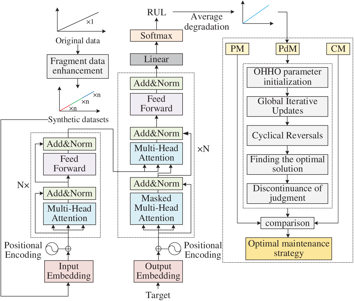
Figure 5: Flowchart of the model process

4  Case Analysis

The PdM strategy for the PV power system analyzes the power degradation process of a 5.28 kW system based on 22 PV modules over a period of 12.5 a, as shown in Fig. 6. This system consists of 2 sets of PV strings connected in parallel, while each string consists of 11 PV modules connected in series [25].

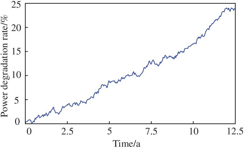
Figure 6: Power degradation process of photovoltaic system

4.1 RUL Analysis of PV Power Systems with Fragmented Data

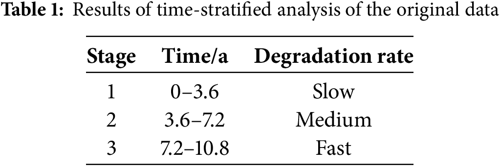
According to the overall process of this study, firstly, the overall degraded data is stratified. Based on the expected service life of the system in the case where no maintenance decisions are made, it is divided into three stages as shown in Table 1.

Next, in order to simulate the output power degradation rate of the system under different working environments, data augmentation was carried out based on the initial power degradation curve. 200 different degradation curves were generated for each segment. By adding random weak perturbations to each segment, the power degradation rate fluctuated within the range of 10% above and below the initial value. This achieved the enhancement of the original data. The results of data augmentation are shown in Fig. 7. The introduced weak perturbations can bolster the prediction model’s resistance to observed disturbances without altering the system’s overall degradation trajectory.

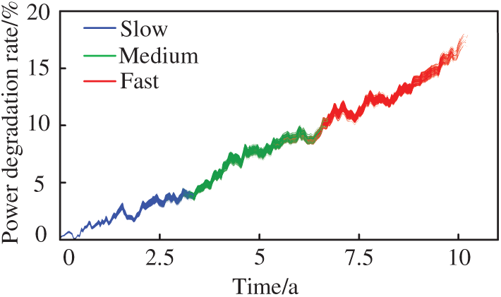
Figure 7: Result of degraded data enhancement

The results of degradation data augmentation can be used as the original dataset for the system’s RUL prediction. For the augmented data under different degradation rates, 80% of each set is selected as the training set and 20% as the test set. The Transformer model is utilized to achieve the training of the training set data, and the training process is shown in Fig. 8.

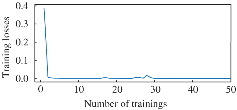
Figure 8: Training process of the Transformer model

Subsequently, the data from the test set was utilized for the prediction of the system RUL, and the prediction results are shown in Fig. 9.

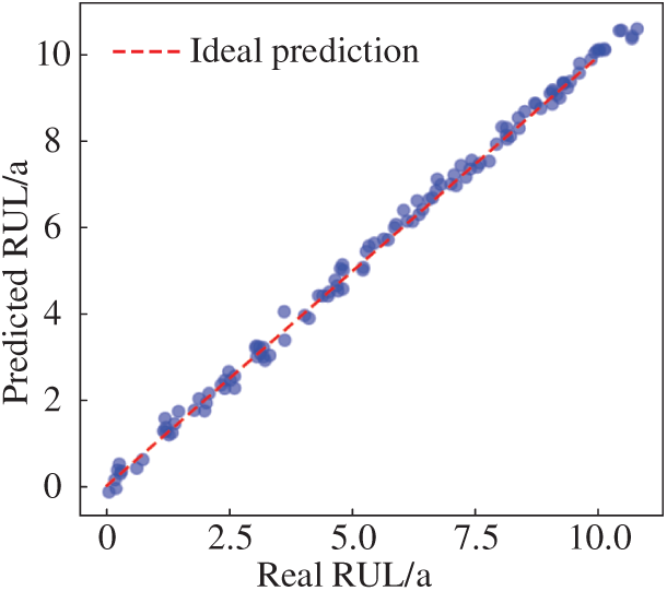
Figure 9: The RUL prediction results of the Transformer model

From Fig. 9, it is evident that the scatter describing the relationship between the predicted and actual RUL values lies almost on the line y=x, demonstrating that the Transformer-driven RUL estimation scheme can produce more precise system-level remaining-life forecasts. Considering that there is a large amount of prediction data, Fig. 10 only shows the RUL probability distribution of some samples within the 95% confidence interval.

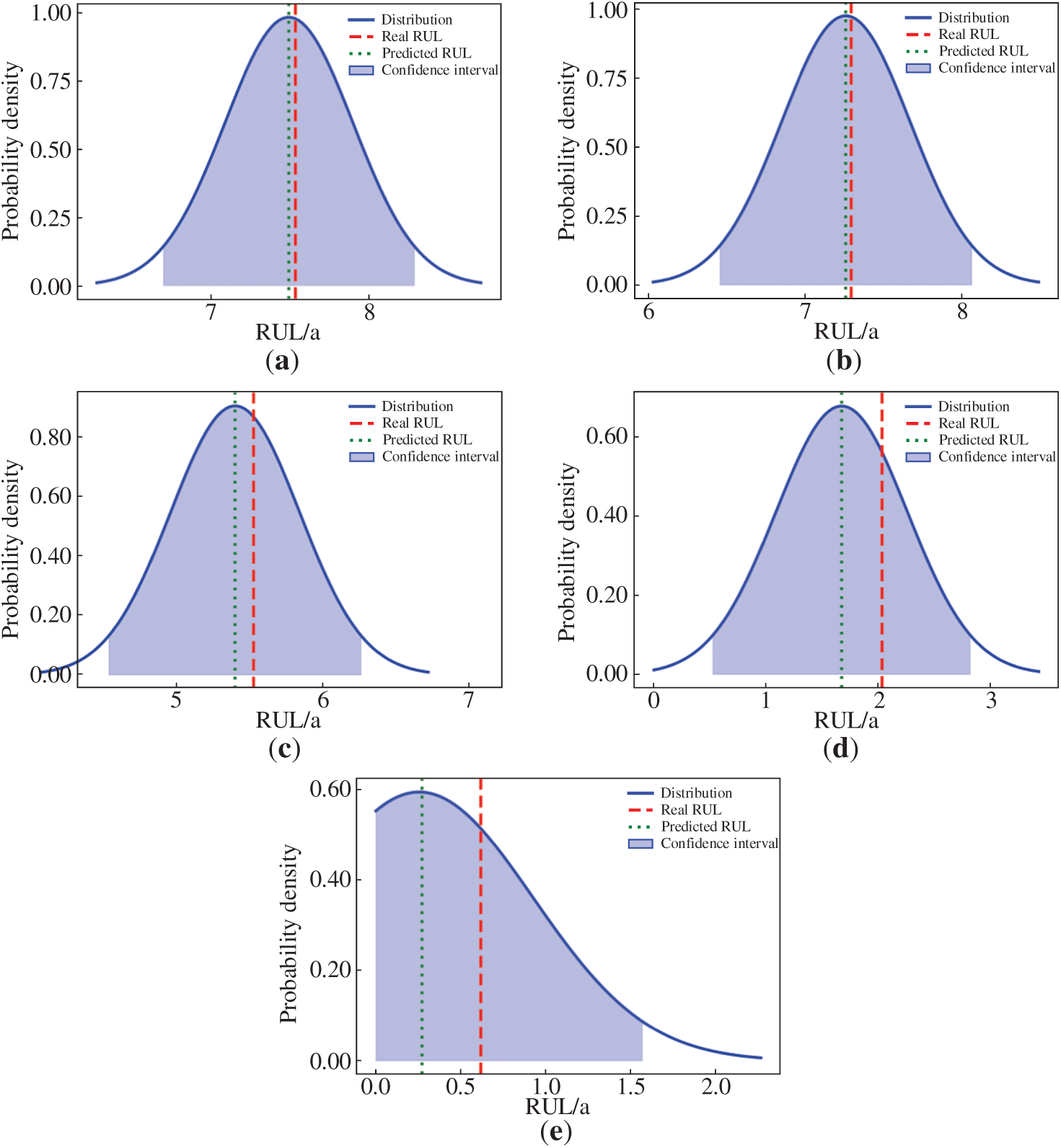
Figure 10: The probability distribution of RUL for some samples. (a) RUL distribution of Sample 1 (b) RUL distribution of Sample 2 (c) RUL distribution of Sample 3 (d) RUL distribution of Sample 4 (e) RUL distribution of Sample 5

As can be seen from Fig. 10, in the samples randomly selected at different stages, the RUL prediction model proposed in this study was able to predict the remaining useful life of each sample, verifying the effectiveness of the model. Then, the RUL prediction results of all samples were statistically analyzed and averaged to obtain the correlation information between the degradation rate of the system’s output power and the average RUL, as shown in Fig. 11.

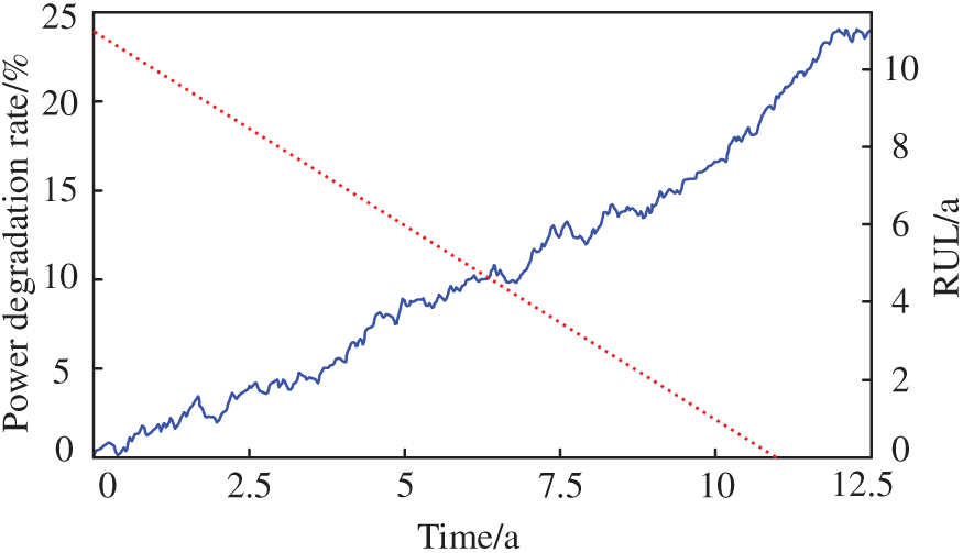
Figure 11: Correlation information between output power and RUL

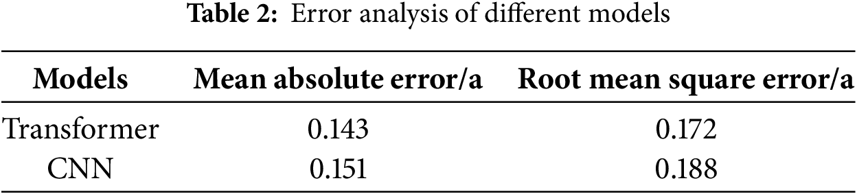
Finally, in order to verify the effectiveness of the method proposed in this paper, the prediction results of the Transformer model and the CNN model were compared. The prediction results of the CNN model are shown in Fig. 12.

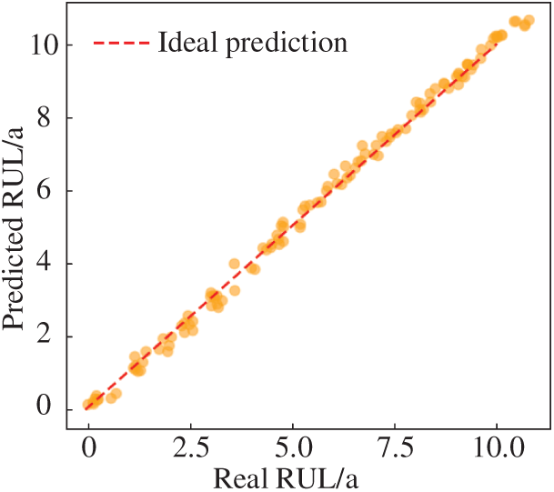
Figure 12: The RUL prediction results of the CNN model

As can be seen from Fig. 12, although the CNN model can also predict the remaining useful life of the system with relatively high accuracy, the number of points deviating from the ideal prediction curve is greater than that of the Transformer model. Finally, Table 2 summarizes the error analysis of RUL prediction using the Transformer model and the CNN model.

4.2 Predictive Maintenance Strategy for PV Power System Based on RUL Information

4.2.1 Relevant Maintenance Information

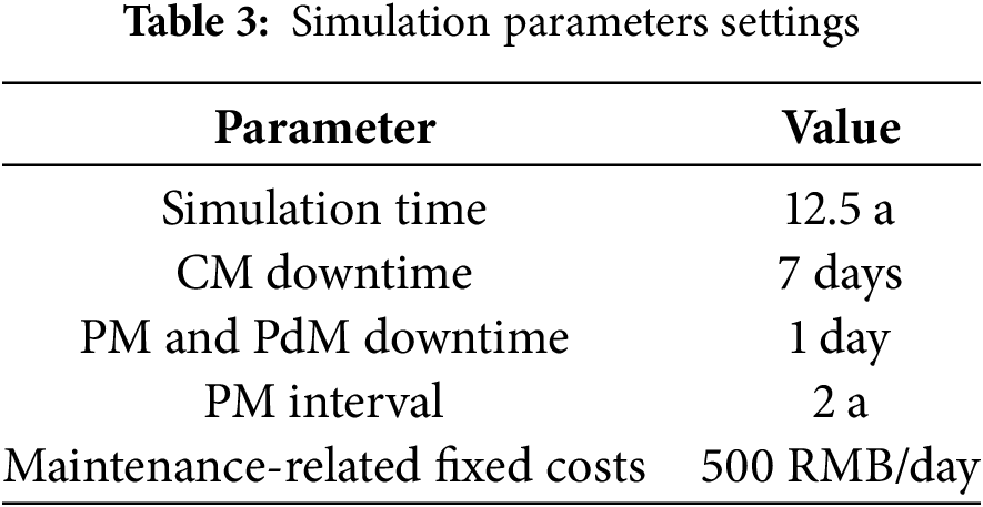
The simulation parameters for this study are shown in Table 3. Among them, the expected lifespan of the system when no maintenance decisions were involved was 10.9 years.

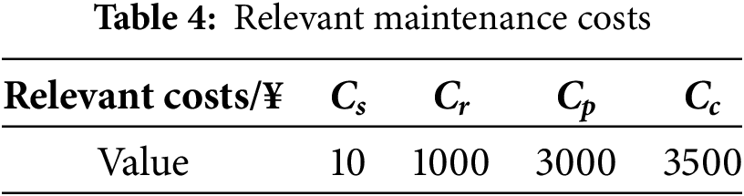
Suppose that the monitoring activities need to be carried out every day, referring to the literature [25], the relevant maintenance cost information is obtained as shown in Table 4, where Cs denotes the cost of unit condition monitoring, Cr denotes the cost of maintenance preparation, Cp denotes the average cost of PM and PdM, and Cc denotes the average cost of CM.

4.2.2 Comparative Analysis of Different Algorithms

This subsection searches for the optimal cost ratio and its corresponding algorithm by comparing and analyzing the convergence of HHO with OHHO and other improved HHO [26,27]. The convergence curves of the algorithms as well as the computational time comparisons are shown in Figs. 13 and 14, respectively.

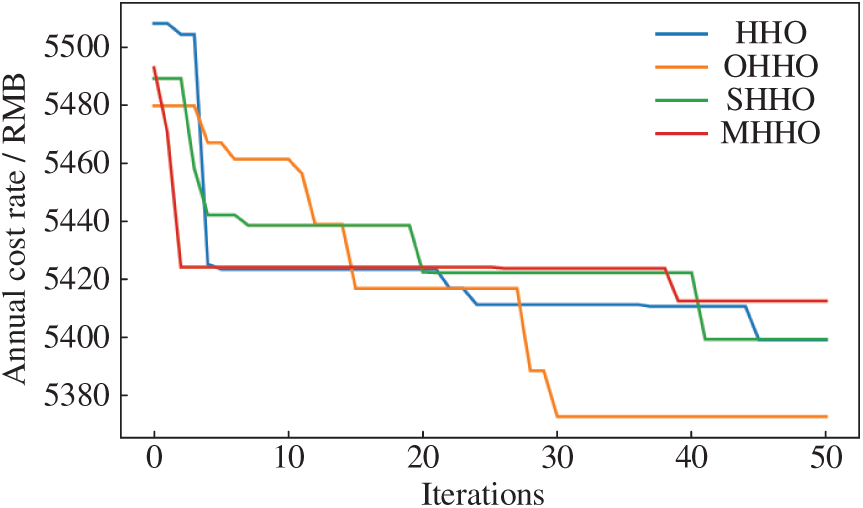
Figure 13: Convergence curves of each HHO

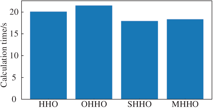
Figure 14: Calculation time for each HHO

Combining Figs. 13 and 14, the performance differences between HHO and each improved form of HHO in maintenance strategy optimization are compared and analyzed. It can be seen that each improved form of HHO can converge to a more optimal solution in fewer iterations, but the optimal solution of OHHO is smaller than the optimal solutions of several other improved forms, showing that OHHO has better convergence performance. And the overall computational time difference among the HHOs is not significant. In the comprehensive analysis, under the objective of minimizing the annual cost rate, OHHO combines good performance with the least computation time, making it ideally suited to the performance demands of a PdM scheme in photovoltaic power systems. The cost analysis of the PdM strategy is given in Fig. 15.

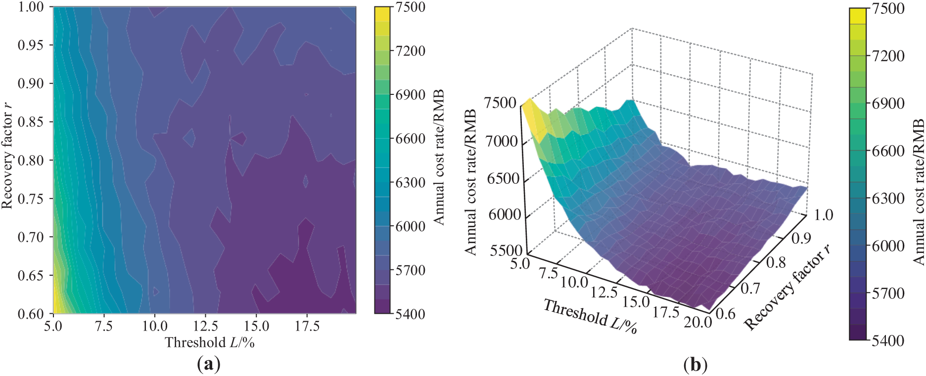
Figure 15: Cost analysis of PdM. (a) Cost plan; (b) Threshold-recovery factor-annual cost rate relationship plot

Considering that in practical engineering applications, the threshold L is difficult to be precisely matched, and the recovery degree is also difficult to be precisely determined, in this case, the concept of “maintenance cost economic basin” is introduced. Combined with Fig. 15 and the algorithm optimization results, if the cost rate does not exceed 103% of the optimal cost rate, then this cost rate is within the “maintenance cost economic basin”, which means that the threshold range is 15%–20%, the recovery factor range is 0.60–0.72, and the annual cost rate meets the above requirements for all combinations of L and r. Based on this, when the system RUL is only about 1.9 a left, corresponding levels of maintenance can be considered. Maintenance actions located within the “maintenance cost economic basin” are called “actionable actions”, and such actions can approximately achieve the optimal annual cost rate. Therefore, the corresponding maintenance actions can be adjusted according to the actual engineering situation, thereby effectively increasing the RUL of the system.

4.2.3 Comparative Analysis of Maintenance Strategies

In order to demonstrate that the PdM strategy of the photovoltaic power generation system has certain advantages over other maintenance strategies, in this study, the cost rates under the CM, PM, and PdM strategies were compared and analyzed through simulation. The results are shown in Table 5.

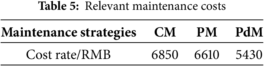
As shown in Table 5, the PdM strategy performs better in minimizing the downtime cost. Compared with the CM and PM strategies, its annual cost rate can be reduced by approximately 20.7% and 17.9%, respectively. However, since the simulation only considered the ideal situation and assumed that the downtime after a failure was relatively short, the cost rates of the three strategies during the maintenance period were quite similar. But in actual engineering, due to many uncontrollable factors such as adverse weather conditions, spare parts issues, and the efficiency of manual maintenance, longer downtime due to failures may occur, which in turn leads to changes in the cost rates. At the same time, due to unplanned downtime, additional costs such as grid penalties and secondary damage to equipment may also be incurred. After comprehensive consideration, the PdM strategy based on RUL information can minimize the cost losses.

4.2.4 Sensitivity Analysis

In order to determine the degree of influence of maintenance threshold, recovery factor and monitoring cost per unit time on the cost rate of the PdM strategy for PV power systems, this paper conducts a sensitivity analysis of the cost parameters of the maintenance model, and analyzes the influence of this parameter on the cost rate by fixing the rest of the parameters and varying a certain parameter. The results of the analysis are shown in Fig. 16.

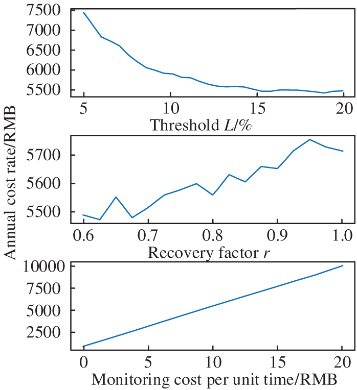
Figure 16: Sensitivity analysis

As shown in Fig. 16, for the PdM strategy of the photovoltaic power generation system, premature maintenance will lead to an excessively high cost rate; excessive maintenance or insufficient maintenance will also increase the maintenance cost; the impact of the recovery factor on the cost rate needs to be comprehensively evaluated in combination with the maintenance threshold; and as the monitoring cost per unit time increases, the annual cost rate will also increase accordingly.

5  Conclusion

This study proposes a (PdM) strategy for PV power systems that uses RUL information, and it derives the following conclusions from simulation analysis:

(1)   In the stage of RUL prediction, the RUL prediction model based on the Transformer model, by learning the degradation law of the device, can achieve the purpose of predicting the RUL of the device by using the fragment data with high accuracy.

(2)   During the design stage of the equipment maintenance strategy, the proposed PdM strategy, by continuously monitoring the RUL information of the photovoltaic power generation system, incorporating the maintenance recovery factor, and using OHHO to find the lowest annual cost rate, can effectively prevent the occurrence of over-maintenance and under-maintenance events, extend the remaining service life of the photovoltaic power generation system, and increase the photovoltaic power generation revenue.

(3)   Unlike other maintenance strategies, the PdM strategy for PV power generation system based on RUL information does not give a specific downtime moment, but utilizes the threshold and recovery factor information provided by the “maintenance economic basin” to give a maintainable interval, which can be better applied to the actual project.

In this paper, the RUL prediction stage is modeled only based on the Transformer model, which leads to a weak ability to extract local degradation information, and the subsequent consideration will be given to adding relevant modules to improve the accuracy of the model prediction. Meanwhile, the validity of this framework needs to be verified on a wider range of types, scales and under different climatic conditions for photovoltaic systems, this aspect will be explored in the next stage of the research.

Acknowledgement: Not applicable.

Funding Statement: This research was supported by the National Natural Science Foundation of China (No. 51767017), the Key Research and Development Program of Gansu Province (No. 25YFGA032), and the Industry Support and Guidance Project for Higher Education Institutions of Gansu Province (No. 2022CYZC-22).

Author Contributions: The authors confirm contribution to the paper as follows: study conception and design: Wei Chen, Yang Wu; data collection: Yang Wu, Guojing Yuan; analysis and interpretation of results: Tingting Pei, Jie Lin; draft manuscript preparation: Yang Wu, Guojing Yuan. All authors reviewed the results and approved the final version of the manuscript.

Availability of Data and Materials: Data supporting this study are included within the article.

Ethics Approval: Not applicable.

Conflicts of Interest: The authors declare no conflicts of interest to report regarding the present study.

References

1. Rajput P, Singh D, Singh KY, Karthick A, Shah MA, Meena RS, et al. A comprehensive review on reliability and degradation of PV modules based on failure modes and effect analysis. Int J Low Carbon Technol. 2024;19:922–37. doi:10.1093/ijlct/ctad106. [Google Scholar] [CrossRef]

2. Abdulla H, Sleptchenko A, Nayfeh A. Photovoltaic systems operation and maintenance: a review and future directions. Renew Sustain Energy Rev. 2024;195(3):114342. doi:10.1016/j.rser.2024.114342. [Google Scholar] [CrossRef]

3. Marangis D, Tziolis G, Livera A, Makrides G, Kyprianou A, Georghiou GE. Intelligent maintenance approaches for improving photovoltaic system performance and reliability. Sol RRL. 2025;9(16):2500289. doi:10.1002/solr.202500289. [Google Scholar] [CrossRef]

4. Peters L, Madlener R. Economic evaluation of maintenance strategies for ground-mounted solar photovoltaic plants. Appl Energy. 2017;199(7):264–80. doi:10.1016/j.apenergy.2017.04.060. [Google Scholar] [CrossRef]

5. Saltmarsh EA, Mavris DN. Simulating corrective maintenance: aggregating component level maintenance time uncertainty at the system level. Procedia Comput Sci. 2013;16:459–68. doi:10.1016/j.procs.2013.01.048. [Google Scholar] [CrossRef]

6. Chen W, Li M, Pei T, Sun C. Research on opportunity maintenance strategy for PV power generation systems considering random impact. Electr Eng. 2024;106(6):7819–30. doi:10.1007/s00202-024-02470-0. [Google Scholar] [CrossRef]

7. Oviedo EHS, Travé-Massuyès L, Subias A, Pavlov M, Alonso C. Detection and classification of faults aimed at preventive maintenance of PV systems. arXiv:2306.08004. 2023. [Google Scholar]

8. Chen W, Li M, Pei T, Sun C, Lei H. Reliability-based model for incomplete preventive replacement maintenance of photovoltaic power systems. Energy Eng. 2023;121(1):125–44. doi:10.32604/ee.2023.042812. [Google Scholar] [CrossRef]

9. Chen W, Sun C, Pei T, Li M, Lei H. Opportunistic maintenance strategies for PV power systems considering the structural correlation. Electr Eng. 2024;106(4):3947–59. doi:10.1007/s00202-023-02182-x. [Google Scholar] [CrossRef]

10. Zhang C, Zeng Q, Dui H, Chen R, Wang S. Reliability model and maintenance cost optimization of wind-photovoltaic hybrid power systems. Reliab Eng Syst Saf. 2025;255(7):110673. doi:10.1016/j.ress.2024.110673. [Google Scholar] [CrossRef]

11. Ledmaoui Y, El Maghraoui A, El Aroussi M, Saadane R. Review of recent advances in predictive maintenance and cybersecurity for solar plants. Sensors. 2025;25(1):206. doi:10.3390/s25010206. [Google Scholar] [PubMed] [CrossRef]

12. Chang Z, Han T. Prognostics and health management of photovoltaic systems based on deep learning: a state-of-the-art review and future perspectives. Renew Sustain Energy Rev. 2024;205(4):114861. doi:10.1016/j.rser.2024.114861. [Google Scholar] [CrossRef]

13. Hua C, Kuang L, Pi D. Maintenance and operation optimization algorithm of PV plants under multiconstraint conditions. Complexity. 2020;2020(1):7975952. doi:10.1155/2020/7975952. [Google Scholar] [CrossRef]

14. Liu Q, Hu Q, Zhou J, Yu D, Mo H. Remaining useful life prediction of PV systems under dynamic environmental conditions. IEEE J Photovolt. 2023;13(4):590–602. doi:10.1109/JPHOTOV.2023.3272071. [Google Scholar] [CrossRef]

15. Lin J, Shen H, Pei T, Wu Y. A two-stage Wiener degradation model-based approach for visual maintenance of photovoltaic modules. Energy Eng. 2025;122(6):2449–63. doi:10.32604/ee.2025.065163. [Google Scholar] [CrossRef]

16. Marangis D, Livera A, Tziolis G, Makrides G, Kyprianou A, Georghiou GE. Trend-based predictive maintenance and fault detection analytics for photovoltaic power plants. Sol RRL. 2024;8(24):2400473. doi:10.1002/solr.202400473. [Google Scholar] [CrossRef]

17. Hamza A, Ali Z, Dudley S, Saleem K, Uneeb M, Christofides N. A multi-stage review framework for AI-driven predictive maintenance and fault diagnosis in photovoltaic systems. Appl Energy. 2025;393(2):126108. doi:10.1016/j.apenergy.2025.126108. [Google Scholar] [CrossRef]

18. Wang J, Xu D, Li Y, Shahidehpour M, Yang T. Transformer-based probabilistic demand forecasting with adaptive online learning. Electr Power Syst Res. 2025;240(2):111255. doi:10.1016/j.epsr.2024.111255. [Google Scholar] [CrossRef]

19. Jin H, Ru R, Cai L, Meng J, Wang B, Peng J, et al. A synthetic data generation method and evolutionary transformer model for degradation trajectory prediction in lithium-ion batteries. Appl Energy. 2025;377(14):124629. doi:10.1016/j.apenergy.2024.124629. [Google Scholar] [CrossRef]

20. Caballé NC, Castro IT. Assessment of the maintenance cost and analysis of availability measures in a finite life cycle for a system subject to competing failures. OR Spectr. 2019;41(1):255–90. doi:10.1007/s00291-018-0521-7. [Google Scholar] [CrossRef]

21. Brown M, Cohen JE. Markov’s inequality: sharpness, renewal theory, finite samples, reliability theory. Commun Stat Theory Meth. 2023;52(11):3652–60. doi:10.1080/03610926.2021.1977960. [Google Scholar] [CrossRef]

22. Heidari AA, Mirjalili S, Faris H, Aljarah I, Mafarja M, Chen H. Harris Hawks optimization: algorithm and applications. Future Gener Comput Syst. 2019;97:849–72. doi:10.1016/j.future.2019.02.028. [Google Scholar] [CrossRef]

23. Tian FL. Research and application of microgrid optimal scheduling based on multi-strategy harris eagle algorithm [master’s thesis]. Changsha, China: Central South University; 2023. (In Chinese). doi: 10.27661/d.cnki.gzhnu.2023.000970. [Google Scholar] [CrossRef]

24. Zhao Y, Liu H. Opposition-based learning Harris Hawks optimization with steepest convergence for engineering design problems. J Supercomput. 2024;81(1):148. doi:10.1007/s11227-024-06649-x. [Google Scholar] [CrossRef]

25. Lei H. Research on remaining life prediction and maintenance strategies for photovoltaic power generation systems based on wiener process [master’s thesis]. Lanzhou, China: Lanzhou University of Technology; 2023. (In Chinese). doi: 10.27206/d.cnki.ggsgu.2023.000763. [Google Scholar] [CrossRef]

26. Alsokhiry F. Leveraging Harris Hawks optimization for enhanced multi-objective optimal power flow in complex power systems. Energies. 2025;18(1):18. doi:10.3390/en18010018. [Google Scholar] [CrossRef]

27. Su Y, Dai Y, Liu Y. A hybrid parallel Harris Hawks optimization algorithm for reusable launch vehicle reentry trajectory optimization with no-fly zones. Soft Comput. 2021;25(23):14597–617. doi:10.1007/s00500-021-06039-y. [Google Scholar] [CrossRef]