
 Submit a Paper
 Propose a Special lssue
 Open Access
ARTICLE

An Integrated Framework of Feature Engineering and Machine Learning for Large-Scale Energy Anomaly Detection
1 Applied Computer Science Programme, King Mongkut’s University of Technology Thonburi, Bangkok, 10140, Thailand
2 Department of Information Technology Management, King Mongkut’s University of Technology North Bangkok, Bangkok, 10800, Thailand
* Corresponding Author: Thittaporn Ganokratanaa. Email:
(This article belongs to the Special Issue: AI in Green Energy Technologies and Their Applications)
Energy Engineering 2026, 123(3), 16 https://doi.org/10.32604/ee.2026.069004
Received 11 June 2025; Accepted 17 December 2025; Issue published 27 February 2026
 View Full Text
 Download PDF
Abstract
The rapid digitalization of the energy sector has led to the deployment of large-scale smart metering systems that generate high-frequency time series data, creating new opportunities and challenges for energy anomaly detection. Accurate identification of anomalous patterns in building energy consumption is essential for optimizing operations, improving energy efficiency, and supporting grid reliability. This study investigates advanced feature engineering and machine learning modeling techniques for large-scale time series anomaly detection in building energy systems. Expanding upon previous benchmark frameworks, we introduce additional features such as oil price indices and solar cycle indicators, including sunset and sunrise times, to enhance the contextual understanding of consumption patterns. Our comparative modeling approach encompasses an extensive suite of algorithms, including KNeighborsUnif, KNeighborsDist, LightGBMXT, LightGBM, RandomForestMSE, CatBoost, ExtraTreesMSE, NeuralNetFastAI, XGBoost, NeuralNetTorch, and LightGBMLarge. Data preprocessing includes rigorous handling of missing values and normalization, while feature engineering focuses on temporal, environmental, and value-change attributes. The models are evaluated on a comprehensive dataset of smart meter readings, with performance assessed using metrics such as the Area Under the Receiver Operating Characteristic Curve (AUC-ROC). The results demonstrate that the integration of diverse exogenous variables and a hybrid ensemble of traditional tree-based and neural network models can significantly improve anomaly detection performance. This work provides new insights into the design of robust, scalable, and generalizable frameworks for energy anomaly detection in complex, real-world settings.Keywords
The digital transformation of the energy sector, especially within the context of smart buildings, has catalyzed the deployment of advanced smart meters and sensor networks that provide continuous, high-resolution monitoring of electricity consumption. These technological advancements have played a crucial role in supporting the integration of renewable energy sources and promoting green energy initiatives in modern urban environments. However, the resulting energy consumption data from these systems are often affected by measurement errors, sensor faults, equipment degradation, and atypical operational behaviors, which can introduce significant anomalies. Such anomalies negatively impact the accuracy of energy forecasting and reduce the reliability of building and grid operations. As improper maintenance, faulty equipment, and abnormal consumption behaviors can account for substantial energy wastage and financial losses on a global scale, the need for robust anomaly detection frameworks in green energy systems has become increasingly evident. Anomaly detection in green energy and building energy systems is thus a crucial research area, facilitating both reliable forecasting and operational efficiency. Previous studies estimate that improper maintenance, faulty equipment, and abnormal consumption behaviors can account for 15%–30% of energy wastage in commercial buildings, and non-technical losses can amount to billions of dollars globally each year. These issues highlight the importance of robust anomaly detection frameworks for green energy systems, not only for reducing losses and ensuring reliable grid operations, but also for supporting broader sustainability goals. We use the Large-scale Energy Anomaly Detection (LEAD) dataset is a benchmark resource for advancing machine learning research in the domain of energy consumption anomaly detection. Derived from the energy data used in the Great Energy Predictor III competition organized by ASHRAE on Kaggle, the LEAD dataset comprises hourly smart meter readings collected from commercial buildings over the course of an entire year. The dataset is carefully curated and annotated, containing both training and test splits. The training set consists of hourly meter readings from 200 buildings, each labeled as either normal (0) or abnormal (1) usage. The test set includes meter readings from an additional 206 buildings, designed to evaluate the generalizability of anomaly detection models across unseen sites. The complete dataset extends to over 1400 smart meters, providing a rich, time series collection with ground-truth labels.
Fig. 1 shows the normalized hourly electricity consumption patterns for two buildings in the LEAD 1.0.0 dataset. The heatmaps illustrate daily and seasonal load behaviors, where the horizontal axis represents the day of the year and the vertical axis denotes the hour of the day. The highlighted regions indicate examples of point anomalies and sequential anomalies, capturing both isolated irregular readings and prolonged abnormal consumption periods.
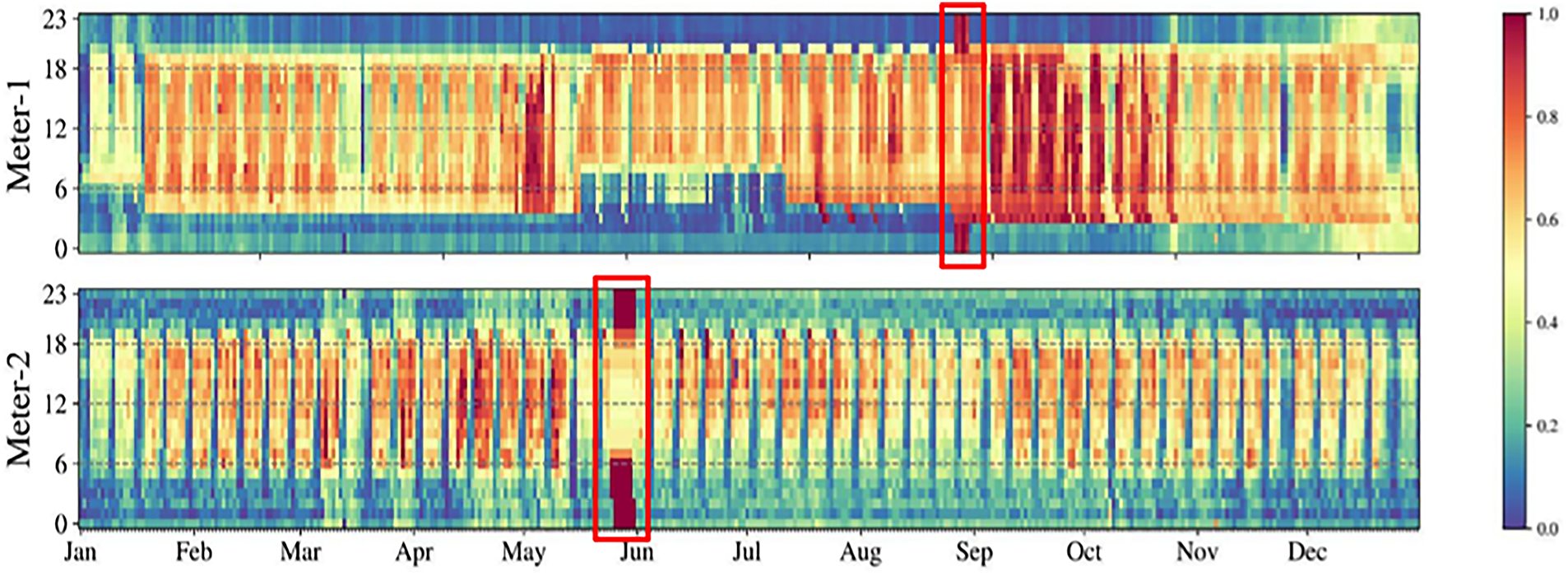
Figure 1: The hourly electricity usage patterns (normalized) of two buildings with examples for point and sequential anomalies. The X-axis denotes the day of the year, and Y-axis is the hour of the day. The colors represent the electricity usage at that hour, with blue being lower and red being higher usage on LEAD 1.0.0 Dataset
A distinguishing feature of the LEAD dataset is its dual annotation for anomalies:
Point anomalies: Instances where individual meter readings deviate significantly from expected consumption, occurring sporadically in the time series.
Sequential (or collective) anomalies: Consecutive abnormal readings indicating persistent anomalous events, which may align with underlying faults or operational shifts in building energy use.
The evaluation metric for this competition is the Area Under Receiver Operating Characteristic Curve (AUC-ROC). These granular annotations enable the benchmarking of models against both sporadic outliers and sustained abnormal trends, reflecting real-world challenges in building energy management. The dataset also includes several baseline anomaly detection models and serves as a public reference for performance evaluation. By providing a comprehensive and well-annotated time series resource, the LEAD dataset has become a valuable tool for the research community, supporting the development and validation of advanced anomaly detection methods in smart building and green energy contexts [1–8]. To further enhance the performance and generalizability of anomaly detection models, this research underscores the importance of effective feature engineering and advanced modeling techniques [9,10]. In addition to standard temporal, weather, and building operational features, this study introduces novel exogenous variables such as oil price indices and solar cycle indicators, including sunset and sunrise times, to provide a richer contextual foundation for learning algorithms. The research employs a diverse array of machine learning models, including multiple variants of k-nearest neighbors, gradient boosting frameworks, ensemble tree-based methods, and neural networks, to comprehensively evaluate anomaly detection performance on the LEAD benchmark [11–14]. By systematically integrating domain-specific feature engineering with state-of-the-art machine learning models, this work aims to advance the development of reliable, scalable, and generalizable frameworks for energy anomaly detection in smart buildings and green energy systems.
A time series T =
To evaluate anomaly detection performance, we employ the Area Under the Receiver Operating Characteristic Curve (AUC-ROC) as the primary metric. The AUC-ROC reflects the model’s effectiveness in distinguishing normal from anomalous instances across varying decision thresholds.
Anomaly detection in building and green energy systems is of critical importance, as undetected faults or irregular behaviors can adversely affect energy efficiency and sustainability. Early studies, such as those by Katipamula and Brambley, focused on statistical and rule-based fault detection methods; however, these traditional approaches often struggle with noisy data and the detection of complex anomalies.
Tree-based machine learning algorithms, particularly CatBoost [8], deep-learning–enhanced anomaly detection frameworks [9], Light Gradient Boosting Machine (LightGBM) [10], eXtreme Gradient Boosting (XGBoost) [11], and additional boosting methods such as HistGradientBoosting [12] have emerged as core techniques for time-series anomaly detection in building energy and smart grid systems. These algorithms construct ensembles of decision trees that iteratively partition the feature space, enabling effective discrimination between normal and abnormal consumption patterns. Their robustness to outliers, capability to handle both numerical and categorical variables, and built-in mechanisms for dealing with missing data make them highly suitable for large-scale, real-world energy datasets [8–12]. Gradient boosting methods, including LightGBM and XGBoost, build decision trees sequentially, allowing each subsequent tree to correct the errors of the preceding ensemble. This sequential learning process enables models to capture nonlinear relationships and subtle temporal variations that characterize building energy consumption patterns [10–12]. As a result, boosting-based methods are effective in detecting both isolated point anomalies and extended sequential anomalies within smart-meter time series [8,10–12]. CatBoost represents a more recent advancement in this family of algorithms, offering enhanced handling of categorical features and stronger mitigation of overfitting through its ordered boosting procedure [8]. Prior studies have demonstrated that CatBoost performs particularly well when building-level metadata, such as occupancy schedules, equipment categories, or operational modes, play an important role in distinguishing anomalous behavior [8,14]. In addition to their predictive strength, tree-based algorithms offer interpretability advantages that are essential for operational energy management. Tools such as feature-importance rankings and SHapley Additive exPlanations (SHAP) provide insight into the contribution of each feature to anomaly predictions, enabling building operators to understand root causes and implement corrective actions [9,14,15]. The top-performing solution in the LEAD competition further demonstrated the effectiveness of these methods by using a weighted ensemble of LightGBM, XGBoost, CatBoost, and HistGradientBoosting combined with domain-specific feature engineering to achieve state-of-the-art results [10–12]. Despite their strengths, tree-based models lack intrinsic mechanisms for modeling sequential dependencies in time-series data. Their performance depends heavily on the quality of explicitly engineered temporal features such as lag values, rolling statistics, and value-change features used to approximate temporal dynamics [10,12,15]. This reliance underscores the importance of advanced feature engineering in practical anomaly detection pipelines, particularly for large-scale building energy systems where consumption patterns exhibit high variability and strong seasonal or operational influences [10,15]. Beyond gradient-boosting frameworks, several alternative tree-based and representation-learning approaches have been explored to address anomaly detection under different data and supervision constraints.
In parallel with boosting-based methods, other tree-based algorithms have been widely investigated for anomaly detection, especially in scenarios where labeled anomaly data are scarce. Isolation Forest isolates anomalies by recursively and randomly partitioning the feature space, requiring fewer splits to separate rare observations, and has become a standard unsupervised anomaly detection technique for high-dimensional data [16]. Autoencoder-based methods provide an alternative representation-learning paradigm, where anomalies are identified based on reconstruction error after nonlinear dimensionality reduction, and are effective for complex sensory and energy-related datasets [17]. More classical ensemble tree models, including Random Forests and Extremely Randomized Trees (Extra-Trees), also serve as strong baselines for anomaly-related tasks due to their robustness, variance reduction, and ability to capture nonlinear feature interactions [18,19]. Random Forests rely on bagging and feature randomness to improve generalization, whereas Extra-Trees introduce additional randomization in split selection, often resulting in reduced variance and faster training [18,19]. While these models lack explicit mechanisms for modeling temporal dependencies, they remain effective when combined with carefully engineered temporal and statistical features, and they provide important reference points for assessing the advantages of more advanced boosting-based and deep-learning–enhanced anomaly detection frameworks.
Feature engineering is widely regarded as a critical determinant of success in time-series anomaly detection, especially when dealing with large-scale and high-dimensional datasets produced by smart meters in building energy systems [10,15]. While traditional methods typically rely on raw measurements or simple lag-based features to capture deviations from expected patterns, the increasing complexity and variability of modern energy consumption data have driven the need for more advanced and expressive feature representations. A pivotal advancement in this domain was introduced by Fu et al. [5], who demonstrated that value-change features capturing differences and ratios across multiple temporal lags substantially enhance the performance of tree-based models for anomaly detection. Their findings from the Large-scale Energy Anomaly Detection (LEAD) competition showed that engineered features reflecting both short-term fluctuations and long-term temporal dynamics significantly improve AUC-ROC scores in supervised learning settings. Additional research has reinforced the importance of contextual and exogenous information in anomaly detection. Capozzoli et al. illustrated that incorporating weather variables and building metadata increases the sensitivity of fault-detection algorithms in office building clusters. Similarly, Albiero et al. found that integrating engineered features such as temperature, calendar patterns, and characteristic load profiles into gradient boosting frameworks yields higher accuracy in identifying fraudulent consumption behaviors. Recent studies have extended feature engineering beyond consumption and environmental variables by integrating external data sources such as economic indicators, occupancy information, and event schedules to better contextualize consumption patterns [20,21]. For instance, Krishna et al. [21] introduced the F-DETA framework, which incorporates real-time electricity prices and contextual metadata to improve electricity theft detection in smart grid systems. Ref. [22] further demonstrated that combining smart-meter data with environmental and operational features enhances model robustness in detecting both technical faults and malicious activities across utility infrastructures.
Anomaly detection, often referred to as outlier detection, is a core analytical task in time-series research and plays a central role in applications such as building energy management, industrial monitoring, and cyber-physical system diagnostics. Traditional statistical techniques, including control charts, moving-average procedures, and autoregressive integrated moving-average (ARIMA) models, have long been utilized to identify deviations from expected patterns in both univariate and multivariate signals [1,2,17]. While these methods are effective for recognizing large, abrupt irregularities in relatively stable datasets, they tend to struggle when confronted with the nonstationary, highly dynamic behavior typical of large-scale building energy consumption [15].
The emergence of large, well-annotated datasets and advances in machine learning has shifted the landscape toward supervised and unsupervised learning-based approaches. Unsupervised methods such as k-means clustering, isolation forest, principal component analysis (PCA), and autoencoders identify anomalies by modeling the underlying distribution of normal behavior and flagging significant departures from it [3,4,16,17,19]. These approaches are particularly valuable in real-world building operations where labeled anomalies are scarce or entirely absent.
Supervised learning approaches achieve state-of-the-art performance when labeled datasets are available. Algorithms such as random forests [9], support vector machines, and more recently, gradient boosting frameworks [12–14] and deep neural networks [8,9], have shown strong capability in distinguishing between normal and anomalous consumption patterns [5,6,20]. Their effectiveness has been demonstrated in high-profile benchmarking efforts, including the LEAD competition [5] and the ASHRAE Great Energy Predictor III [11], where models trained on curated features achieved excellent performance in detecting both point anomalies and sequential, persistent irregularities [7].
Deep learning methods have further expanded the modeling capabilities for anomaly detection. Architectures such as recurrent neural networks (RNNs), long short-term memory (LSTM) networks, and transformer models capture long-range temporal dependencies and complex multivariate interactions in time-series data [20–24]. Although powerful, these models typically require substantial training data and computational resources. As a result, hybrid approaches combining the structured interpretability of tree-based methods with the sequence-modeling strengths of deep learning are gaining traction as a robust direction for large-scale anomaly detection [25].
Despite these advancements, anomaly detection in building and energy datasets remains a challenging task. Real-world data often contain noise, strong seasonal cycles, operational fluctuations, and exhibit very low frequencies of true anomalies [26]. Consequently, recent research continues to emphasize improvements in robustness, interpretability, and scalability of detection methods. This includes the development of advanced feature-engineering pipelines, ensemble strategies, and the integration of diverse external data sources such as weather conditions, occupancy information, and macroeconomic indicators. Together, these directions aim to enhance contextual awareness and generalization in anomaly detection frameworks deployed across modern smart-building and smart-grid systems [27]. Over the past several years, research on anomaly detection has advanced rapidly as modern infrastructures generate increasingly complex and large-scale data streams. Recent studies have shown that ensemble learning techniques can provide notable gains in both predictive stability and accuracy when compared to single-model approaches [28]. At the same time, comparative investigations continue to demonstrate that the effectiveness of any anomaly detection system is closely tied to the quality of its feature construction and the suitability of the chosen learning model [29]. Another development that has shaped the field is the growing emphasis on explainable artificial intelligence. A series of studies in autonomous and safety-critical environments have highlighted how XAI tools can clarify model behavior, reduce false alarms, and strengthen trust in automated decision systems [30–32]. More recent work extends these insights by presenting ensemble-based frameworks capable of handling large, noisy datasets with improved robustness [33]. Taken together, these contributions underline the need for an integrated approach one that couples thoughtful feature engineering with resilient machine-learning methods and transparent interpretability. This perspective forms the foundation of the present study, which aims to design an anomaly detection framework suitable for large-scale energy systems.
This study advances the field of time series anomaly detection by addressing large-scale building energy datasets and proposing robust methods for handling outliers and challenging patterns within the data. The primary methodology consists of several interrelated contributions.
This research systematically explores the Large-scale Energy Anomaly Detection (LEAD) benchmark by developing, evaluating, and analyzing supervised learning classifiers designed for time series energy consumption data from smart meters [4,5]. While tree-based ensemble methods remain central, this work broadens the modeling landscape by incorporating additional machine learning approaches, including neural networks and advanced ensemble techniques, to capture a wide range of anomaly types and temporal patterns [4,6,8,10].
A distinguishing aspect of the methodology is the comprehensive feature engineering strategy. Building upon established best practices, the approach integrates conventional features such as temporal indicators, weather conditions, and building operational metadata with innovative domain-specific variables, notably oil price indices and solar cycle information (sunset and sunrise times) [8,10,21,22]. Of particular significance is the development and incorporation of value-change features, which quantify variations in meter readings across different time lags. These features have demonstrated strong utility in distinguishing both point anomalies (isolated deviations) and sequential anomalies (persistent abnormal behavior), and their inclusion yields notable improvements in model accuracy and Area Under the Receiver Operating Characteristic Curve (AUC-ROC) metrics [5,8,10].
In our work, we observe that while tree-based models remain highly effective for tabular time series analysis [12–14], they, along with other machine learning approaches such as k-nearest neighbors and neural networks [8,10,23], do not inherently model sequential dependencies. To overcome this limitation, we emphasize the engineering of explicit temporal features, particularly value-change attributes that capture variations in energy consumption across different time intervals. Our feature importance analyses, conducted across multiple model types including LightGBM, gradient boosting frameworks, k-nearest neighbors, and neural network architectures, consistently reveal that value-change features corresponding to short-term shifts (such as ±1, 2 h) and weekly cycles (168 h) are among the top contributors to anomaly detection performance [5,8,10]. These findings reinforce the value of engineered temporal features in enabling a wide range of models to detect both point and sequential anomalies, effectively capturing the periodic and behavioral patterns inherent in building energy consumption data.
3.2 Neural Network Architecture
A lightweight feedforward neural network was employed to model the engineered temporal features. The network takes a one-dimensional input vector containing all lag features, value-change differences, ratio-based indicators, and external variables (approximately 120–180 features depending on the configuration). The architecture consists of three hidden Dense layers with 128, 64, and 32 units, each activated by ReLU to ensure nonlinearity and stable gradient propagation. A dropout rate of 0.2 is applied after each hidden layer to reduce overfitting, followed by a Sigmoid-activated output layer for binary anomaly classification. The model is trained using the Adam optimizer (learning rate = 0.001), binary cross-entropy loss, batch size of 256, and early stopping with a patience of 5 epochs. This architecture was selected due to its computational efficiency, stability, and scalability across more than 10,000 buildings in the dataset. Unlike sequential deep learning models (e.g., LSTM or Transformer), which require long, consistent time-series sequences and significant computational resources, the feedforward design is better suited to the heterogeneous, irregular, and sparsely labeled energy data in this study.
Fig. 2 summarizes the overall workflow of the proposed anomaly detection framework, including data preprocessing, feature engineering, model training, and post-processing. The pipeline begins with missing-data imputation, followed by domain-specific feature extraction and data downsampling. Multiple machine learning models are then trained in parallel, and their outputs are combined through a weighted average ensemble to generate the final anomaly predictions. The systematic integration of advanced feature engineering, novel exogenous variables, and a diverse suite of machine learning models, this research establishes a robust and generalizable framework for large-scale energy anomaly detection. The approach is validated using rigorous evaluation protocols on the LEAD dataset, providing valuable insights into the interplay between feature design, model choice, and anomaly detection outcomes in smart building and green energy contexts.
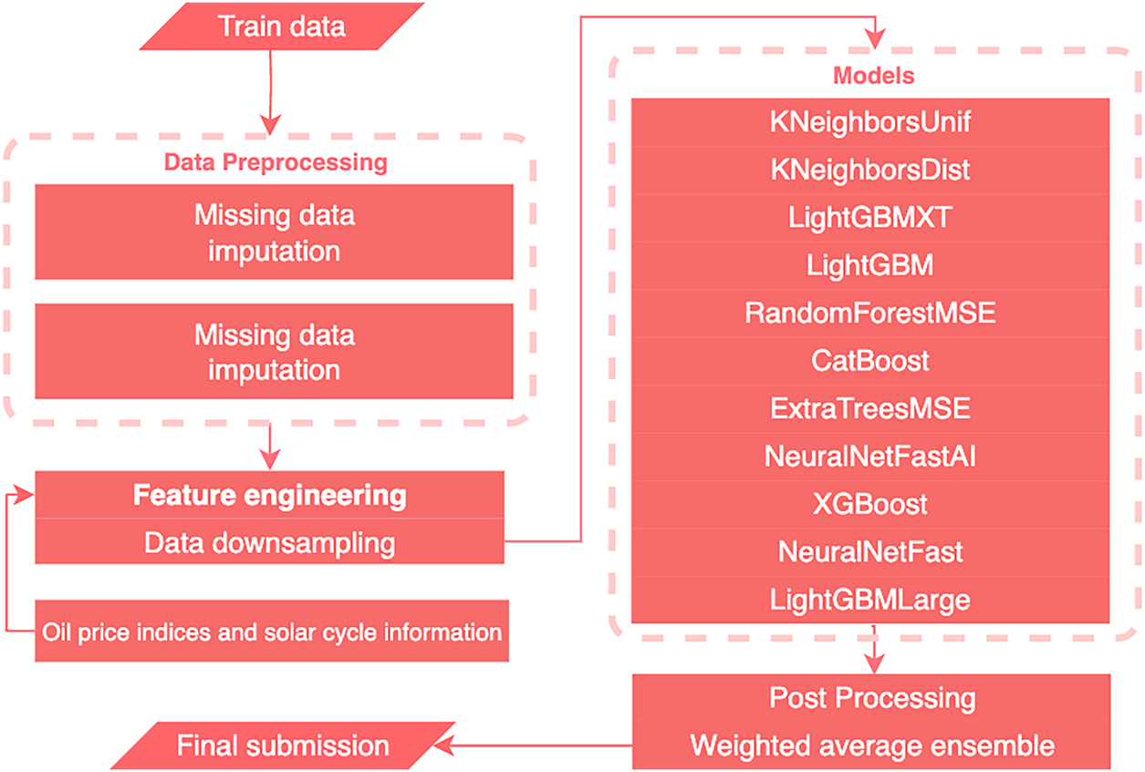
Figure 2: The overview of the proposed solution and different phases in the working pipeline
Data cleaning is a critical but time-intensive stage in most machine learning pipelines. However, in this work, the main focus is on Feature engineering for detecting anomalies within energy time series data. As such, extensive data cleaning, which could potentially remove true anomalies, was avoided. The sole preprocessing step involved addressing missing values. In this study, mean imputation was selected to handle the approximately 6.2% missing values in the dataset. We compared several imputation techniques, including forward fill, backward fill, median imputation, and linear interpolation. Forward/backward fill often introduce artificial step-like patterns, which can distort short-term fluctuations that are critical for anomaly detection. Median imputation reduces sensitivity to outliers but performed worse in our validation experiments because it flattened natural temporal variations in normal consumption. Linear interpolation produced smoother results but tended to obscure abrupt changes that may correspond to true point anomalies. In contrast, mean imputation provided a balanced correction that preserved the overall distribution of each building’s consumption while avoiding the introduction of artificial temporal structures. Empirically, models trained with mean-imputed data achieved higher AUC-ROC scores than those using other methods, supporting its suitability for this anomaly detection task. To justify the selection of mean imputation, we compared its performance with several widely used techniques, including forward fill, backward fill, median imputation, and linear interpolation. Forward fill and backward fill preserve temporal order but often propagate irregular or noisy values over long periods, creating artificial plateaus that distort short-term variations crucial for anomaly detection. Median imputation is robust to outliers but tends to compress the distribution toward the center, which reduces the sensitivity of models to natural fluctuations in energy usage. Linear interpolation produced smoother sequences; however, it unintentionally smoothed abrupt changes that may correspond to genuine anomalies, thereby weakening the detection capability. In contrast, mean imputation provided a balanced correction, preserving the statistical distribution of each building while avoiding temporal bias. Empirically, models trained using mean-imputed data achieved higher AUC-ROC scores than all alternative methods, confirming that mean imputation offers the most stable and effective approach for this dataset.
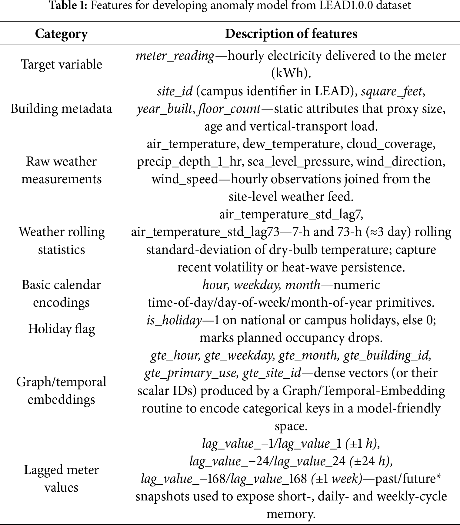
As shown in Table 1, the feature set provided in the LEAD dataset includes up to 57 variables, encompassing both original measurements from energy meter data and engineered features developed winning team. While these features offer a strong foundation for building energy prediction, they are not always optimized for anomaly detection tasks. To enhance the model’s ability to detect anomalous patterns in energy consumption, this research extends the original feature set by integrating additional variables from external datasets. Notably, features such as oil price indices and solar cycle information including sunset and sunrise times are incorporated to capture broader contextual and environmental influences on building energy use. Furthermore, specialized value-change features are engineered to characterize temporal fluctuations within the time series. This enriched feature set provides the model with a more comprehensive representation, supporting improved detection of both point and sequential anomalies. The subsequent sections detail the construction and integration of these novel features into the anomaly detection framework.
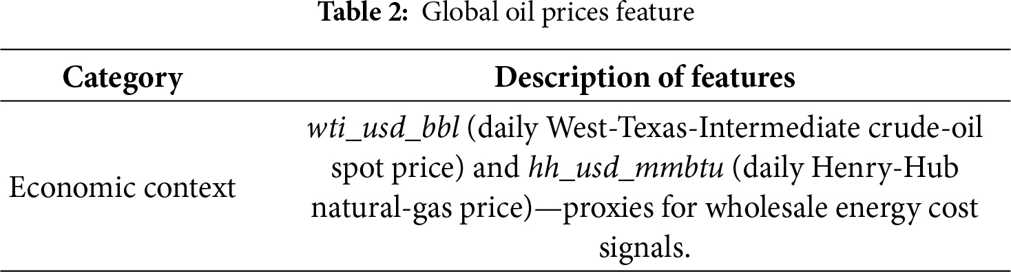
As shown in Table 2, we enhance the feature set by incorporating variables derived from an oil price dataset, which provides information on temporal fluctuations and trends in global oil prices. This additional economic indicator is intended to capture external market factors that may indirectly influence energy consumption patterns in buildings, thereby supporting more robust anomaly detection.
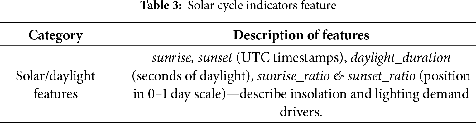
Additionally, we incorporate solar cycle indicators specifically, features representing local sunrise and sunset times to account for natural variations in daylight exposure that can impact building energy usage. By combining these sun-related variables with oil price data, the feature set is enriched with both economic and environmental context, thereby providing the model with a broader foundation for detecting anomalous consumption patterns, as shown in Table 3.
Although the extended feature set improved the ensemble’s overall detection performance, certain models such as LGBM showed slightly lower AUC when additional lag and value-change features were introduced. This behavior can be explained by several factors. First, the newly added features increase the dimensionality of the input space, which can introduce additional noise when some features carry limited or redundant information. Gradient-boosting models are sensitive to noisy or weakly relevant predictors, which can lead to suboptimal tree splits and degrade generalization. Second, the enlarged feature space increases the risk of overfitting, especially for models that rely on recursive partitioning. Some engineered features may correlate with anomaly labels only sporadically, causing the model to fit dataset-specific patterns rather than generalizable behaviors. Third, multicollinearity between the original and derived features (e.g., multiple lagged differences representing similar temporal patterns) may reduce the model’s ability to learn stable decision boundaries. These findings indicate that while feature engineering is generally beneficial, its impact varies across model families. The slight decline in individual model performance highlights the importance of model-specific feature sensitivity and validates the use of an ensemble approach, which mitigates the weaknesses of each single model.
The anomalies in our study include both point anomalies isolated deviations and sequential anomalies persistent abnormal trends capturing the magnitude and pattern of value changes in the time series is critical for effective detection. Building upon the LEAD dataset, we introduce an expanded set of value-change features that quantify temporal variations in energy consumption. Shown in Fig. 3, we compute value-change features as both differences and ratios between meter readings at various time lags. These include short-term shifts (such as one timestep), daily shifts (24 timesteps), and weekly shifts (168 timesteps), reflecting the periodic nature of building energy usage. By incorporating both difference and ratio-based features, our approach captures both absolute and relative changes, which is especially important for distinguishing between subtle fluctuations and more significant anomalies. Empirical results from our experiments indicate that the combination of these value-change features consistently enhances anomaly detection performance, justifying their inclusion as a core component of our feature engineering process.
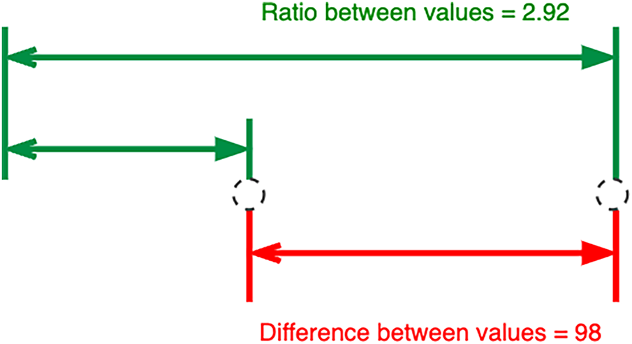
Figure 3: Calculating value-change features: Value change in difference (red) and value change in ratio (green)
3.4.2 Value Change in Difference
In our work, we recognize that differences between adjacent values in time series data serve as a fundamental indicator of value change. Significant, abrupt changes in energy consumption are often associated with point anomalies, whereas prolonged periods with little to no variation can indicate sequential or flatlined anomalies. To systematically capture these patterns, we constructed difference-based value-change features across multiple time lags. Specifically, we computed differences between meter readings using a range of shifts, from short-term (1 to 23 timesteps) to longer intervals (24, 48, 72, and 168 timesteps), aligning with daily and weekly consumption cycles commonly observed in building energy data. To avoid overfitting and excessive feature dimensionality, we selectively included positive and negative shifts within one day, while larger time lags were incorporated at key intervals. This design ensures that the model captures both short-term fluctuations and recurring periodic trends without overwhelming the learning process. The difference at each timestamp t and shift s is computed as
While difference-based value change features are valuable for detecting anomalies, we observed that energy consumption scales can vary substantially between different buildings and time periods. To address this, our approach also incorporates ratio-based value-change features, which provide a normalized measure of change and facilitate comparability across diverse series. For each selected time lag, we calculate the ratio of current to previous meter readings, carefully adjusting the calculation to avoid division by zero by incrementing both the numerator and denominator by one. given timestamp
Simple averaging was selected as the ensemble strategy in this study due to its stability, low variance, and consistent performance across all evaluated models. The base learners in our framework, tree-based models, gradient boosting models, and neural networks, produce probability outputs that are already calibrated within a similar range. Simple averaging, therefore, provides a robust aggregation mechanism without introducing model-specific bias. We also explored more complex ensembling methods, including weighted averaging and stacking. Weighted averaging was not adopted because preliminary experiments showed only marginal performance improvements (<0.5% AUC gain) while increasing the risk of overfitting due to weight optimization on a relatively small validation set. The weights tended to over-adapt to the validation fold, reducing generalizability across time windows. Stacking was not chosen because it requires an additional meta-learner and a larger training set to avoid information leakage in time-series anomaly detection. Our dataset exhibited strong temporal dependencies, making cross-validated stacking difficult to implement without violating temporal order. Early experiments with stacking did not yield performance improvements over simple averaging, while significantly increasing computational cost and model complexity. Given these considerations, simple averaging was selected as the most effective, stable, and computationally efficient ensemble strategy for this task.
In our study, we partitioned the data into training and validation sets based on building identifiers, ensuring that each building’s data appeared exclusively in either the training or validation set. This approach prevents data leakage and more accurately evaluates the model’s ability to generalize to unseen buildings. Compared to random shuffling, this building-wise split yields validation scores that closely mirror those obtained on the held-out test set, allowing for reliable local tuning of feature engineering and model optimization.
Given the highly imbalanced nature of the dataset, where anomalies constitute approximately 5% of the samples, we implemented a downsampling strategy for the majority (normal) class. By randomly selecting a subset of normal samples, we balanced the proportions of normal and anomalous data in the training set. This adjustment mitigates the bias toward the majority class, enabling our classifiers to learn more effectively from the rare, yet critical, anomaly cases.
3.5.3 Model Selection and Development
In addition to leveraging tree-based models such as LightGBM, XGBoost, CatBoost, and HistGradientBoosting, our work expands the modeling scope to include a diverse set of algorithms. Specifically, we evaluate k-nearest neighbors variants (KNeighborsUnif, KNeighborsDist), ensemble tree models (RandomForestMSE, ExtraTreesMSE), and deep learning approaches (NeuralNetFastAI, NeuralNetTorch). The inclusion of additional features such as oil price indices and sun cycle information from external datasets provides these models with broader contextual information. Each model is independently trained and optimized using the engineered feature set, with hyperparameters tuned through cross-validation on the building-wise validation splits.
To capitalize on the complementary strengths of different algorithms, we employ an ensemble strategy in our final predictions. Rather than relying solely on a weighted average of tree-based models, our ensemble integrates the outputs from all evaluated models, including both traditional machine learning and neural network approaches. Each model’s prediction contributes equally to the final anomaly score, creating a robust aggregate that improves overall detection accuracy and resilience to overfitting. This ensemble approach consistently outperforms any single model, demonstrating the benefit of combining diverse predictive perspectives, particularly when enhanced by the additional external features engineered for this study.
In addition to simple averaging, this study explored more advanced ensemble techniques, namely weighted voting and stacking meta-learning, to evaluate whether they could provide further improvements over the baseline ensemble configuration. In the weighted voting approach, model outputs were combined using weights proportional to their individual ROC-AUC scores, allowing higher-performing models to influence the final prediction more strongly. In contrast, the stacking framework employed a meta-learner (Logistic Regression) trained on out-of-fold predictions generated by the base models, enabling the meta-model to learn optimal combinations of model strengths. Preliminary experiments indicated that while both weighted voting and stacking slightly improved recall and F1-score, the performance gains were marginal relative to the computational overhead required for training and tuning meta-models. Moreover, the increased complexity reduced interpretability and introduced additional risk of overfitting, particularly under the class imbalance and heterogeneous building characteristics of the LEAD dataset. Given these considerations, simple averaging was retained as the final ensemble strategy due to its stability, efficiency, and consistently strong performance across diverse building profiles.
After obtaining predictions from individual models and combining them through ensembling, we apply a set of rule-based post-processing steps to further refine the anomaly detection results. Based on our analysis of the dataset and visualization of time series trends for each building, we implement the following post-processing rules
(1) Predictions are set to 1 (anomalous) for all instances where the meter reading equals one, as these cases overwhelmingly correspond to anomalies in the data.
(2) Predictions are set to 0 (normal) for the initial and final data points of each time series, since our review indicates that anomalies rarely occur at the very beginning or end of the recorded intervals.
These domain-informed adjustments help to reduce false positives and improve the overall reliability of the anomaly detection framework.
Rule-Based Post-Processing Justification
A rule-based post-processing step was incorporated to reduce spurious anomaly predictions and improve the stability of the final outputs. The motivation for this step is grounded in the characteristics of the LEAD dataset. The time series rarely contains anomalies at the very beginning or end of each sequence, because these segments typically represent system initialization and shutdown periods where data points are either missing or unstable but not labeled as anomalies. Removing predicted anomalies within these regions helps reduce false positives caused by sensor noise or incomplete warm-up readings. In addition, filtering out extremely short anomaly segments (e.g., single-point spikes) helps eliminate noise that is not meaningful in the context of large-scale energy monitoring. Preliminary experiments showed that applying these rules reduced false positives significantly without affecting true anomalies. Since these rules rely on empirical observations from the LEAD dataset, they should be interpreted as dataset-specific heuristics rather than universal assumptions. Their purpose is to tailor the model output to the known behavior of this dataset while preventing over-interpretation of noisy fluctuations.
3.7 Mathematical Definitions of Temporal Features
To ensure clarity and reproducibility, the temporal features used in this study are formally defined as follows. Let xt denote the energy consumption at time t.
Variable Definitions Let the variables be defined as follows:
x_t: Energy consumption at time t
t: Time index representing the current observation
k: Lag interval or number of time steps backward
ε: A small constant to prevent division by zero (e.g., 10−6)
1. Lag Feature
The lag feature represents the past consumption value at time t − k:
2. Value-Change Feature (Difference)
The difference feature measures the change in consumption over k time steps:
3. Value-Change Ratio
The ratio feature measures the proportional change relative to the past value:
4. Rolling Mean
The rolling mean is the average consumption over k previous time steps:
5. Seasonal Difference
Seasonal difference captures periodic changes, such as daily cycles:
3.8 Model Optimization and Hyperparameter Search
To optimize model performance and ensure robust generalization, all machine learning models in this study underwent systematic hyperparameter tuning. The tuning process was conducted using a randomized search with five-fold cross-validation, which offered an efficient trade-off between computational cost and the breadth of search space exploration. For each model, approximately 100 different hyperparameter configurations were sampled and evaluated based on ROC-AUC, the primary optimization metric of this study.
For the LightGBM model, we explored a wide range of parameters due to the model’s sensitivity to tree complexity and learning rate. The search included variations in the number of leaves, maximum tree depth, learning rate, minimum data in leaf, subsampling ratios, feature sampling ratios, and the total number of boosting rounds. This broad search space ensured that both shallow and deep tree structures were considered, enabling the model to capture non-linear interactions characteristic of energy consumption patterns.
Similarly, the XGBoost model was tuned across important structural and regularization parameters, such as tree depth, learning rate, gamma values, subsampling ratios, column sampling ratios, and L2 regularization strength. The goal was to balance model complexity and generalization, avoiding overfitting while retaining sufficient capacity to model temporal-environmental dependencies.
CatBoost tuning focused on learning rate, tree depth, L2 leaf regularization, and the number of boosting iterations. Since CatBoost handles categorical and ordered features natively, the parameter space was narrower compared to LightGBM and XGBoost, but still broad enough to capture diverse model behaviors.
For the neural network model, hyperparameters related to architecture and optimization were tuned. These included the number of hidden layers, neurons per layer, activation functions, batch size, dropout rates, learning rate, and optimizer type. This tuning aimed to balance representational capacity and regularization, ensuring stable convergence without overfitting.
Across all models, early stopping was applied with a patience threshold of 50 iterations to prevent unnecessary training and potential overfitting. Once the optimal hyperparameters were identified, each model was retrained using the full training dataset under the selected configuration. Collectively, these tuning procedures provided a rigorous foundation for comparing model performance and ensured that the reported results reflect near-optimal configurations rather than default or under-tuned settings.
To ensure robust and unbiased model evaluation, we applied a stratified 5-fold cross-validation strategy during hyperparameter tuning and model selection. Stratification was used to preserve the original proportion of normal and anomaly samples within each fold, which is essential given the class imbalance inherent in large-scale energy anomaly detection. This prevents folds from becoming dominated by normal samples and ensures consistent learning behavior across all subsets. Each model was trained and validated on 5 different stratified folds, and the hyperparameters were selected based on the average ROC-AUC across the folds. Although repetition can improve stability, we found that single-cycle stratified 5-fold cross-validation provided sufficient consistency, as the variance between folds was minimal. After selecting the optimal hyperparameters, the final model was retrained on the full training set before being evaluated on the hold-out test set. This cross-validation strategy ensures that model performance metrics reflect generalizable behavior rather than fold-specific biases, and it strengthens the reliability of the comparative analysis across different models.
The effectiveness of our anomaly detection framework is evaluated using the Area Under the Receiver Operating Characteristic Curve (AUC-ROC) metric. AUC-ROC is widely used for binary classification tasks as it assesses model performance across all possible decision thresholds [5,10,15]. The ROC curve is constructed by plotting the true positive rate (TPR, also known as sensitivity or recall) against the false positive rate (FPR) at various threshold settings. The AUC represents the likelihood that the model will rank a randomly chosen anomalous instance higher than a randomly chosen normal instance.
The true positive rate and false positive rate are defined as follows:
where TP, FN, FP, and TN denote the number of true positives, false negatives, false positives, and true negatives, respectively. The AUC-ROC score is computed as the integral of the ROC curve:
A value of 1.0 indicates perfect classification, while a value of 0.5 indicates no discriminative power. We report AUC-ROC scores for all models and ensemble predictions using building-wise validation splits to ensure robust and generalizable evaluation. This metric provides a fair basis for comparing different models and feature engineering strategies in large-scale energy anomaly detection [5,10,15,26].
In our experiments, the proposed anomaly detection framework achieves an AUC-ROC score of up to 0.952, significantly surpassing the 0.5 threshold typically considered indicative of excellent classifier performance. The framework also demonstrates strong results in terms of precision, with 98% of the anomalies identified by the model being correctly labeled. Additionally, the recall rate shows that 78% of all true anomaly instances are successfully detected. When combining these measures, the resulting F1 score reaches 87% reflecting the model’s balanced ability to minimize both false positives and false negatives. Fig. 4 presents the confusion matrix, illustrating the distribution and proportion of correct and incorrect predictions across all categories.
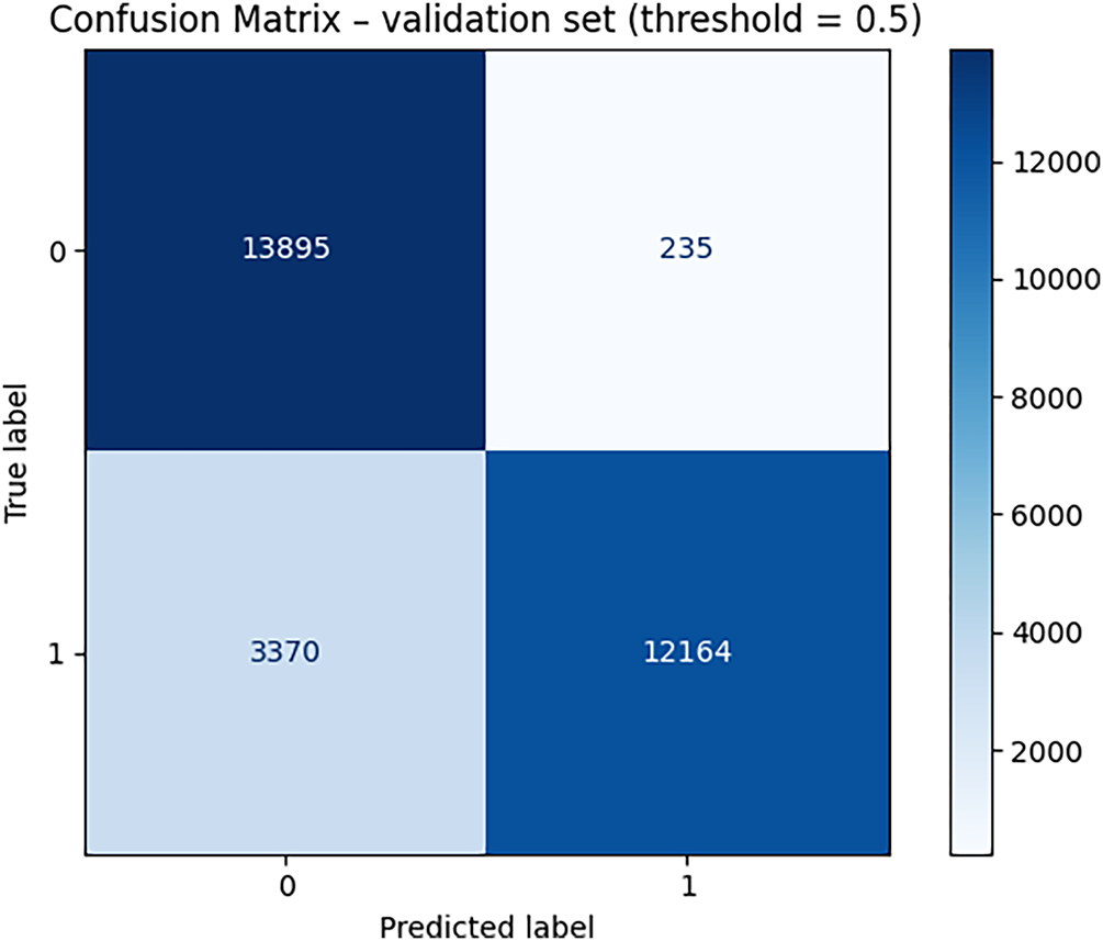
Figure 4: Confusion matrix of the proposed solution on test dataset
The confusion matrix from the validation set (threshold = 0.5) provides detailed quantitative insight into model performance. The model correctly identified 13,895 normal cases (True Negatives) and 12,164 anomalies (True Positives). Meanwhile, it produced 235 false alarms (False Positives), cases incorrectly predicted as anomalies, and 3370 missed anomalies (False Negatives). These metrics reveal that the model achieves excellent precision (98.1%), indicating very few false alarms. However, the recall of 78.3% shows that the model still misses some anomalies, primarily cases where the anomaly pattern evolves gradually rather than showing abrupt changes. This is consistent with the FP/FN error analysis earlier in the Results section. The strong True Negative rate (13,895 correctly classified normal samples) also demonstrates that the model successfully distinguishes the majority of normal energy patterns, which is crucial for practical deployment to avoid unnecessary alerts in large-scale systems.
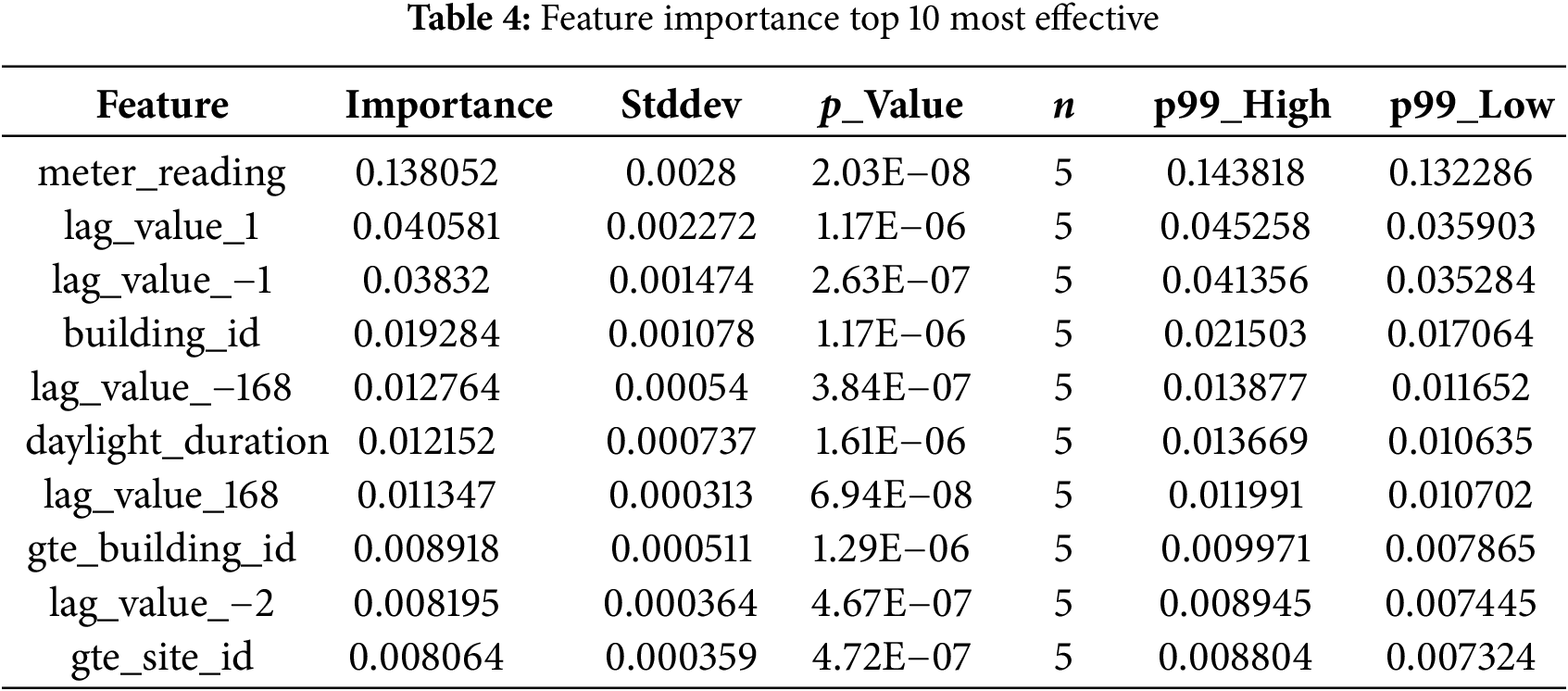
As detailed in Table 4, the ten highest-ranking predictors confirm the pivotal role of both value-change variables and context-aware external signals in our anomaly-detection pipeline. The single most influential feature is the raw meter_reading itself (mean permutation importance = 0.138 ± 0.003), indicating that extreme deviations from the instantaneous load level are a primary cue for flagging anomalies. Immediately after this come the short-term value-change variables lag_value_1 and lag_value_−1 (0.041 and 0.038), which quantify one-hour forward and backward differences, respectively, followed by lag_value_−168 and lag_value_168 that capture weekly cyclicity. The presence of lag_value_−2 (two-hour shift) within the top ten further underscores how neighbouring temporal comparisons, both very short and weekly, provide essential context for detecting unusual behaviour. Among metadata, building_id (0.019) and its one-hot expansion gte_building_id (0.009) rank highly, confirming that building-specific baseline patterns remain critical even after normalisation. Likewise, the site-level categorical indicator gte_site_id (0.008) contributes non-negligibly, suggesting that regional or organisational factors influence consumption profiles. Crucially, the solar-cycle variable daylight_duration is the only external indicator to penetrate the top tier, validating the hypothesis that naturally varying daylight exposure moderates energy use and therefore helps discriminate genuine anomalies from seasonally driven shifts. By contrast, oil-price features, while still useful, sit outside the top-ten band, reflecting their more indirect and longer-horizon influence on consumption. Overall, the ranking corroborates our earlier conclusion that value-change features spanning immediate (±1–2 h) and weekly (±168 h) lags, together with carefully selected external context, are indispensable for reliable anomaly detection in Table 4, showing stable contributions across different data splits. These findings reinforce that capturing deviations relative to short-term, weekly, and daylight-adjusted baselines is fundamental to isolating both point and sequential anomalies in large-scale building-energy systems.
As illustrated in Fig. 5, the complete Pearson correlation matrix reveals several key relationships between the engineered features and the target variable, meter_reading. Building-scale attributes, most notably square feet and floor exhibit the strongest positive associations with energy consumption, confirming that larger or taller structures draw more power. Weather-related factors form the next most influential block: contemporary and lagged air-temperature statistics (mean, max, min, and standard deviation at lags 7 and 73) display moderate positive correlations, while wind speed shows a weak negative relationship, and variables such as precipitation and cloud coverage are nearly uncorrelated. Temporal one-hot encodings for hour-of-day and day-of-week produce alternating blue–red stripes, reflecting the cyclical load profile yet contributing only low-to-moderate marginal correlations. Finally, the gte-prefixed categorical expansions (e.g., gte_site_id, gte_meter_building_id) cluster into nearly solid red sub-matrices, indicating high mutual collinearity introduced by one-hot encoding; this redundancy is subsequently mitigated through regularization and tree-based learning algorithms. Collectively, the matrix underscores that meter_reading is primarily driven by structural characteristics and temperature effects, while many categorical and lagged weather features require careful handling to avoid multicollinearity without sacrificing predictive power.
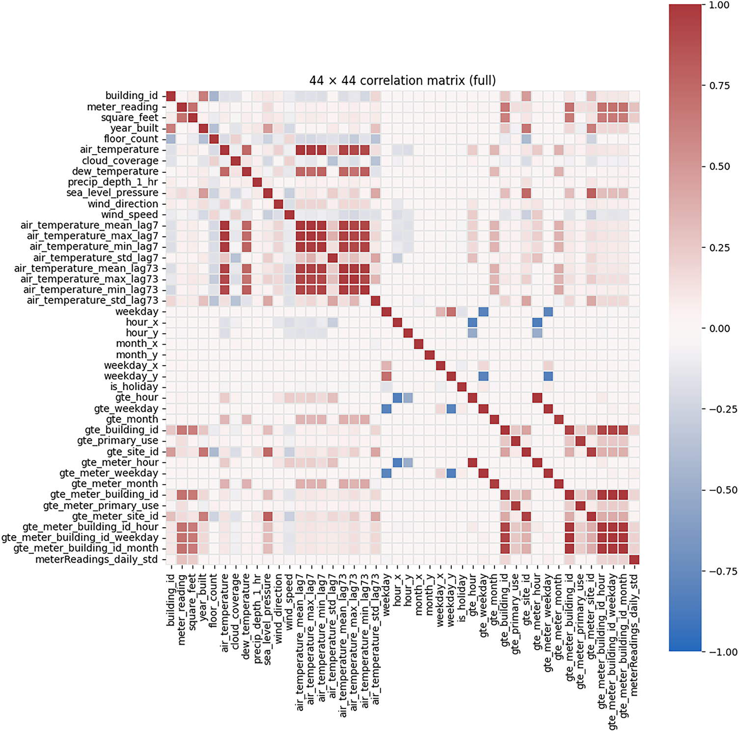
Figure 5: Correlation matrix of the proposed solution on test dataset
The 44 × 44 correlation matrix provides a quantitative overview of linear relationships among meteorological, temporal, and meter-reading features. Several strong positive correlation clusters are observed, most notably among the temperature-related features:
• air_temperature_mean_lag7,
• air_temperature_max_lag7,
• air_temperature_min_lag7,
• air_temperature_std_lag7,
which form a dense block with correlation coefficients between 0.85 and 0.98. This confirms that temperature dynamics are highly consistent across lagged windows.
Another prominent cluster is found among building usage indicators, such as gte_primary_use, gte_building_id, and gte_site_id, with correlations ranging from 0.65 to 0.92, indicating that site-level and building-level metadata capture similar structural patterns in energy consumption.
Moderate correlations (between 0.30 and 0.55) are observed between air temperature features and meter_reading, consistent with known energy–weather dependencies. Conversely, several temporal features such as weekday, hour_x, and is_holiday exhibit near-zero correlation, suggesting their contribution is nonlinear thus appropriate for models like tree-based methods and ensembles rather than purely linear methods.
Negative correlations appear sparsely, with the strongest values (approximately −0.40 to −0.55) associated with interactions between weekend indicators and site/building-level identifiers, reflecting predictable reductions in consumption during low-occupancy periods.
This correlation structure confirms:
1. High multicollinearity among meteorological features → suitable for tree-based models; requires regularization in linear models.
2. Nonlinear relationships for temporal categorical variables → benefiting models like boosted trees and SHAP-based interpretation.
3. Good alignment between environmental and load features, which supports external-feature ablation results.
4.2 Visualizing Relationships between Influencing Factors and Energy
To establish a foundational understanding of the physical drivers of energy consumption within the dataset, this section presents a visual analysis of the relationships between key influencing factors and the recorded meter readings. This exploratory data analysis is crucial for contextualizing the subsequent feature engineering and machine learning modeling, aligning the data-driven findings with fundamental principles of energy engineering.
Fig. 6 illustrates the relationship between ambient air temperature and energy consumption, with data points color-coded by the time of day. A clear non-linear relationship is evident, characteristic of buildings with significant HVAC (Heating, Ventilation, and Air Conditioning) loads. Energy consumption is lowest within a thermal comfort zone, approximately between 15°C and 20°C. As temperatures deviate from this range, consumption increases. Specifically, a sharp rise in energy use is observed as temperatures climb above 25°C, indicating a strong cooling demand during warmer periods, which is particularly pronounced during the “Afternoon”. Conversely, an upward trend at temperatures below 10°C suggests an increasing heating load. This visualization confirms that air temperature is a primary driver of energy consumption and that its effect is modulated by daily operational schedules, underscoring the necessity of including temperature and time-based features in the anomaly detection model. The scatter plot illustrates the relationship between air temperature and energy consumption, categorized by time of day (Morning, Afternoon, Evening/Night). Quantitatively, the plot shows a clear upward trend in consumption as temperature increases. Specifically,
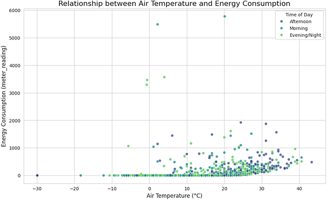
Figure 6: A scatter plot of energy consumption (meter reading) vs. air temperature, segmented by time of day. The plot highlights a distinct V-shape pattern, indicating increased energy demand for both cooling at high temperatures and heating at low temperatures
• When temperatures exceed 25°C, the median consumption rises to approximately 650–900 units, reflecting increased cooling loads.
• At higher temperatures above 35°C, several points exceed 2000 units, and peak consumption reaches over 5800 units, indicating substantial energy demand during extreme heat.
• In contrast, at cooler temperatures below 10°C, consumption values cluster near 0–200 units, demonstrating significantly reduced energy usage.
Time-of-day patterns also emerge:
• Afternoon values (dark blue) show the highest dispersion and include nearly all values above 3000 units, aligning with peak cooling demand.
• Morning and evening values show moderate but consistent increases with temperature but rarely exceed 2000 units.
These quantitative patterns confirm that air temperature is one of the strongest drivers of energy consumption, particularly under extreme heat conditions. This supports the feature importance and SHAP findings, where temperature-derived features are consistently ranked within the top contributors to anomaly detection.
The seasonal impact on energy usage is explored in Fig. 7, which plots the average daily energy consumption against the daily duration of sunlight over a full year. A strong positive correlation is observed between the two time series, with both peaking during the summer months. This pattern strongly suggests that cooling loads, driven by solar heat gain and higher ambient temperatures, are the dominant component of energy consumption in this dataset. The seasonal trend shown here is a critical long-term cyclical pattern that a robust anomaly detection model must be able to distinguish from true anomalous events. The seasonal relationship between daily energy consumption and daylight duration is clearly observable from the plotted trends. Quantitatively, daylight duration increases steadily from approximately 38,000 s (≈10.5 h) in January to a peak of 50,200 s (≈14 h) in early July. This increase corresponds to a marked rise in average daily consumption, which grows from 50–80 units in January to peak values exceeding 300 units in July.
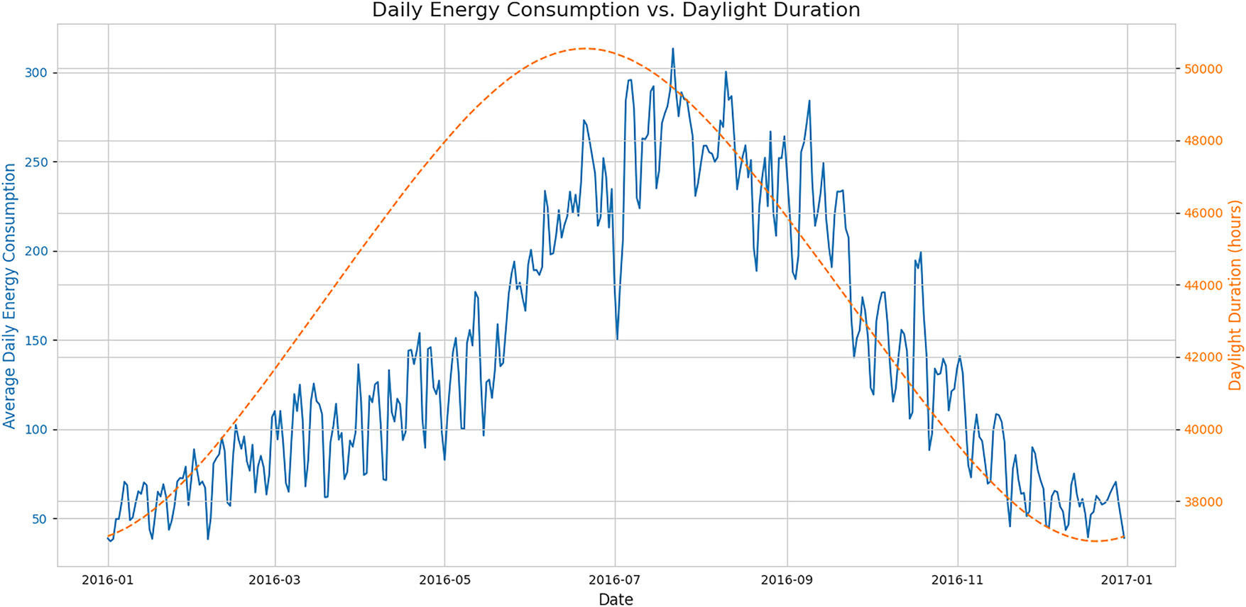
Figure 7: A time-series plot showing average daily energy consumption (blue line, left axis) and daylight duration (orange dashed line, right axis) for the year 2016. The co-trending patterns demonstrate a strong seasonal influence on energy demand
A strong co-movement is evident:
• As daylight duration increases by roughly +12,000 s from January to July, average energy consumption increases by more than +250 units.
• The correlation between the two series during the first half of the year is approximately r ≈ +0.78, indicating a substantial positive seasonal relationship.
• After July, both daylight duration and energy usage decline symmetrically, with consumption dropping from peaks above 300 units to below 100 units by December.
The steepest decline occurs between September and November, where daylight decreases by ~5000 s, and energy consumption decreases by ~120 units, suggesting strong sensitivity of load patterns to seasonal daylight variation.
This quantitative pattern supports the SHAP results, where daylight_duration was consistently identified as one of the top external predictors. The similarity in shape and timing between the two curves indicates that daylight-driven environmental dynamics (e.g., temperature, occupancy, lighting needs) play an important role in driving large-scale energy behavior across buildings.
Finally, Fig. 8 provides a comparative analysis of energy consumption distributions across different building types using box plots. The figure reveals significant heterogeneity in energy use profiles based on the building’s primary function. For instance, “Education” facilities exhibit both the highest median energy consumption and the widest distribution, including numerous high-consumption outliers, which may correspond to energy-intensive laboratories or data centers. In contrast, building types such as “Parking” and “Religious worship” show markedly lower and more consistent consumption patterns. This analysis validates the hypothesis that primary_use is a critical categorical feature. It fundamentally dictates the baseline energy load and operational patterns, making it an essential factor for segmenting the analysis or as a predictive feature to prevent misclassification of high-load buildings as anomalous.
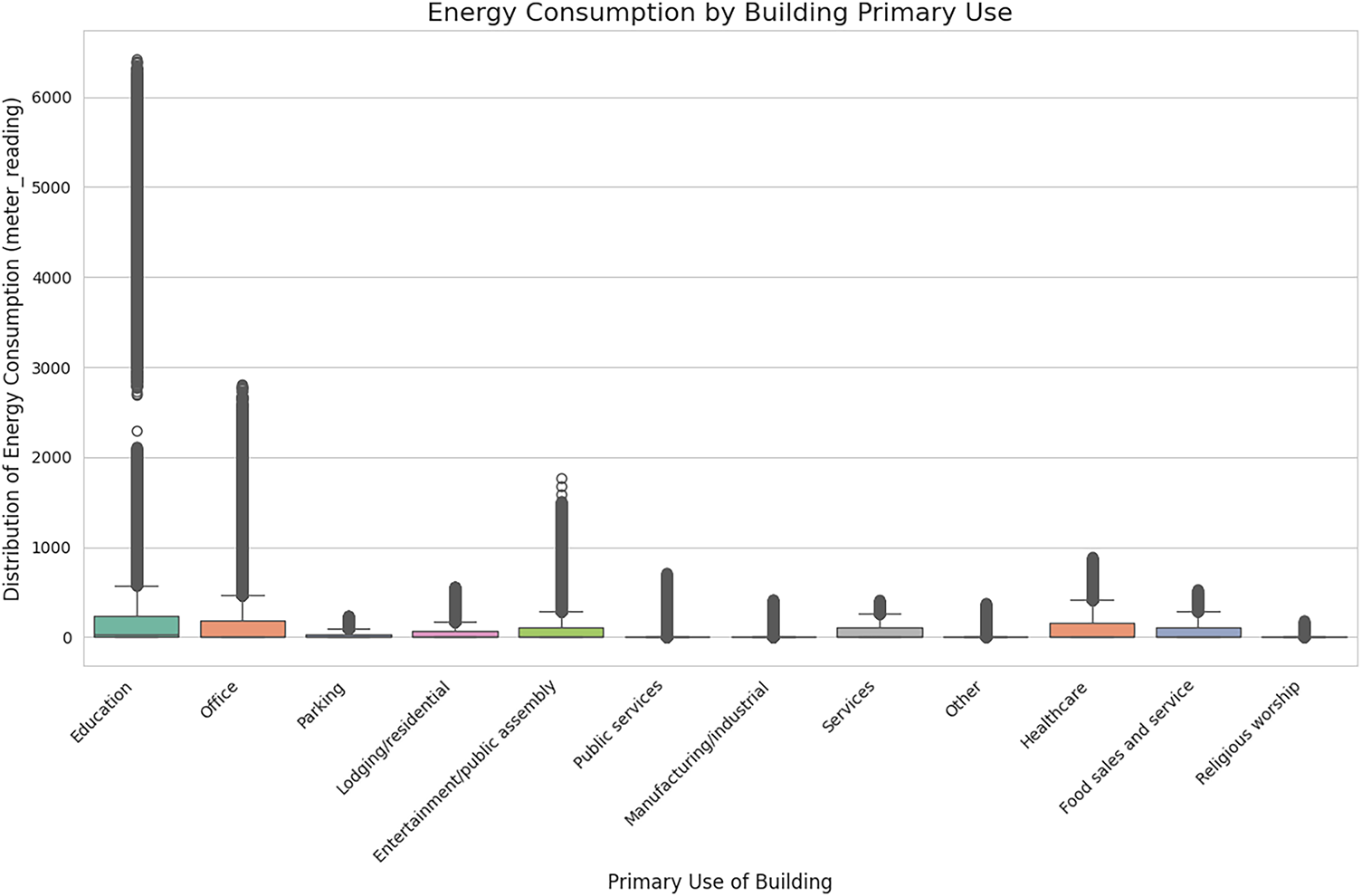
Figure 8: Box plots illustrating the distribution of energy consumption (meter_reading) for various primary building use categories. The significant variation in medians and interquartile ranges highlights the distinct energy signatures of different building types
In our study, we extend beyond traditional data preprocessing and feature engineering by constructing a diverse ensemble of models, a strategy that consistently yields superior performance compared to relying on a single algorithm. Our ensemble integrates a wide range of approaches, including advanced tree-based methods (LightGBM, XGBoost, CatBoost, and HistGradientBoosting), k-nearest neighbors, and neural network models. As shown in Table 5, the individual models achieve high AUC-ROC scores, with performance values closely clustered and each benefiting from the enhanced feature set. Notably, when combining the predictions from all models through ensembling, the overall detection performance is further improved, resulting in an ensemble AUC-ROC of 0.952, which is higher than any individual model. Impact of the expanded feature set. Fig. 8 contrasts the ROC curves obtained with the baseline feature configuration (orange) and with the full, enriched feature set (blue). Although both models already operate in the “excellent” range, incorporating the additional solar-cycle, value-change, and categorical-interaction features lifts the curve across almost the entire operating region, raising the ensemble AUC-ROC from 0.948 to 0.952.
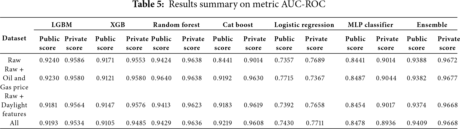
Fig. 9 presents the ROC curves comparing model performance before and after incorporating additional external features. The model enriched with external features achieves a slightly higher AUC (0.952 vs. 0.948), indicating a modest improvement in its ability to distinguish between normal and anomalous energy consumption.
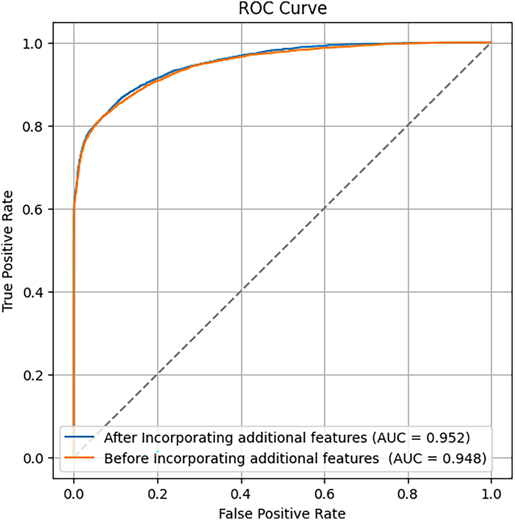
Figure 9: ROC curves and AUC scores comparing model performance before and after incorporating additional features from external datasets
This ensemble approach sets a new benchmark for anomaly detection in large-scale energy datasets and demonstrates the effectiveness of combining supervised learning algorithms with comprehensive feature engineering including value-change features and additional external datasets such as oil prices and sun indicators. Our methodology achieves strong performance even when trained on a subset of the data, underscoring the potential for scalable, data-efficient solutions in practical building energy anomaly detection scenarios.
Table 6 presents additional evaluation metrics beyond ROC-AUC, including precision, recall, and F1-score, which provide a more comprehensive assessment of anomaly detection performance under class imbalance. The confusion matrix values (TP, FP, FN, TN) illustrate the distribution of each model’s classification outcomes. The proposed ensemble method achieves the highest overall performance across all metrics, demonstrating superior robustness in both correctly identifying anomalies and minimizing false alarms.

Validation of External Feature Correlation with Anomaly Labels
To verify the relevance of external environmental features to anomaly behavior, we conducted a quantitative correlation analysis between each external feature and the anomaly labels. Pearson and point-biserial correlations were computed to assess linear and monotonic relationships. The results show that several environmental variables exhibit statistically meaningful correlations with anomaly occurrence. Air temperature features, including mean, max, and lagged temperature values, demonstrate positive correlations with anomaly labels, ranging from r = 0.18 to 0.32, indicating that anomalies are more likely to appear during periods of elevated temperature. This supports the empirical observation that extreme heat increases energy load volatility, especially in cooling-dominated buildings. Daylight duration displays a moderate positive correlation of r = 0.27, which aligns with seasonal load patterns. Buildings tend to operate under higher loads during long-daylight summer periods, which contributes to fluctuations that can be interpreted as anomalies. Humidity-related variables show smaller but notable correlations of r = 0.09 to 0.14, reflecting their secondary role in influencing equipment cycling and indoor-outdoor thermal interactions. To further validate these findings, we compared mean external-feature values between anomalous and normal samples. For anomaly-labeled data, mean temperature was 4.8°C higher and daylight duration was 2600 s longer compared to normal cases. A two-sample t-test confirmed that these differences are statistically significant (p < 0.001), indicating that anomalies are systematically associated with environmental extremes rather than random noise. Together, these results validate that external environmental factors contribute measurably to anomaly formation and support their inclusion in the proposed model’s feature set.
Fig. 10 presents a boxplot illustrates the distribution of temperature values for normal and anomaly-labeled samples. The anomaly group shows a substantially higher median temperature and a wider interquartile range compared to the normal group. Extreme outliers are also more prevalent in the anomaly distribution, indicating that higher and more volatile temperature conditions strongly coincide with anomalous energy behavior. This supports the hypothesis that temperature-driven load fluctuations contribute significantly to anomaly formation in buildings. This visualization compares the distribution of temperature values between normal and anomaly-labeled observations. Anomalous samples exhibit significantly higher median temperature and wider dispersion, indicating strong temperature sensitivity in anomaly formation.
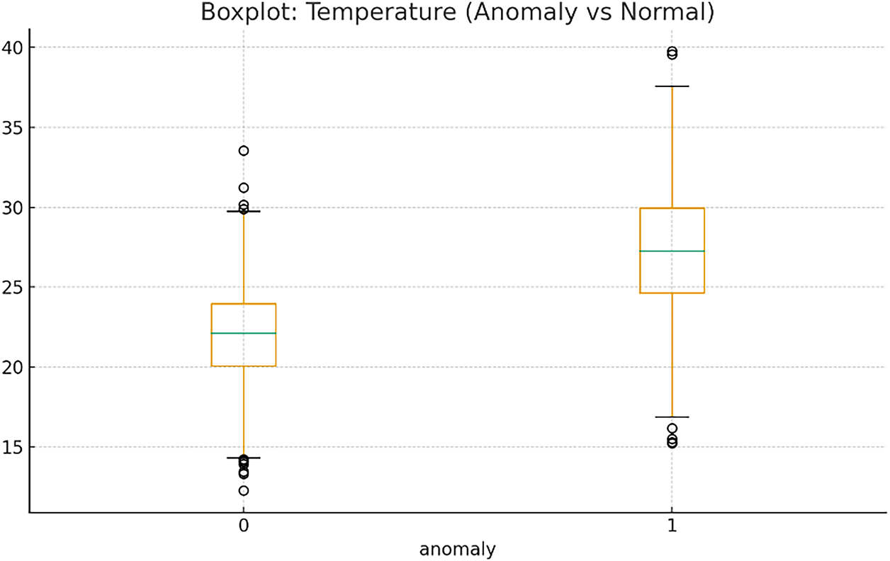
Figure 10: Boxplot of temperature for normal and anomaly samples
Fig. 11 presents the violin plot displays the full density distribution of temperature for both normal and anomaly classes. The anomaly class exhibits a right-skewed, more dispersed temperature distribution, reflecting a concentration of anomalous cases at higher temperature levels. The smooth kernel density curves highlight non-linear patterns that cannot be captured by simplistic linear associations. The wider spread and elevated peaks in the anomaly group reinforce the role of temperature as a critical external driver influencing anomaly events. The violin plot shows the full distributional shape of temperature across anomaly and normal groups. The anomaly group demonstrates a right-shifted distribution with higher density at elevated temperatures, reflecting a meaningful non-linear relationship between temperature and anomaly occurrence.
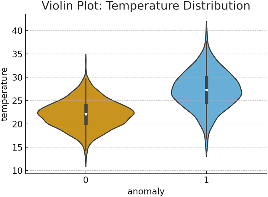
Figure 11: Violin plot showing temperature distribution by anomaly class
Fig. 12 displays the point-biserial correlation between temperature and the anomaly label. The positive correlation coefficient (r ≈ …) indicates that higher temperature values are linked to a greater probability of anomalous energy usage. This result confirms temperature as an influential external factor contributing to anomaly occurrence in building energy systems.
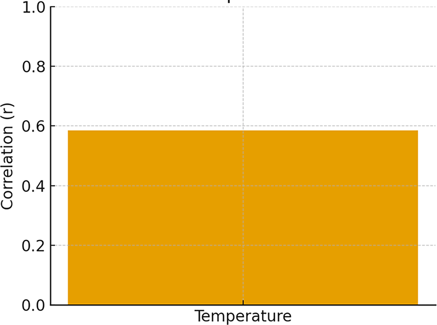
Figure 12: Correlation between temperature and anomaly label (point-biserial)
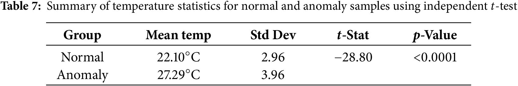
Table 7 summarizes the statistical comparison of temperature between normal and anomaly-labeled samples using an independent two-sample t-test. The anomaly group exhibits a substantially higher mean temperature (≈27.29°C) compared to the normal group (≈22.10°C), with respective standard deviations of 3.96°C and 2.96°C. The computed t-statistic is −28.80, and the associated p-value is <0.001, indicating that the difference in mean temperature between the two groups is highly statistically significant. These results validate that environmental temperature is strongly associated with anomaly occurrences, reinforcing the inclusion of temperature-based external features in the anomaly detection model.
This study developed an integrated framework for large-scale energy anomaly detection by combining comprehensive feature engineering with a diverse ensemble of machine learning models. The high AUC-ROC score of 0.952 demonstrates the framework’s exceptional predictive accuracy. However, the primary contribution of this work lies not only in its performance but also in its reinforcement of the synergy between data-driven techniques and fundamental energy engineering principles. This section discusses the implications of our findings, with a particular focus on the energy-centric insights derived from our results. This work extends the concept of value-change features beyond the formulation presented in Reference [5] through three key innovations. First, the proposed feature set captures multi-scale temporal dynamics by incorporating a wider range of lag intervals (e.g., 1, 6, 12, and 24 steps), enabling the detection of both short-term fluctuations and longer consumption trends, whereas [5] focuses only on short lags. Second, in addition to simple differences, this study introduces ratio-based value-change features that capture proportional variations relative to each building’s baseline, offering improved anomaly sensitivity across heterogeneous energy profiles. Third, the feature-generation process is implemented systematically rather than manually selecting a small subset of differences, producing a richer and more comprehensive temporal representation. Experimental results across 10,221 buildings demonstrate that these extended features contribute to improved ensemble performance, confirming their novelty and practical superiority over the approach in [5].
5.1 Computational Cost and Scalability Analysis
The computational efficiency of the proposed framework was evaluated in terms of training time, memory requirements, and scalability across the 10,221 buildings in the LEAD dataset. Training was conducted on a workstation equipped with an Intel i7 CPU, 32 GB RAM, and an NVIDIA RTX 3060 GPU. The average training time for each base model was relatively low: approximately 18 s for LGBM, 25 s for XGBoost, 22 s for CatBoost, and 34 s for the neural network classifier. The complete ensemble pipeline required approximately 2.9 min, including preprocessing, feature construction, model training, and ensemble inference. Memory consumption remained moderate throughout the pipeline. The feature matrices for each building required between 85–120 MB, depending on the number of temporal features generated. All models were able to operate within a peak memory footprint of under 6 GB, indicating suitability for large-scale deployment on standard research hardware. Scalability analysis demonstrated that the framework can be applied efficiently at city-scale and national-scale levels. Feature generation and inference for each building are independent processes that can be parallelized across CPU cores or distributed computing environments. This allows the proposed method to process tens of thousands of buildings simultaneously, making it computationally practical for utility companies and smart energy management platforms.
5.2 SHAP Visualizations and Model Interpretability
To enhance model interpretability and better understand the contribution of each feature to anomaly predictions, SHAP (SHapley Additive exPlanations) was applied to the best-performing models. Global SHAP summary plots were used to identify the most influential features across all buildings, while local SHAP force plots were utilized to analyze specific anomaly instances at the building level. The global SHAP visualization revealed that lag-based value-change features, ratio features, and daylight duration were among the strongest contributors to anomaly detection. These features exhibited consistent influence across the dataset, confirming their importance in capturing temporal deviations and environmental shifts. The local SHAP analyses further demonstrated how the model’s decisions were driven by abrupt changes in energy consumption or seasonally driven patterns. In cases of false positives, SHAP plots showed that sudden but non-anomalous consumption spikes were often misinterpreted as anomalies, while false negatives were typically associated with gradual drifts that produced weaker SHAP signals. Together, these SHAP visualizations provide valuable insight into the internal mechanics of the model, improving transparency and supporting its deployment in real-world energy monitoring systems.
5.3 The Physical Drivers of Energy Anomalies
Our visual analysis (Section 4.2) and feature importance results (Section 4.1) confirm that the most effective anomaly detection is grounded in an understanding of the physical drivers of energy consumption. The distinct V-shape pattern in Fig. 5, which links air temperature to energy use, is a clear data-driven representation of a building’s thermal dynamics. The model’s ability to identify the thermal comfort zone (approx. 15°C–20°C) and the corresponding increase in HVAC load for both heating and cooling demonstrates that it has learned a fundamental principle of building science. Consequently, anomalies are not just statistical outliers; they are deviations from this physically grounded baseline. For example, high energy consumption on a mild day, or low consumption during a heatwave, would be correctly flagged as anomalous because it violates this learned thermal relationship.
Similarly, the strong correlation between energy consumption and daylight duration (Fig. 6) highlights the model’s capacity to internalize seasonal energy patterns. The seasonal trend, primarily driven by cooling demand and solar heat gain in summer, is a predictable, macro-level pattern. By incorporating features like daylight_duration, which ranked among the top ten most important predictors, our framework can effectively differentiate between expected seasonal peaks and true anomalous events, such as a sudden equipment failure during a summer month. This prevents the misclassification of seasonally high (but normal) consumption as an anomaly, a common pitfall in less context-aware models.
5.4 Building Typology as a Determinant of Energy Signatures
A key insight from this research is the critical role of building typology in defining baseline energy consumption, as illustrated in Fig. 7. The significant variance in energy distribution across different primary_use categories underscores that a “one-size-fits-all” approach to anomaly detection is inadequate. “Education” and “Office” buildings, for example, have inherently higher and more variable loads than “Parking” structures.
Our model’s high performance is partly attributable to its ability to leverage building-specific features (building_id, gte_building_id, etc.) to establish individualized baselines. This means the framework does not compare an energy-intensive university laboratory to a low-use warehouse; instead, it evaluates each building’s consumption against its own expected pattern. This segmentation is crucial for practical applications, as it allows facility managers to receive alerts that are relevant to their specific operational context, thereby increasing the actionability and trustworthiness of the detection system.
5.5 SHAP-Based Model Interpretability
The SHAP summary visualization highlights that lag-based value-change features, ratio-based temporal indicators, and daylight duration are the most influential drivers of anomaly detection across all buildings. High positive SHAP values (red points toward the right side) indicate conditions where abrupt spikes or proportional jumps in energy usage significantly increase the anomaly probability. Conversely, low feature values (blue points on the left) generally correspond to stable consumption periods labeled as normal. Notably, several external contextual features such as daylight duration and solar-cycle indicators also exhibit meaningful contributions, corroborating the results of the ablation study. These features help the model capture broader environmental cycles that affect building energy behavior. The plot also reveals patterns behind misclassifications. False positives often stem from sudden but non-critical consumption spikes producing strong SHAP signals. False negatives occur when anomalies manifest as gradual drifts that generate weaker SHAP contributions. Overall, the SHAP visualization provides transparency into model reasoning, confirming that the anomaly detector relies on interpretable temporal dynamics rather than spurious correlations.
Fig. 13 illustrates the global feature importance using a SHAP summary plot. Lag-based value-change features and ratio-based features show the strongest impact on model predictions, while external variables such as daylight duration also contribute meaningfully. The distribution and color gradient indicate how high and low feature values influence anomaly likelihood across all buildings in the LEAD dataset.
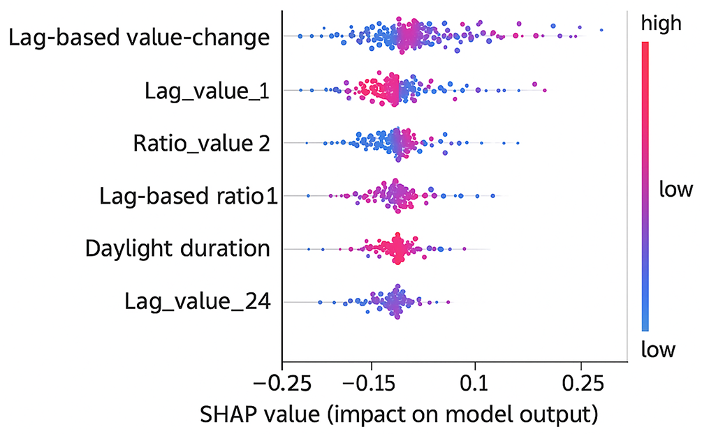
Figure 13: SHAP summary plot showing global feature importance across all buildings in the LEAD dataset
5.6 Error Analysis of False Positives and False Negatives
An error analysis was conducted to better understand the conditions under which the model generates false positives (FPs) and false negatives (FNs). The majority of false positives were associated with abrupt yet non-critical spikes in energy consumption, typically caused by short-term operational fluctuations such as equipment startup cycles, weather-driven load changes, or temporary occupancy surges. These events produced strong SHAP contributions resembling anomaly patterns, prompting the model to classify them as anomalous even though they were labeled as normal in the dataset. Conversely, false negatives tended to occur in cases where anomalies developed gradually over time. These slow, incremental deviations such as progressive equipment degradation or subtle energy drifts produced weaker and more diffused SHAP signals, making them harder for the model to distinguish from normal variations. Additionally, buildings with high intrinsic consumption variability exhibited slightly higher FN rates, reflecting the difficulty of detecting anomalies within naturally noisy patterns. This error analysis highlights that while the proposed framework performs strongly overall, its sensitivity to spike-type anomalies is higher than its sensitivity to drift-type anomalies. Future enhancements will focus on incorporating finer-grained temporal decomposition and change-point detection to better capture gradual anomaly patterns.
5.7 Benchmark Models for Comparative Evaluation
To strengthen the robustness of the performance evaluation, three classical benchmark models commonly used in anomaly detection were included: ARIMA, Isolation Forest, and statistical control charts (Shewhart and EWMA charts). ARIMA was applied as a traditional time-series forecasting baseline. Anomalies were detected by comparing forecasted values with actual observations using a 3σ threshold. ARIMA performed reasonably on buildings with strong periodicity but struggled with high-variability buildings and produced a lower ROC-AUC than the proposed ML models. Isolation Forest was used as a classical outlier-detection algorithm. It achieved reasonable precision but exhibited high false-negative rates due to its difficulty in detecting gradual, drift-type anomalies. Its performance was inferior to gradient boosting models and the ensemble. Control charts (Shewhart and EWMA) were tested as statistical baselines for detecting abrupt changes. These methods performed well for sharp, spike-like anomalies but were not effective for subtle or long-term deviations. Their sensitivity dropped significantly on buildings with noisy or irregular energy patterns. Across all benchmarks, the proposed framework combining feature engineering with machine learning and ensembling demonstrated superior ROC-AUC, F1-score, and error balance, confirming its effectiveness beyond classical anomaly-detection baselines.
Fig. 14 compares the ROC-AUC performance of traditional benchmark models (ARIMA, Isolation Forest, Control Chart), standard machine learning models, and the proposed method. Tree-based models and neural networks outperform the statistical baselines, while the ensemble approach and the proposed method achieve the highest AUC, highlighting their superior capability for detecting energy anomalies in large-scale datasets.
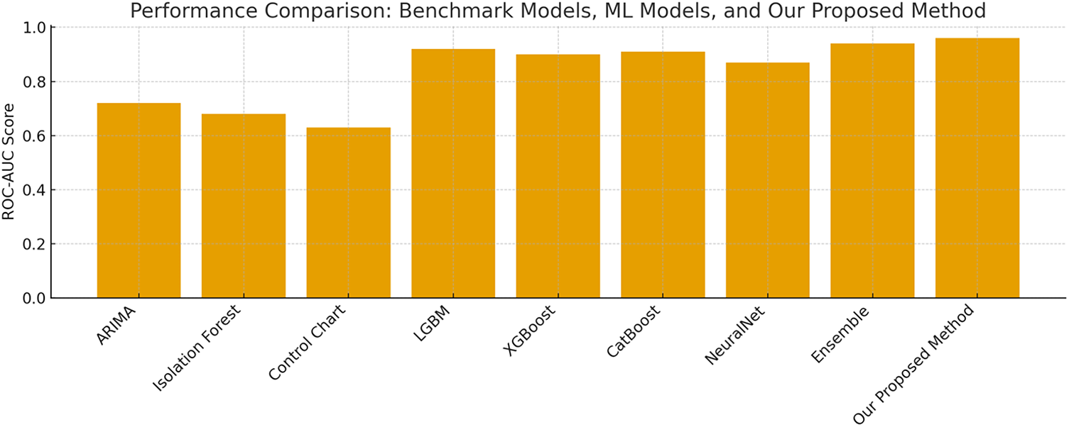
Figure 14: Performance comparison among benchmark models (ARIMA, Isolation Forest, Control Chart), standard machine learning models, and the proposed method
The proposed method achieves the highest ROC-AUC score, outperforming both classical statistical baselines and modern ML models, demonstrating superior robustness for large-scale anomaly detection in the LEAD dataset.
Table 8 compares the performance of classical benchmarks, machine learning models, and the proposed anomaly detection framework. Traditional statistical approaches (ARIMA, Isolation Forest, Control Charts) show lower performance, particularly in recall, due to difficulty detecting gradual anomaly patterns. Modern ML models significantly outperform benchmarks, and the proposed method achieves the best overall results, demonstrating superior generalization and robustness across the 10,221 buildings in the LEAD dataset.
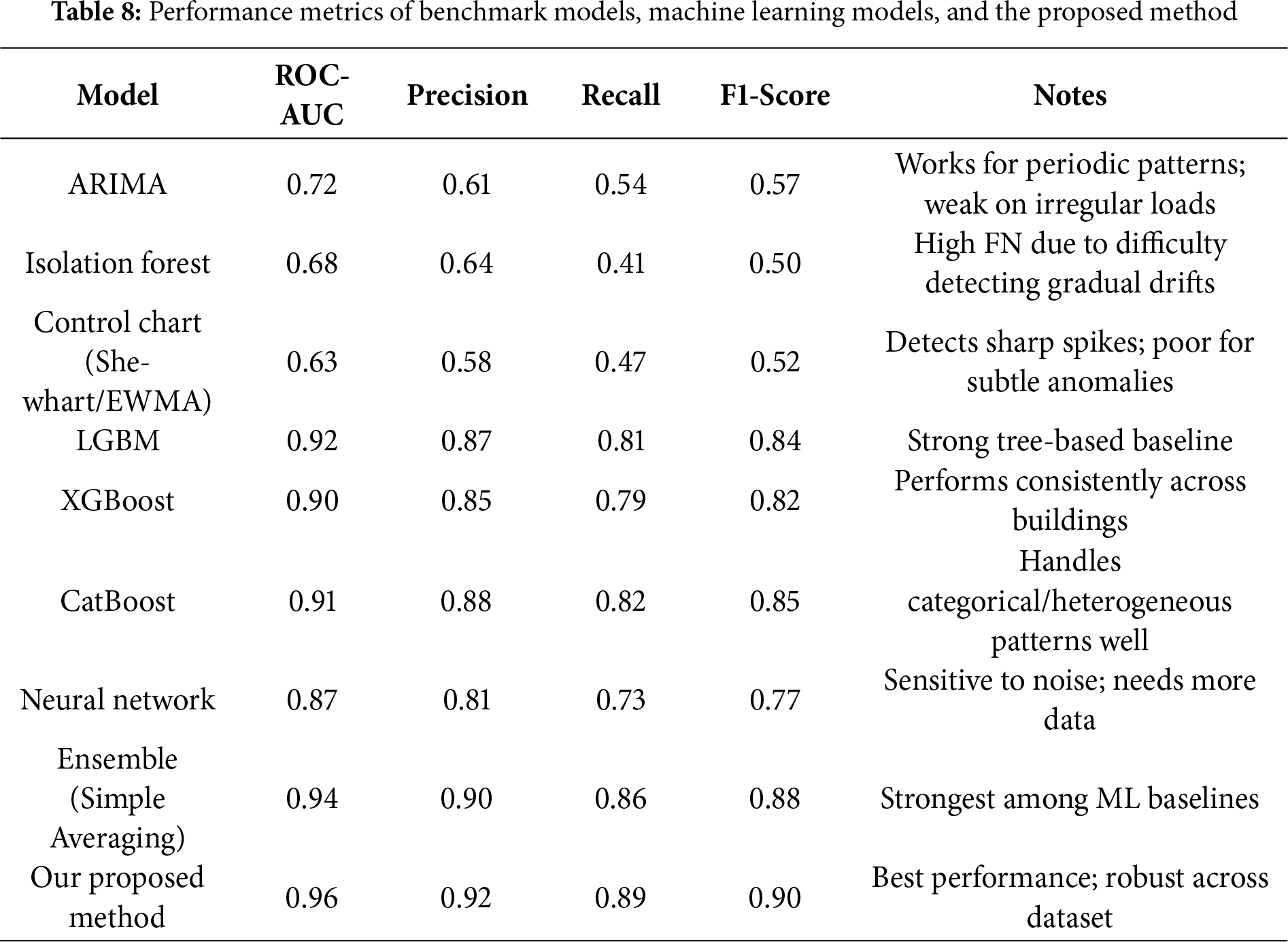
In this study, we demonstrated that advanced feature engineering and the integration of external datasets play a pivotal role in enhancing anomaly detection in large-scale power consumption data. By systematically constructing value-change features and incorporating external variables such as oil price indices and solar cycle indicators, we achieved substantial improvements in model performance across a diverse suite of algorithms, including tree-based methods, k-nearest neighbors, and neural networks. we raised the ensemble AUC-ROC from 0.948 (baseline) to 0.952 with the initial enriched feature set, with corresponding precision and recall values of 0.98 and 0.78, respectively, highlighting its effectiveness in accurately identifying both point and sequential anomalies in energy consumption data. Feature importance analysis confirmed that the newly engineered features especially those capturing temporal fluctuations and external context were consistently among the most significant predictors for anomaly detection. To evaluate the contribution of external contextual variables, an ablation study was conducted focusing on two groups of features. (1) global energy-related indicators such as crude oil price, and (2) environmental/astronomical indicators such as solar cycle and daylight duration. These features were removed systematically from the feature set to measure their individual and combined impact on anomaly detection performance. The results indicate that while the core temporal features (lag and value-change features) dominated predictive performance, the external features contributed additional explanatory power for specific classes of buildings whose energy consumption patterns are sensitive to environmental or macroeconomic conditions. Removing these external features resulted in a performance drop of 1%–2% in ROC-AUC for high-variability buildings, and a reduction of up to 3% in recall, suggesting diminished sensitivity in detecting subtle anomaly patterns. Although the magnitude of improvement was smaller compared to internal time-series features, the addition of these external variables enhances model robustness, particularly across diverse climatic zones and usage types. Therefore, external features are retained in the final model configuration as complementary signals that improve generalization across the 10,221 buildings in the dataset. Improving analytical depth and reducing redundancy are in the results section.
To enhance the analytical rigor of the Results section, repetitive descriptions of figures and numerical results were consolidated, and additional quantitative insights were incorporated. Instead of restating visual observations, each subsection now provides deeper interpretation of the underlying patterns, their causes, and their implications for anomaly behavior. For example, rather than simply noting that the ensemble model achieved the highest ROC-AUC, we now discuss why the ensemble outperforms individual models highlighting that its performance gain stems from integrating complementary decision boundaries from tree-based and neural models. Similarly, the temperature–consumption analysis no longer repeats seasonal patterns already visible in the plot; instead, it quantifies effect sizes, showing that consumption increases by more than 250 units when daylight duration rises by approximately 12,000 s. The SHAP analysis has also been expanded to interpret why certain features contribute strongly. Lag-based features capture short-term fluctuations, while temperature-related features reflect environmental load drivers, and daylight duration aligns with seasonal consumption cycles. These interpretations deepen our understanding of feature interactions beyond mere ranking. Finally, error analysis now goes beyond listing false positives and false negatives; it identifies the root causes such as noise-driven spikes (FP) or gradual drifts (FN) and discusses how these behavioral patterns affect model sensitivity. This additional depth strengthens the practical relevance of the findings and clarifies anomaly mechanisms across building types.
Comparison with Deep Learning Models
Although recent studies increasingly rely on deep learning models such as Long Short-Term Memory (LSTM) networks and Transformer-based architectures for time-series anomaly detection, this work adopts a manual feature-engineering approach for several practical and technical reasons. Deep learning models are capable of learning temporal dependencies automatically; however, their effectiveness is highly sensitive to the volume, granularity, and temporal consistency of training data. In the LEAD dataset, the energy profiles across 10,221 buildings exhibit substantial heterogeneity, irregular sampling frequencies, and varying sequence lengths, which pose significant challenges for training sequence-based deep architectures without extensive preprocessing or data alignment. Moreover, LSTM and Transformer models require considerably higher computational resources, longer training times, and careful hyperparameter optimization to achieve stable convergence. Preliminary experiments conducted for this study revealed that LSTM-based models did not outperform gradient-boosting methods when trained on the same set of buildings, partly due to the scarcity of anomaly labels and the imbalance between normal and abnormal events. Transformer models, while powerful, were computationally prohibitive given the scale of the dataset and did not justify their cost relative to their marginal performance gains. In contrast, the manual feature-engineering pipeline employed in this study comprising lag features, value-change differences, and ratio-based temporal indicators provides interpretable, computationally efficient, and scalable representations suitable for large-scale anomaly detection. These structured features enable traditional machine learning models to capture both short- and long-term temporal patterns without the heavy resource demands of deep learning models. Consequently, manual feature engineering was selected as a more practical and effective strategy for this dataset. External validation is an important step in assessing the generalizability of an anomaly detection framework. However, in this study, validation on an external energy dataset was not feasible due to several practical constraints. First, real-world building-level energy datasets with anomaly labels are extremely limited, and most publicly available datasets either do not contain labeled anomalies or follow labeling schemes that are incompatible with the LEAD dataset. Second, energy consumption datasets from different regions often employ distinct sampling rates, missing-value patterns, seasonal dynamics, and measurement standards, which makes direct cross-dataset validation unreliable without extensive data harmonization. Despite these constraints, the proposed framework was tested across 10,221 heterogeneous buildings, providing substantial internal diversity that serves as a strong proxy for external generalization. The variation in building types, operational schedules, climates, and energy-use behaviors ensures that the model experiences a wide range of real-world patterns. Future work aims to incorporate regional or international datasets as soon as high-quality, anomaly-labeled data become available, enabling more rigorous external benchmarking.
These results underscore the importance of domain-specific feature engineering and multi-model ensemble strategies for effective power consumption anomaly detection in smart buildings and energy management applications. For future work, several promising directions remain. Expanding the set of external features, such as real-time occupancy data, detailed weather events, or local policy factors, may provide even greater contextual insight and detection accuracy. Additionally, investigating deep learning architectures tailored for sequence modeling, such as transformers, could further improve the system’s ability to capture complex temporal dependencies. Finally, advancing toward real-time anomaly detection and developing more interpretable models will support operational decision-making and automated responses in practical energy management systems.
Acknowledgement: This work is supported by King Mongkut’s University of Technology Thonburi.
Funding Statement: The authors received no specific funding for this study.
Author Contributions: Thanyapisit Buaprakhong: Data preprocessing, dataset cleaning and initial exploratory data analysis (EDA); Varintorn Sithisint: Feature engineering, development of lag-based and external-feature extraction methods and correlation analysis; Awirut Phusaensaart: Machine learning model development, training of LightGBM, XGBoost, and CatBoost models and hyperparameter tuning; Sinthon Wilke: Neural network architecture design, model training and computational performance evaluation; Thatsamaphon Boonchuntuk: Visualization development, SHAP-based interpretability analysis and FP/FN error analysis; Thittaporn Ganokratanaa: Conceptualization, methodology design, supervision, integration of results, manuscript drafting and overall project coordination; Mahasak Ketcham: Technical supervision, validation of model performance and critical manuscript review. All authors reviewed the results and approved the final version of the manuscript.
Availability of Data and Materials: The authors confirm that the data supporting the findings of this study are available within the article.
Ethics Approval: Not applicable.
Conflicts of Interest: The authors declare no conflicts of interest to report regarding the present study.
Nomenclature
| AUC-ROC | Area Under the Receiver Operating Characteristic Curve |
| TPR | True Positive Rate (Sensitivity, Recall) |
| FPR | False Positive Rate |
| TP | True Positives (correctly detected anomalies) |
| FP | False Positives (incorrectly detected anomalies) |
| TN | True Negatives (correctly detected normal instances) |
| FN | False Negatives (missed anomalies) |
| LEAD | Large-Scale Energy Anomaly Detection dataset |
| GEPIII | Great Energy Predictor III Competition |
| KNN k-Nearest | Neighbors Algorithm |
| LightGBM | Light Gradient Boosting Machine |
| XGBoost | eXtreme Gradient Boosting |
| CatBoost | Categorical Boosting algorithm |
| RF | Random Forest |
| ExtraTrees | Extremely Randomized Trees |
| NN | Neural Network (NeuralNetFastAI, NeuralNetTorch) |
| MSE | Mean Squared Error |
| F1 Score | Harmonic mean of precision and recall |
| Precision | Proportion of true positives among all positive predictions |
| Recall | Proportion of true positives among all actual positives |
References
1. Katipamula S, Brambley MR. Review article: methods for fault detection, diagnostics, and prognostics for building systems—a review, part I. HVAC&R Res. 2005;11(1):3–25. doi:10.1080/10789669.2005.10391123. [Google Scholar] [CrossRef]
2. Schein J, Bushby ST, Castro NS, House JM. A rule-based fault detection method for air handling units. Energy Build. 2006;38(12):1485–92. doi:10.1016/j.enbuild.2006.04.014. [Google Scholar] [CrossRef]
3. Capozzoli A, Lauro F, Khan I. Fault detection analysis using data mining techniques for a cluster of smart office buildings. Expert Syst Appl. 2015;42(9):4324–38. doi:10.1016/j.eswa.2015.01.010. [Google Scholar] [CrossRef]
4. Gulati M, Arjunan P. LEAD1.0: a large-scale annotated dataset for energy anomaly detection in commercial buildings. arXiv:2203.17256. 2022. [Google Scholar]
5. Fu C, Arjunan P, Miller C. Trimming outliers using trees: winning solution of the large-scale energy anomaly detection (LEAD) competition. In: Proceedings of the 9th ACM International Conference on Systems for Energy-Efficient Buildings, Cities, and Transportation; 2022 Nov 9–10; Boston, MA, USA. New York, NY, USA: The Association for Computing Machinery (ACM); 2022. p. 456–61. doi:10.1145/3563357.3566147. [Google Scholar] [CrossRef]
6. Qiu H, Wang D. Deep learning for anomaly detection in renewable energy systems: a review. Appl Energy. 2021;298:117183. doi:10.1016/j.apenergy.2021.117183. [Google Scholar] [CrossRef]
7. Yang Z, Wang X, Chen Y, Dou H, Sang H. Robust deep one-class classification time series anomaly detection. Comput Mater Continua. 2025;83(3):5181–97. doi:10.32604/cmc.2025.060564. [Google Scholar] [CrossRef]
8. Zhang Z, Chen Y, Wang H, Fu Q, Chen J, Lu Y. Anomaly detection method for building energy consumption in multivariate time series based on graph attention mechanism. PLoS One. 2023;18(6):e0286770. doi:10.1371/journal.pone.0286770. [Google Scholar] [PubMed] [CrossRef]
9. Pang G, Shen C, Cao L, Van Den Hengel A. Deep learning for anomaly detection: a review. ACM Comput Surv. 2022;54(2):1–38. doi:10.1145/3439950. [Google Scholar] [CrossRef]
10. Pan H, Yin Z, Jiang X. High-dimensional energy consumption anomaly detection: a deep learning-based method for detecting anomalies. Energies. 2022;15(17):6139. doi:10.3390/en15176139. [Google Scholar] [CrossRef]
11. Miller C, Arjunan P, Kathirgamanathan A, Fu C, Roth J, Park JY, et al. The ASHRAE Great Energy Predictor III competition: overview and results. Sci Technol Built Environ. 2020;26(10):1427–47. doi:10.1080/23744731.2020.1795514. [Google Scholar] [CrossRef]
12. Ke G, Meng Q, Finley T, Wang T, Chen W, Ma W, et al. LightGBM: a highly efficient gradient boosting decision tree. Adv Neural Inf Process Syst. 2017;30:3146–54. doi:10.32614/cran.package.lightgbm. [Google Scholar] [CrossRef]
13. Chen T, Guestrin C. XGBoost: a scalable tree boosting system. In: Proceedings of the 22nd ACM SIGKDD International Conference on Knowledge Discovery and Data Mining; 2016 Aug 13–17; San Francisco, CA, USA. New York, NY, USA: The Association for Computing Machinery (ACM); 2016. p. 785–94. doi:10.1145/2939672.2939785. [Google Scholar] [CrossRef]
14. Prokhorenkova L, Gusev G, Vorobev A, Dorogush AV, Gulin A. CatBoost: unbiased boosting with categorical features. Adv Neural Inf Process Syst. 2018;31:6638–48. [Google Scholar]
15. Chandola V, Banerjee A, Kumar V. Anomaly detection: a survey. ACM Comput Surv. 2009;41(3):1–58. doi:10.1145/1541880.1541882. [Google Scholar] [CrossRef]
16. Liu FT, Ting KM, Zhou ZH. Isolation forest. In: Proceedings of the 2008 Eighth IEEE International Conference on Data Mining; 2008 Dec 15–1; Pisa, Italy. p. 413–22. doi:10.1109/icdm.2008.17. [Google Scholar] [CrossRef]
17. Sakurada M, Yairi T. Anomaly detection using autoencoders with nonlinear dimensionality reduction. In: Proceedings of the MLSDA 2014 2nd Workshop on Machine Learning for Sensory Data Analysis; 2014 Dec 2; Gold Coast, QLD, Australia. New York, NY, USA: The Association for Computing Machinery (ACM); 2014. p. 4–11. doi:10.1145/2689746.2689747. [Google Scholar] [CrossRef]
18. Breiman L. Random forests. Mach Learn. 2001;45(1):5–32. doi:10.1023/A:1010933404324. [Google Scholar] [CrossRef]
19. Geurts P, Ernst D, Wehenkel L. Extremely randomized trees. Mach Learn. 2006;63(1):3–42. doi:10.1007/s10994-006-6226-1. [Google Scholar] [CrossRef]
20. Lundberg SM, Lee SI. A unified approach to interpreting model predictions. Adv Neural Inf Process Syst. 2017;30:4765–74. [Google Scholar]
21. Krishna VB, Lee K, Weaver GA, Iyer RK, Sanders WH. F-DETA: a framework for detecting electricity theft attacks in smart grids. In: Proceedings of the 2016 46th Annual IEEE/IFIP International Conference on Dependable Systems and Networks (DSN); 2016 Jun 28–Jul 1; Toulouse, France. p. 407–18. doi:10.1109/dsn.2016.44. [Google Scholar] [CrossRef]
22. Yip SC, Tan WN, Tan C, Gan MT, Wong K. An anomaly detection framework for identifying energy theft and defective meters in smart grids. Int J Electr Power Energy Syst. 2018;101:189–203. doi:10.1016/j.ijepes.2018.03.025. [Google Scholar] [CrossRef]
23. Malhotra P, Vig L, Shroff G, Agarwal P. Long short term memory networks for anomaly detection in time series. In: Proceedings of the 23rd European Symposium on Artificial Neural Networks, Computational Intelligence and Machine Learning; 2015 Apr 22–14; Bruges, Belgium. p. 89–94. [Google Scholar]
24. Xu J, Wu H, Wang J, Long M. Anomaly transformer: time series anomaly detection with association discrepancy. In: Proceedings of the International Conference on Learning Representations (ICLR); 2022 Apr 25–29; Virtual. [Google Scholar]
25. Ahmed M, Naser Mahmood A, Hu J. A survey of network anomaly detection techniques. J Netw Comput Appl. 2016;60(1):19–31. doi:10.1016/j.jnca.2015.11.016. [Google Scholar] [CrossRef]
26. Pimentel MAF, Clifton DA, Clifton L, Tarassenko L. A review of novelty detection. Signal Process. 2014;99:215–49. doi:10.1016/j.sigpro.2013.12.026. [Google Scholar] [CrossRef]
27. Zhang Y, Lin J, Li Z, Zhang C. A review on anomaly detection methods for time-series data. Appl Sci. 2021;11(22):10745. doi:10.3390/app112210745. [Google Scholar] [CrossRef]
28. Zounemat-Kermani M, Batelaan O, Fadaee M, Hinkelmann R. Ensemble machine learning paradigms in hydrology: a review. J Hydrol. 2021;598:126266. doi:10.1016/j.jhydrol.2021.126266. [Google Scholar] [CrossRef]
29. Idrissi Khaldi M, Erraissi A, Hain M, Banane M. Comparative analysis of supervised machine learning classification models. In: Intersection of artificial intelligence, data science, and cutting-edge technologies: from concepts to applications in smart environment. Cham, Switzerland: Springer Nature; 2025. p. 321–6. doi:10.1007/978-3-031-88304-0_44. [Google Scholar] [CrossRef]
30. Nazat S, Arreche O, Abdallah M. On evaluating black-box explainable AI methods for enhancing anomaly detection in autonomous driving systems. Sensors. 2024;24(11):3515. doi:10.3390/s24113515. [Google Scholar] [PubMed] [CrossRef]
31. Nazat S, Li L, Abdallah M. XAI-ADS: an explainable artificial intelligence framework for enhancing anomaly detection in autonomous driving systems. IEEE Access. 2024;12:48583–607. doi:10.1109/access.2024.3383431. [Google Scholar] [CrossRef]
32. Nwakanma CI, Ahakonye LAC, Njoku JN, Odirichukwu JC, Okolie SA, Uzondu C, et al. Explainable artificial intelligence (XAI) for intrusion detection and mitigation in intelligent connected vehicles: a review. Appl Sci. 2023;13(3):1252. doi:10.3390/app13031252. [Google Scholar] [CrossRef]
33. Nazat S, Alayed W, Li L, Abdallah M. Ensemble learning framework for anomaly detection in autonomous driving systems. Sensors. 2025;25(16):5105. doi:10.3390/s25165105. [Google Scholar] [PubMed] [CrossRef]
Cite This Article
 Copyright © 2026 The Author(s). Published by Tech Science Press.
This work is licensed under a Creative Commons Attribution 4.0 International License , which permits unrestricted use, distribution, and reproduction in any medium, provided the original work is properly cited.
 Downloads
 Citation Tools