
 Submit a Paper
 Propose a Special lssue
 Open Access
ARTICLE

Improved Gain Shared Knowledge Optimizer Based Reactive Power Optimization for Various Renewable Penetrated Power Grids with Static Var Generator Participation
1 Yunnan Power Grid Co., Ltd., Kunming Power Supply Bureau, Kunming, 650000, China
2 Yunnan Power Dispatching and Control Center, Kunming, 650000, China
3 Faculty of Electric Power Engineering, Kunming University of Science and Technology, Kunming, 650500, China
* Corresponding Author: Bo Yang. Email:
(This article belongs to the Special Issue: Grid Integration of Intermittent Renewable Energy Resources: Technologies, Policies, and Operational Strategies)
Energy Engineering 2026, 123(3), 2 https://doi.org/10.32604/ee.2025.071166
Received 01 August 2025; Accepted 05 October 2025; Issue published 27 February 2026
 View Full Text
 Download PDF
Abstract
An optimized volt-ampere reactive (VAR) control framework is proposed for transmission-level power systems to simultaneously mitigate voltage deviations and active-power losses through coordinated control of large-scale wind/solar farms with shunt static var generators (SVGs). The model explicitly represents reactive-power regulation characteristics of doubly-fed wind turbines and PV inverters under real-time meteorological conditions, and quantifies SVG high-speed compensation capability, enabling seamless transition from localized VAR management to a globally coordinated strategy. An enhanced adaptive gain-sharing knowledge optimizer (AGSK-SD) integrates simulated annealing and diversity maintenance to autonomously tune voltage-control actions, renewable source reactive-power set-points, and SVG output. The algorithm adaptively modulates knowledge factors and ratios across search phases, performs SA-based fine-grained local exploitation, and periodically re-injects population diversity to prevent premature convergence. Comprehensive tests on IEEE 9-bus and 39-bus systems demonstrate AGSK-SD’s superiority over NSGA-II and MOPSO in hypervolume (HV), inverse generative distance (IGD), and spread metrics while maintaining acceptable computational burden. The method reduces network losses from 2.7191 to 2.15 MW (20.79% reduction) and from 15.1891 to 11.22 MW (26.16% reduction) in the 9-bus and 39-bus systems respectively. Simultaneously, the cumulative voltage-deviation index decreases from 0.0277 to 3.42 × 10⁻⁴ p.u. (98.77% reduction) in the 9-bus system, and from 0.0556 to 0.0107 p.u. (80.76% reduction) in the 39-bus system. These improvements demonstrate significant suppression of line losses and voltage fluctuations. Comparative analysis with traditional heuristic optimization algorithms confirms the superior performance of the proposed approach.Keywords
Rapid economic growth and rising living standards have steadily increased electricity demand, which is essential for social development [1–3]. However, environmental degradation and the deepening energy crisis are accelerating the transition to renewable energy for cleaner power generation [4–7]. While large-scale wind and solar technologies have strengthened supply capacity, they also introduce critical challenges [8]. Their inherent variability creates uncertainty that threatens system stability [9,10]. Furthermore, their fluctuating output reshapes traditional network topologies and redistributes power flows [11–13]. Consequently, issues such as voltage deviations and increased losses have become more pronounced [14].
Reactive-power optimization for renewable-energy grid connection (REGC) has become a vibrant research frontier [15–17]. Early work concentrated on single-objective optimization (SOO) that incorporated wind or photovoltaic (PV) generation, seeking to cut operating costs, boost renewable utilization, and curb voltage deviations, with tailored models developed accordingly [18–20]. Reference [21] introduces an enhanced particle-swarm scheme to lower active-power losses and improve voltage profiles. Reference [22] blends particle swarm optimization (PSO) with the pathfinder algorithm to dispatch reactive power with the same loss-minimization goal. Reference [23] formulates a mixed-integer nonlinear program (MINLP) to minimize voltage deviation, thereby stabilizing nodal voltages and enhancing overall performance. As renewable penetration deepens and system complexity grows, SOO has gradually given way to multi-objective optimization (MOO) to better tackle the multifaceted demands of modern power-system operation.
Integrating wind and other renewables into reactive-power control creates a complex optimization task. Like its conventional-grid counterpart, this task is nonlinear, non-convex, and entangled with discrete variables. Reference [24] formulates a multi-objective model for distribution networks with large shares of wind, solar, and electric vehicles (EV). This model seeks to cut losses and voltage deviations while also enlarging the static voltage-stability margin. Adding compensators boosts stability, yet may marginally raise losses and voltage excursions. Reference [25] applies multi-objective particle-swarm optimization (MOPSO) to coordinate reactive power, aiming for both stability and cost minimization, but its effectiveness under highly dynamic grid conditions remains limited. Reference [26] adopts mixed-integer convex programming (MICP), relaxing line-current models and convexifying discrete variables; although accurate, the approach is computationally heavy. Reference [27] merges genetic search with an interior-point routine (GIPA) to handle wind-farm involvement, yet the heuristic algorithm (HA) risks local optima. Collectively, existing algorithms struggle to adapt to fast-changing operating states and to fully harness renewable sources’ reactive capability, while their computational efficiency still falls short of real-time needs.
To overcome the aforementioned problems, this work first constructs a comprehensive mathematical model for grid reactive power optimization and regulation. This model incorporates wind farms, PV power plants, and reactive power optimization devices. The problem is addressed using the adaptive gain shared knowledge with simulated annealing (SA) and diversity maintenance (AGSK-SD). The AGSK-SD optimization algorithm is a new and improved gain shared knowledge (GSK) algorithm, which effectively improves both optimization accuracy and efficiency. It avoids convergence to local optima by adaptively adjusting knowledge factors (KF) and knowledge ratios (KR), introducing simulated annealing and local search mechanisms, and enhancing population deiversity. In this work, the optimization mechanisms are described in detail, along with the specific design of the reactive power optimization framework. Next, the effectiveness of a static var generator (SVG) is verified through simulation experiments. Finally, the performance of the proposed method is further validated by introducing wind and solar energy into the extended IEEE 9-bus and 39-bus standard systems, and conducting simulation tests and penetration analysis using comparative algorithms. This study mainly focuses on reactive power optimization in the transmission grid, solving the challenges brought by the integration of wind and solar power plants through the transmission grid.
The main contributions of this work are as follows:
(1) This paper proposes a unified multi-objective optimization model that simultaneously incorporates the real-time adjustable reactive-power margins of wind turbines, PV inverters, and SVGs.
(2) The GSK framework introduces a dynamic control mechanism of “Adaptive KF + KR”: This mechanism automatically adjusts the search step size according to the iteration stage, allowing the algorithm to rapidly converge toward the optimal region in the early stage and refine local optima during the later stage, thus improving the local search accuracy;
(3) Simulated annealing based fine search and diversity perturbation mechanisms are deeply coupled in GSK: The annealing mechanism enables probabilistic escape from local optima, while the diversity perturbation periodically re-expands the solution space. These two strategies operate synergistically to simultaneously improve global convergence and the quality of the Pareto front in terms of uniformity and diversity.
Although the optimization model extension of integrating SVG reactive power capability into renewable dominant grid is considered for completeness, the main novelty lies in the algorithm improvement: the proposed adaptive parameter adjustment, simulated annealing coupling, and diversity enhancement mechanism are the theoretical breakthroughs of this paper.
2 Reactive Power Optimization Model of the Power Grid with SVG Considering Wind-Solar New Energy Access
Reactive power models for wind and PV plants are central to any voltage–support strategy in renewable-rich grids. The wind-based model schedules the farms’ reactive output to strengthen voltage stability, whereas the PV-based model adjusts the plants’ reactive injection to enhance voltage quality. Coupled with SVGs, these controls curb losses, raise transfer limits, and safeguard secure, cost-effective operation under high renewable penetration. The optimization pursues minimal active-power loss and voltage deviation while respecting operational limits: node-voltage bands, line-current ceilings, and the reactive range of wind and PV units. Recent studies, such as reference [28], corroborate that centralized coordination of wind, PV and SVG reactive resources can markedly elevate renewable-hosting capacity, further underscoring the necessity of the integrated optimization framework proposed herein.
2.1 Reactive Power Regulation Model of PV Power System
During the operation of a PV power plant, its active power output level is mainly limited by the real-time environmental conditions, especially the coupling effect of solar irradiance and ambient temperature. When the power plant adopts an optimal control strategy based on maximum power point tracking (MPPT), its theoretical active output can be accurately modeled by [29]
where
According to the operating characteristics of a PV power plant, the adjustable range of its reactive power output is mainly limited by two key factors: the real-time active power output level of the plant, and the maximum rated capacity of the grid-connected inverter. This relationship is expressed as follows [30]:
where
2.2 Reactive Power Regulation Model of Wind Power System
This study takes the doubly-fed induction generator as the representative unit for a detailed investigation of wind-turbine reactive-power control [31]. Fig. 1 depicts the adopted structure, where both the mechanical input
where
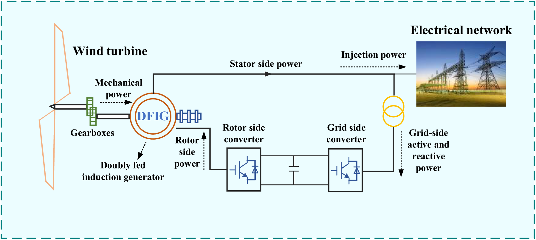
Figure 1: The energy transformation mechanism in doubly-fed induction generators
The span of the turbine’s reactive-power adjustment window is governed by the individual limits of the stator-side and grid-side converters, expressed as follows [32]:
where
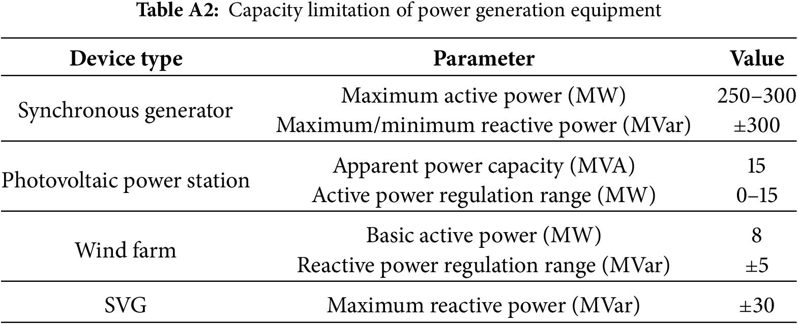
In this case, the maximum stator-side current constraints and grid-side converter capacity limits are shown in Appendix A. Based on this, when the current wind speed conditions are known, the reactive power output regulation range of a single wind turbine can be further extrapolated and extended to the whole wind farm level to determine the aggregate reactive power output adjustable range of the entire wind farm.
Voltage-source SVGs are widely adopted for high-speed reactive power optimization. As shown in Fig. A1 (Appendix B), the converter bridge is shunt-connected to the grid via a coupling reactor and a DC-link capacitor. The loss equivalent circuit diagram is shown in Fig. A2 (Appendix B). By regulating the magnitude and phase of the converter AC-side voltage
where
With the integration of wind farms into the power grid, it is common practice to install corresponding reactive power optimization equipment to mitigate potential instability in the bus voltage caused by imbalances in reactive power. Although doubly-fed wind turbines possess a certain capacity for reactive power regulation, their performance is generally inferior to that of SVGs. Therefore, the incorporation of SVGs is essential to enhance the system’s reactive power optimization.
As shown in Fig. 2, the mathematical models of PV, wind and SVG are systematically integrated into a unified reactive power optimisation framework, which presents a closed-loop logic from resource parameter input, equipment capability portrayal to global collaborative decision-making.
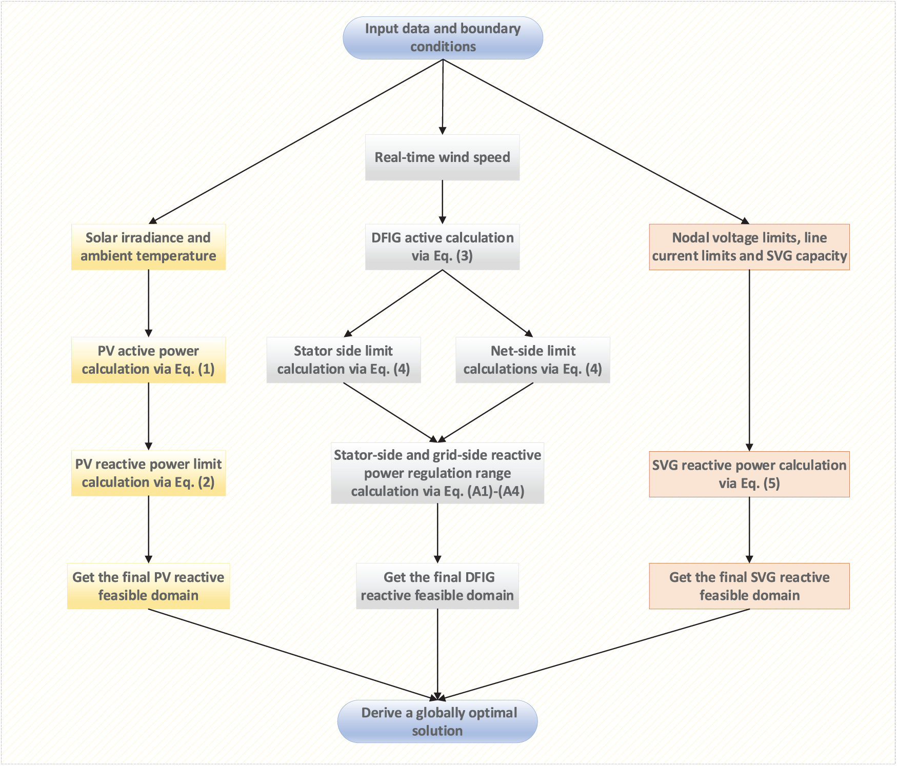
Figure 2: Integrated flowchart of the mathematical model for PV, wind and SVG systems
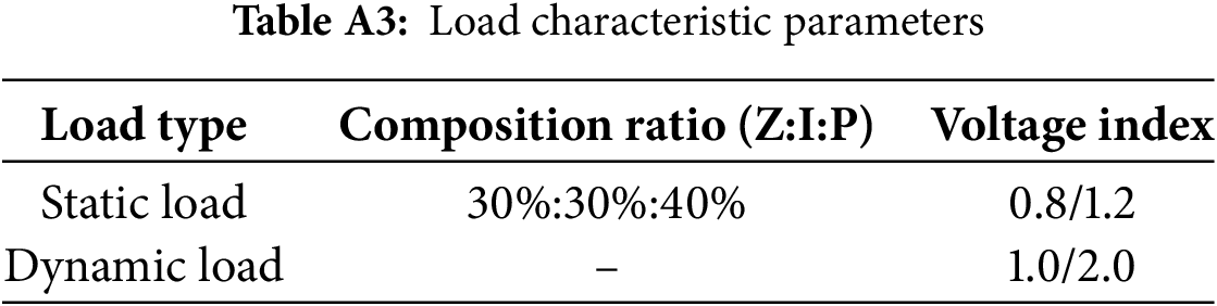
2.4 Load Modelling Extensions for High R/X Distribution Networks
Due to the high R/X ratios in the distribution network, the node voltage varies significantly with the fluctuation of load and renewable energy output, and the traditional PQ model is no longer applicable. For this reason, this paper introduces a combination of ZIP load model and exponential load model into the original optimization framework to portray the load dependence on the nodal voltage.
The load is decomposed into three parts, constant impedance (Z), constant current (I) and constant power (P), and its active and reactive power can be expressed as:
where
Embedding the above expression directly into the node power balance constraints of the existing optimization model, i.e.:
where
For voltage sensitive loads, the exponential form is used as:
where the indices
The power balance constraint for this model is:
where
The constructed reactive power optimization model aims to minimize line losses and voltage deviations in the grid transmission process, which is formulated as follows [33]:
where
The formalization of the objective vector and dominance relationship is as follows. According to the dual objective optimization problem defined above, the objective vector can be formally expressed as:
The dominance relationship adopts the Pareto dominance criterion: for any two solutions
In the context of grid reactive power optimization involving wind and solar energy participation in regulation and control, a series of equality and inequality constraints need to be simultaneously satisfied to ensure the practical feasibility of the optimization scheme. These constraints are formulated as follows [34]:
1. Power-flow equation constraints
where
2. Generator constraints
where
3. Reactive power optimization device SVG and transformer tap constraints
where
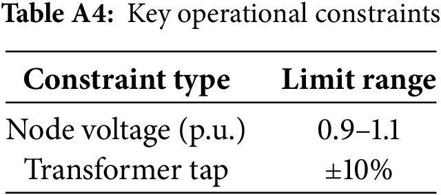
4. Safety constraint
Node i’s voltage must stay between
3 AGSK-SD Optimizer Design for Reactive Power Optimization
3.1 Introduction to GSK Algorithm
The GSK optimization algorithm is a group-based optimization method inspired by the human process of acquiring and sharing knowledge. In reactive power optimization, GSK algorithm operates by mimicking the knowledge acquisition and sharing behaviors among individuals in a group. Through this imitation process, the algorithm aims to optimize the objective function, thereby achieving reactive power optimization.
To establish a comprehensive foundation for our enhanced algorithm, we first describe the standard GSK framework, which provides the basis for our subsequent modifications.
Assume that the fitness vector of the ith individual is denoted as
In the primary knowledge acquisition and sharing stage as well as the advanced knowledge acquisition and sharing stage, the number of human individuals in the primary and advanced dimensions changes dynamically over time, as shown in the lower right subplot of Fig. 3. To address this phenomenon, GSK algorithm quantitatively describes this dynamic process of change in the number of primary and advanced dimensions in the mathematical form presented in Eqs. (22) and (23), respectively [35].
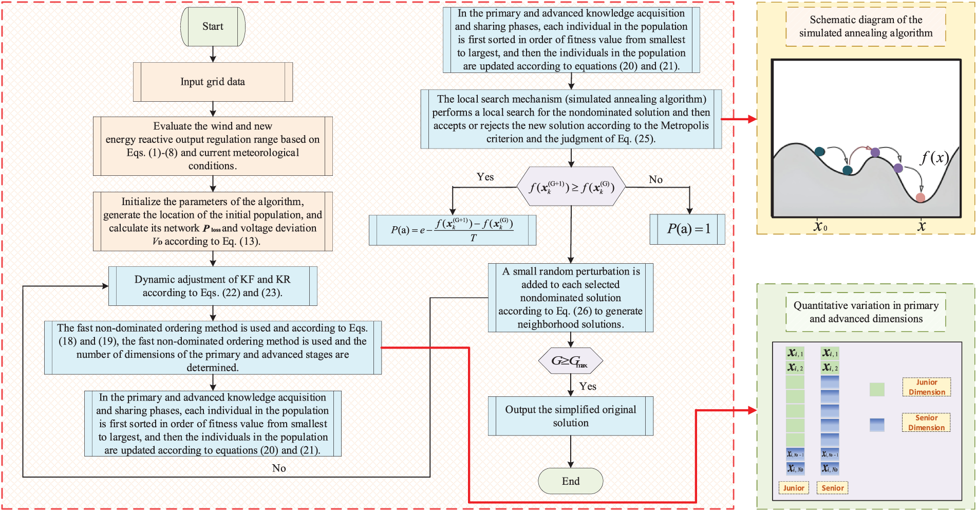
Figure 3: Flowchart of AGSK-SD algorithm, highlighting the adaptive knowledge factor adjustment, simulated annealing local search, and diversity perturbation mechanisms that enhance global convergence
Building upon this foundation, we now introduce the specific optimization strategies that distinguish our enhanced approach from the standard GSK framework.
where
As the iterations, the number of dimensions in the primary stage shows a decreasing trend, while the number of dimensions in the advanced stage shows an increasing trend. In the primary knowledge acquisition and sharing stage, each individual in the population is updated by [36]
where
Advanced stage can be updated as follows [37]:
where
3.2 Optimization Strategies for GSK Algorithm
3.2.1 Adaptive Parameter Tuning
In the realm of reactive power optimization, GSK algorithm demonstrates strong adaptability across various optimization stages through the dynamic modulation of KF and KR. During the initial phase of the optimization process, setting relatively large values for both KF and KR enables the algorithm to quickly locate regions near the global optimum, thereby laying a solid foundation for subsequent fine-tuning. As the optimization progresses into later stages, it becomes essential to gradually decrease the values of KF and KR. This strategic adjustment enhances the algorithm’s precision during local search operations, effectively reducing the risk of premature convergence to local optima and promoting a more comprehensive exploration of the solution space to identify the global optimal solution.
To complement the adaptive parameter tuning mechanism, we incorporated a simulated annealing local search strategy to further enhance the algorithm’s exploitation capabilities.
The dynamic adjustment for KF is described as follows:
where
The dynamic adjustment for KR is expressed as follows:
where
In each iteration, a refined hybrid scheme boosts solution quality and convergence. Selected non-dominated individuals are subjected to a focused Simulated Annealing (SA) local search, leveraging temperature-driven probabilistic moves to escape local optima while still exploring promising regions. This local/global synergy—illustrated in the inset of Fig. 3—raises accuracy and robustness without appreciably adding computation, delivering a superior final solution.
SA emulates the physical annealing process: the system is slowly cooled from high to low temperature to locate the global optimum while avoiding local traps. The cooling schedule is defined as [38]:
where
While the simulated annealing mechanism addresses local search intensification, we recognized the need for an additional diversity preservation strategy to maintain population variety throughout the optimization process.
In SA algorithm, the acceptance criterion usually uses the Metropolis criterion. Assuming that the current solution is
where
To enhance the global search capability and reduce the risk of falling into local optimal solutions, a diversity enhancement mechanism is introduced. Specifically, by dynamically injecting controllable random perturbation factors into the search process, the system can periodically deviate from the current search trajectory, thus effectively expanding the exploration range of the solution space.
For each selected non-dominated solution
where
The range of the randomized perturbation ϵ can be adjusted according to the size and complexity of the problem. Typically,
where
3.3 Application of AGSK-SD Algorithm in Reactive Power Optimization
To further clarify the novelty and advancement of the proposed AGSK-SD algorithm, a comparative analysis with the original GSK framework and its other variants is provided. While the standard GSK algorithm introduces a valuable metaphor for knowledge acquisition and sharing, it often suffers from premature convergence and an imbalance between exploration and exploitation when tackling complex multimodal problems such as reactive power optimization.
The selection of these specific enhancement strategies was guided by the unique challenges presented by reactive power optimization problems, which require careful balancing between global exploration and local exploitation capabilities.
The key innovations of AGSK-SD that differentiate it from earlier GSK frameworks are threefold, as summarized in Table 1.
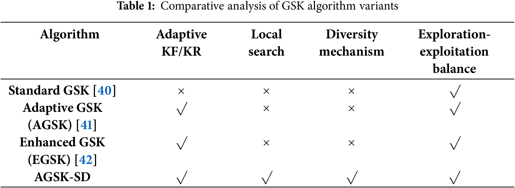
(1) Adaptive core mechanism: Unlike standard GSK and many of its variants that rely on static parameters, AGSK-SD introduces a dynamic adaptive mechanism for both the KF and KR. This allows the algorithm to autonomously shift its behavior from global exploration to local exploitation as the optimization progresses, significantly enhancing search efficiency and final solution quality.
(2) Synergistic hybrid strategy: While SA or diversity maintenance strategies have been used independently in other metaheuristics, their deep integration into the GSK lifecycle is novel. In AGSK-SD, SA is not a standalone post-processor but is selectively applied to non-dominated solutions, acting as a refined local search tool. This is seamlessly coupled with the global search phases of GSK.
(3) Problem-specific design: The design of the diversity perturbation mechanism is specifically tailored for the characteristics of power system optimization problems (e.g., variable bounds, discrete-continuous mixed variables), ensuring that the perturbations are both effective and efficient within the feasible solution space.
This comprehensive integration of adaptive mechanisms, local search intensification, and diversity preservation strategies transforms the GSK framework into a specialized tool specifically designed for the complexities of modern power system optimization.
This multi-faceted enhancement transforms the GSK from a robust general-purpose optimizer into a highly specialized and powerful algorithm for handling the intricacies of reactive power optimization in modern power grids.
The proposed AGSK-SD algorithm, therefore, represents a significant evolution of the GSK framework by moving beyond parameter adaptation to a strategic hybridization, where adaptive control, targeted local search, and managed diversity work in concert to address the specific challenges of non-convex, constrained, multi-objective optimization problems found in renewable-penetrated power systems.
Conventional heuristics often converge prematurely and yield poorly distributed Pareto fronts for multi-objective reactive-power optimization. To overcome these drawbacks, this paper employs AGSK-SD, an enhanced GSK variant. AGSK-SD adaptively tunes KF and KR across the search phases—speeding up early exploration and refining late-stage exploitation. A cyclic SA search further polishes selected individuals, markedly raising solution quality. Random perturbations are injected to sustain diversity, deter stagnation, and bolster global search. Together, these refinements boost efficiency, robustness, and practical applicability for complex multi-objective tasks; the overall procedure is outlined in Fig. 3.
In this study, based on the MATLAB simulation platform, the performance of the proposed AGSK-SD algorithm in power system reactive power optimization is systematically verified. The extended IEEE 9-bus and 39-bus standard test systems are utilized for validation (see Figs. 4 and 5 for details of the system topology and the location of the scenery-SVG access).
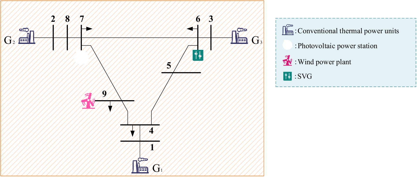
Figure 4: IEEE 9-bus test system topology with locations of renewable energy integration and SVG placement indicated for reactive power optimization studies
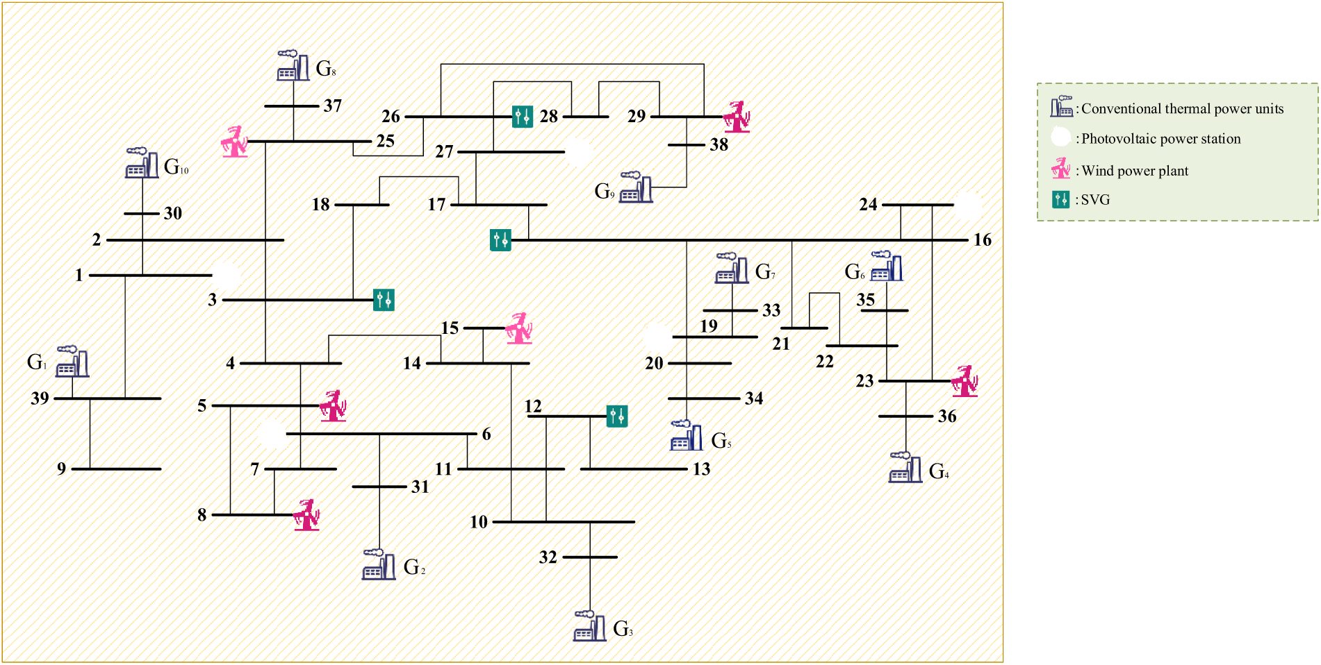
Figure 5: IEEE 39-bus test system topology showing the complex network structure with multiple renewable energy access points and SVG installations for large-scale optimization validation
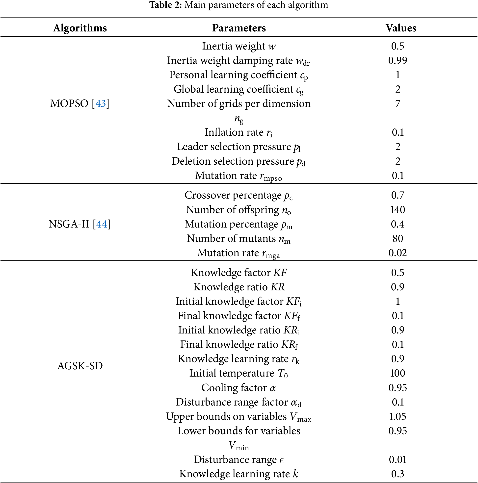
The selection of these specific test systems was deliberate: the IEEE 9-bus system provides a manageable platform for initial algorithm validation, while the more complex IEEE 39-bus system allows for testing scalability and performance under more realistic grid conditions. The non-dominated sorting genetic algorithm-II (NSGA-II) and MOPSO algorithm are selected for benchmark comparison. To ensure fairness in performance evaluation, all algorithms are tested under identical experimental conditions: Each uses a population size of 200, and the maximum number of iterations is set to 200.
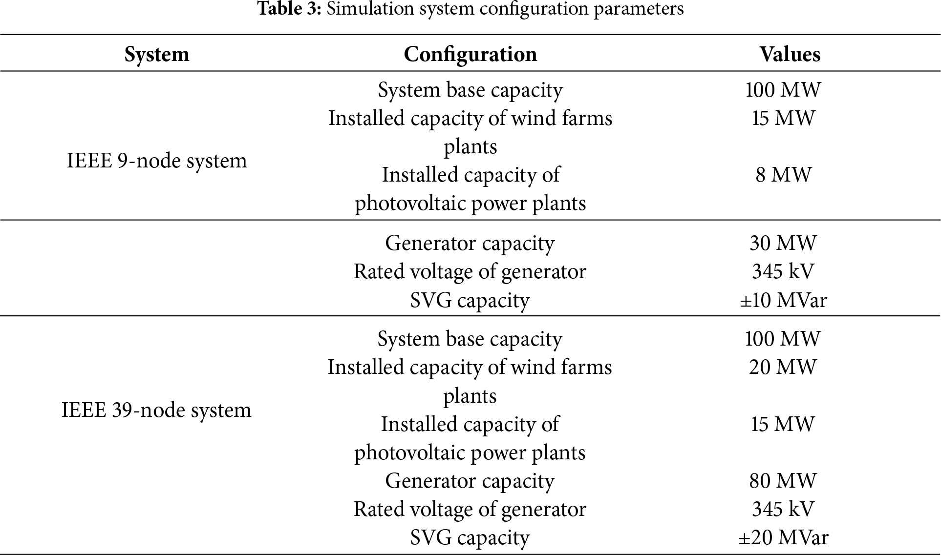
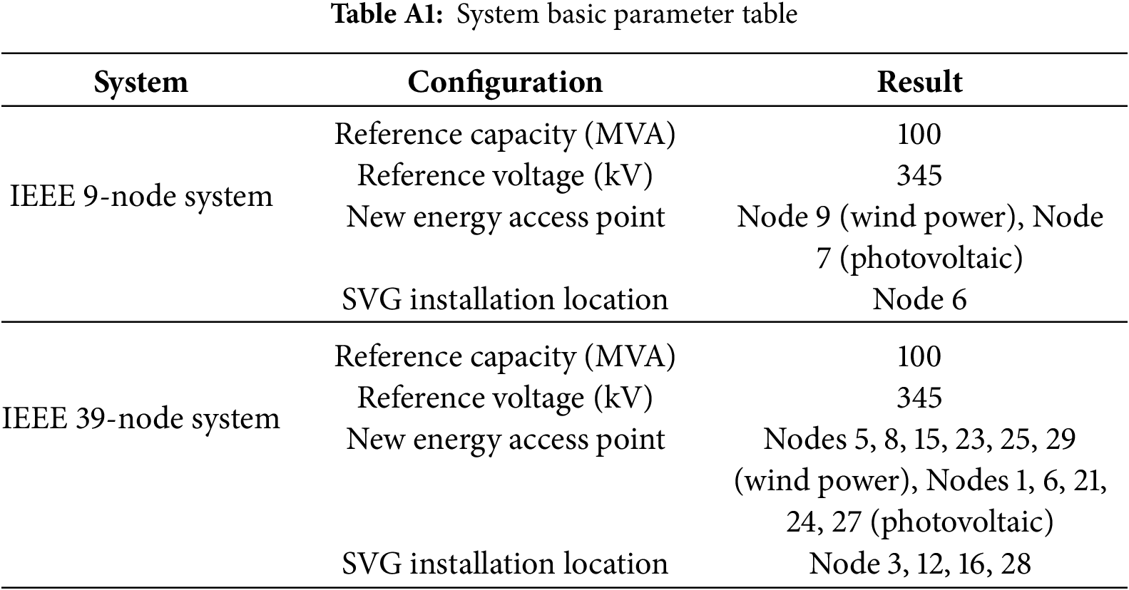
These comparative algorithms were chosen to represent state-of-the-art multi-objective optimization approaches commonly used in power system applications, providing meaningful benchmarks for evaluating our proposed method. The algorithm parameters and the simulation system configuration parameters are shown in Tables 2 and 3, respectively, more detailed system configuration parameters are provided in Tables A1–A4 (Appendix E). The comprehensive parameter sets and repeated testing approach were implemented to ensure robust statistical validation of our results across different system configurations and operating conditions. To ensure the statistical reliability of the experimental conclusions, a repeated testing method is used for performance verification. This study was run on the MATLAB R2023a platform and conducted power flow calculations based on the MATPOWER toolbox. We take the number of iterations as the stopping criterion and use the Newton-Raphson method as the power-flow solver. The hardware environment is an AMD Ryzen 7 5700G processor (with a base frequency of 3.8 GHz and an acceleration frequency of 4.6 GHz). The selection of MATPOWER for power flow calculations was based on its widespread acceptance in academic research and its proven reliability for power system optimization studies, ensuring the reproducibility of our results.
For the simulation system configuration, the reactive power optimization variables of IEEE 9-bus system cover three key dimensions: terminal voltage amplitude adjustment of three synchronous generators on the conventional generation side, discrete configuration parameter optimization of a reactive power optimization device, and two distributed reactive power output controls of new energy power plants. For the larger IEEE 39-bus system, the optimization variable space is significantly expanded, including the voltage regulation of 10 synchronous generators, the discrete configuration parameters of reactive power optimization equipment at 4 locations, and the reactive power output control quantity of 11 new energy stations, forming a more complex multivariate coupling optimization problem.
4.1 Comparative Analysis of Simulation with and without SVG Participation
In power systems, the application of reactive power optimization equipment is important for improving voltage stability and reducing network losses. In this study, the impact of SVG integration is thoroughly analyzed by comparing experimental results with and without SVG deployment across different algorithms and grid model scales. The IEEE 9-bus and IEEE 39-bus systems are selected as test cases, and three algorithms, NSGA-II, MOPSO, and AGSK-SD, are applied for the optimization calculations. The corresponding results are illustrated in Fig. 6. It can be seen that the network power loss and voltage deviations are significantly reduced in the IEEE 9-bus and IEEE 39-bus systems after SVG integration, regardless of whether the NSGA-II algorithm, MOPSO algorithm, or AGSK-SD algorithm. These results confirm that SVG can improve the voltage distribution and enhance the voltage stability of the system while improving energy efficiency and reducing operating costs. The benefits are particularly pronounced in larger and more complex grid models. As shown in Fig. 6, the AGSK-SD algorithm consistently achieves the lowest network loss and voltage deviation across both the IEEE-9 and IEEE-39 systems, regardless of whether SVG is integrated, thereby demonstrating its superior scalability.
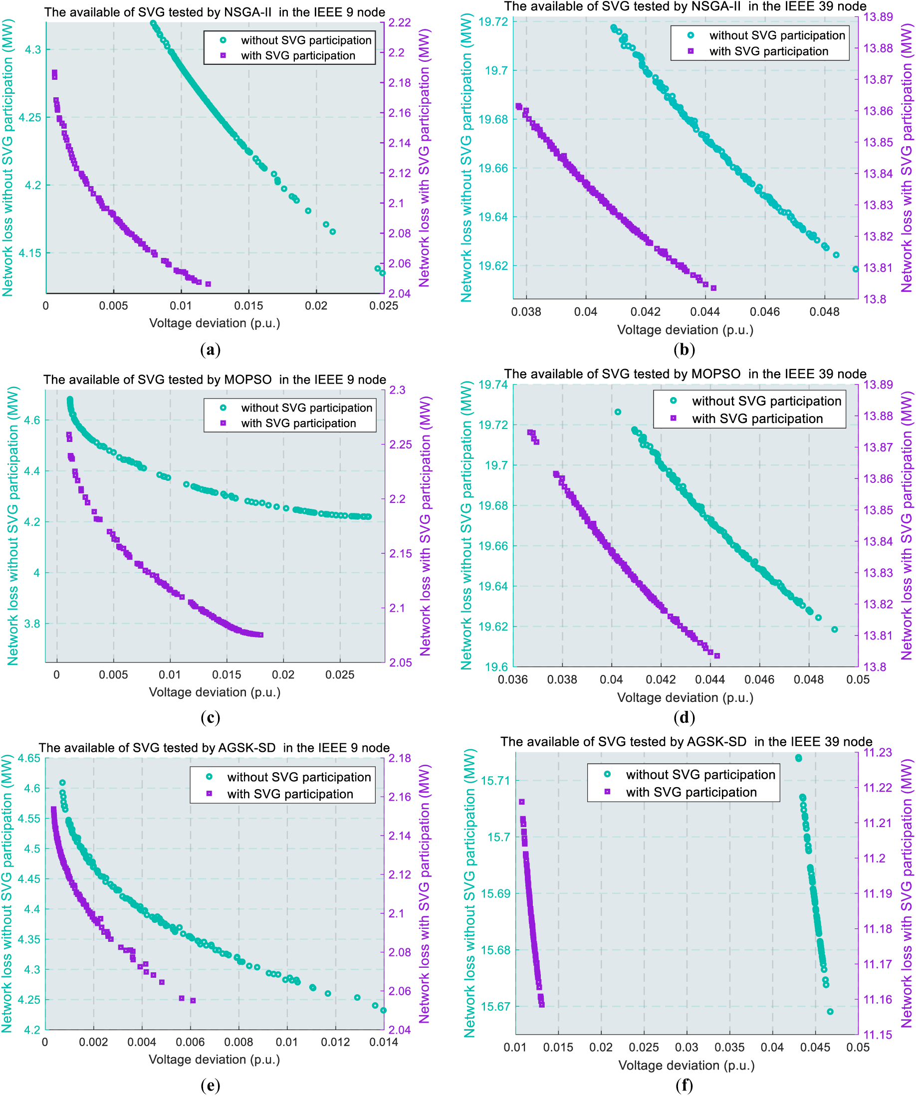
Figure 6: Experimental comparison graphs of reactive power optimization devices applied or not: (a) NSGA-II algorithm comparison graph for IEEE9 nodes; (b) NSGA-II algorithm comparison graph for IEEE39 nodes; (c) MOPSO algorithm comparison graph for IEEE9 nodes; (d) MOPSO algorithm comparison graph for IEEE39 nodes; and (e) AGSK-SD algorithm comparison graph for IEEE9 nodes; (f) AGSK-SD algorithm comparison graph for IEEE39 nodes
Based on these findings, subsequent experiments will continue to introduce SVG to further explore its performance under different grid topologies, operating conditions, and renewable energy penetration rates.
4.2 Comparative Analysis of Reactive Power Optimization Simulations
Based on the topology schematic shown in Figs. 4 and 5, an experimental study on three specific algorithms is carried out. After reactive power optimization, the optimal Pareto solution graphs of various algorithms under each node are shown in Fig. 7. The statistics of the optimization results are shown in Table 4.
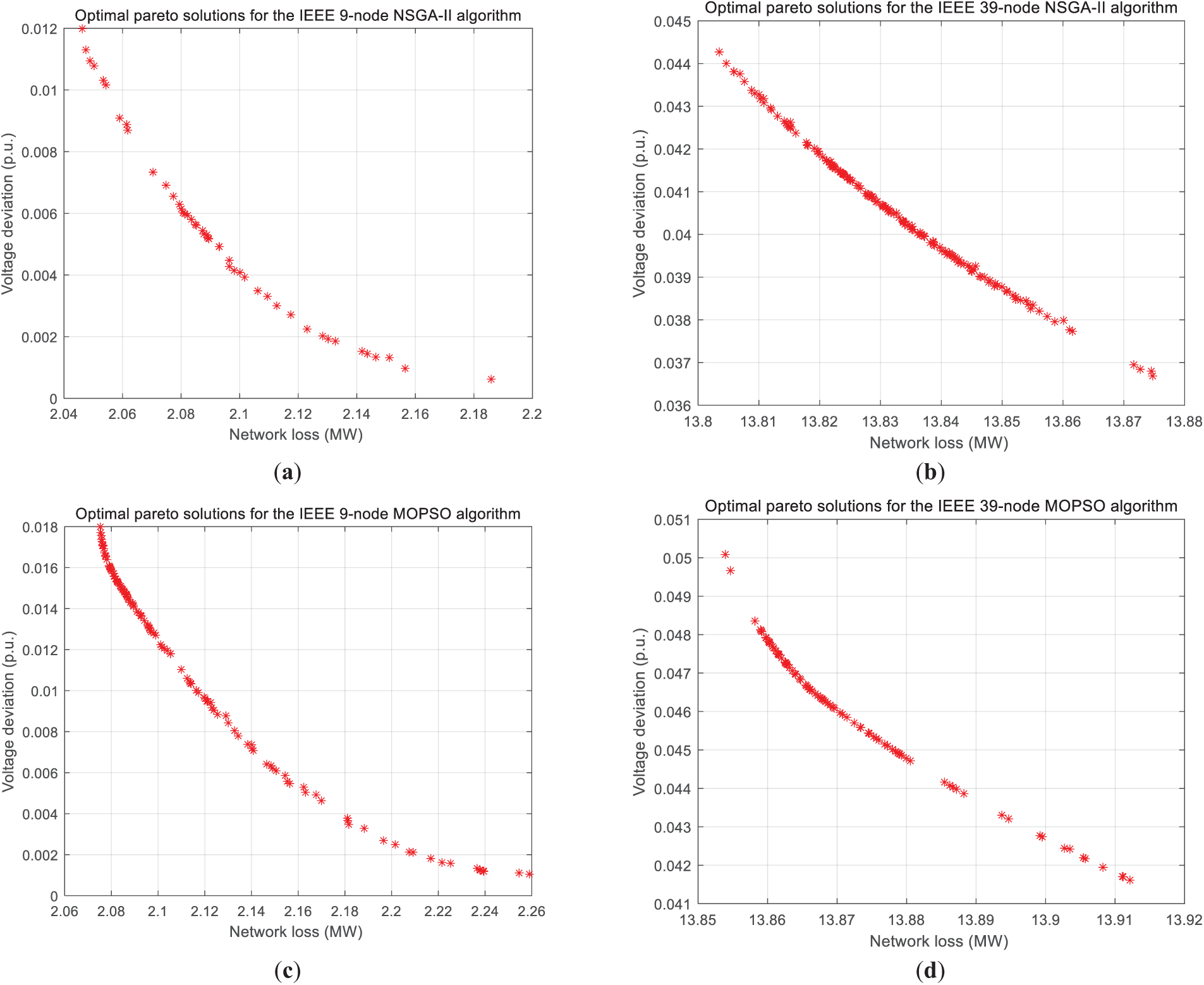
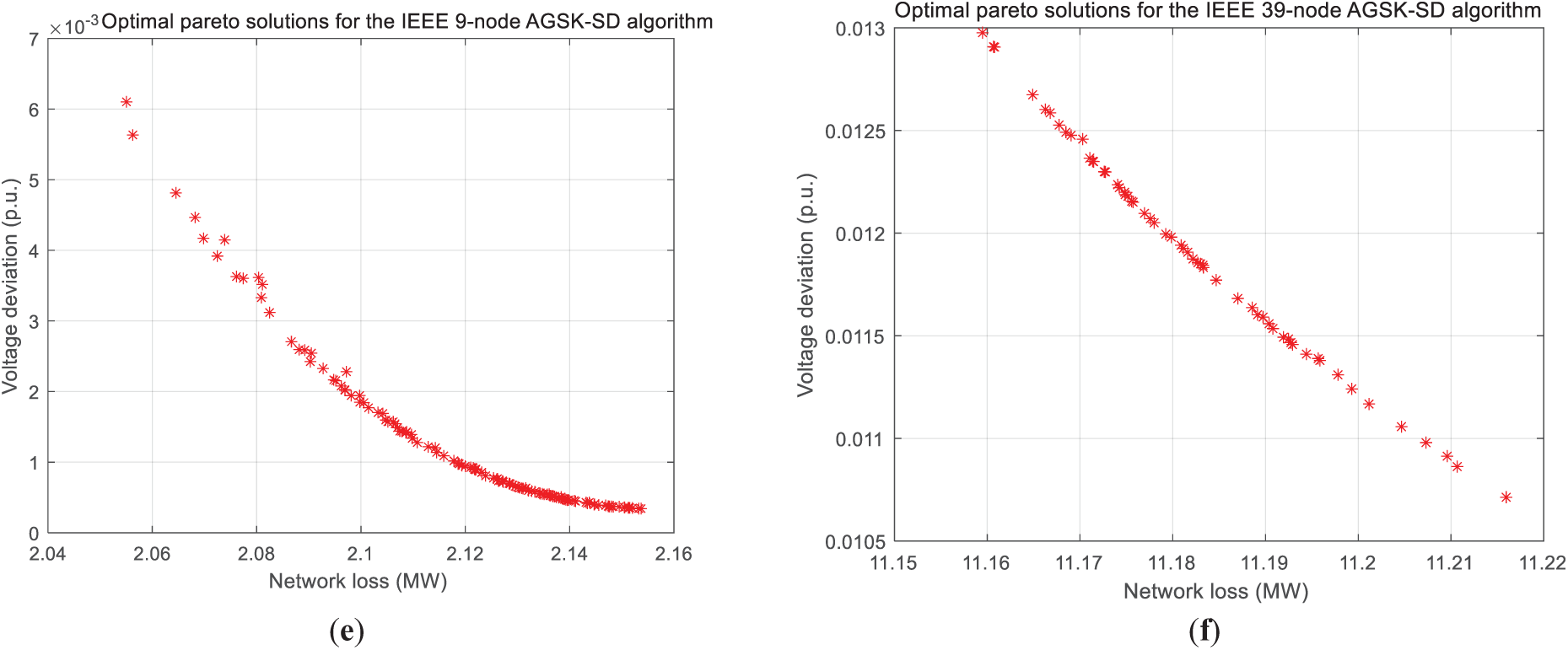
Figure 7: (Optimal pareto solution graph after reactive power optimization: (a) optimization graph of NSGA-II algorithm for IEEE9 nodes; (b) optimization graph of NSGA-II algorithm for IEEE39 nodes; (c) optimization graph of MOPSO algorithm for IEEE9 nodes; (d) optimization graph of MOPSO algorithm for IEEE39 nodes; and (e) optimization graph of AGSK-SD algorithm for IEEE9 nodes; (f) optimization graph of AGSK-SD algorithm for IEEE39 nodes)
By comparing the optimization performance of different algorithms across various-scale grid models, it is clear from Fig. 7 that the non-dominated solution sets generated by different algorithms are uniformly distributed along the two key dimensions, namely, network power loss and voltage deviation. This distribution fully demonstrates the ability of the algorithms to explore trade-offs and identify the balance point between voltage deviation and network loss. Meanwhile, the Pareto trade-off relationship between network power loss and voltage deviation is significant and typical. The Pareto-optimal solution set obtained by AGSK-SD algorithm outperforms the other algorithms in both IEEE 9-bus and IEEE 39-bus grid models in terms of voltage deviation and network loss.
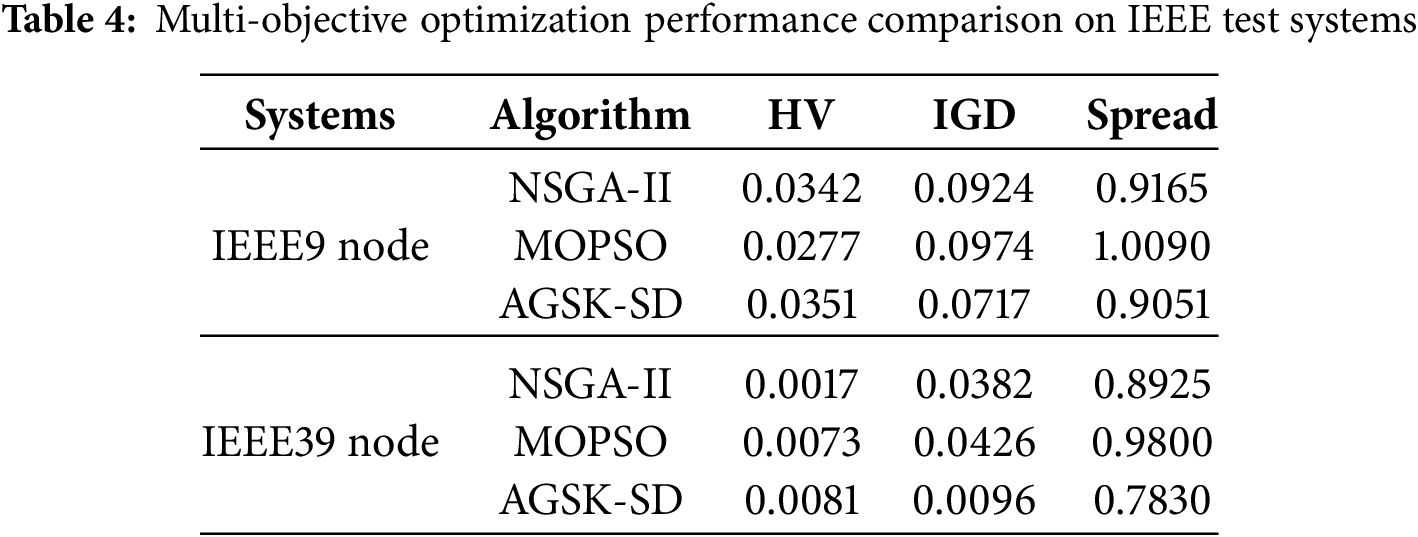
To evaluate and visually present the comprehensive performance of the proposed method in multi-objective optimization, this paper uniformly calculated three recognized indicators, namely hypervolume (HV), inverse generation distance (IGD), and spread, for the Pareto front of IEEE 9-node and 39 node systems. The relevant calculation formulas are shown in Appendix D, the results are listed in the table below.
The table compares the performance of three multi-objective optimization (MOO) algorithms—NSGA-II, MOPSO, and AGSK-SD—in IEEE 9-bus and 39-bus systems, evaluated using three key metrics: HV, IGD, and Spread. The data demonstrates that AGSK-SD consistently outperforms the other algorithms across both system scales. Specifically, AGSK-SD achieves the highest HV values (0.0351 for the 9-bus system and 0.0081 for the 39-bus system) and the lowest IGD values (0.0717 and 0.0096, respectively), indicating superior convergence and proximity to the true Pareto front. Notably, AGSK-SD also maintains the lowest Spread values (0.9051 for the 9-bus system and 0.7830 for the 39-bus system), reflecting better uniformity in solution distribution. In contrast, MOPSO exhibits poorer performance in the 9-bus system with a Spread value of 1.0090, while NSGA-II shows limitations in handling larger systems, as evidenced by its low HV value of only 0.0017 in the 39-bus system. Overall, the table clearly highlights AGSK-SD’s superior and stable performance across different system scales, particularly in terms of solution diversity and convergence, making it the preferred choice for MOO problems in power systems.
These results further validate the superior performance of AGSK-SD algorithm in solving multi-objective optimization problems. In particular, AGSK-SD algorithm is more effective in the more complex IEEE 39-bus system, suggesting that it has a distinct advantage in handling high-dimensional and strongly coupled grid environments. The algorithm achieves a more efficient balance between voltage deviation and network loss, thus enhancing the operational efficiency and reliability of the grid.
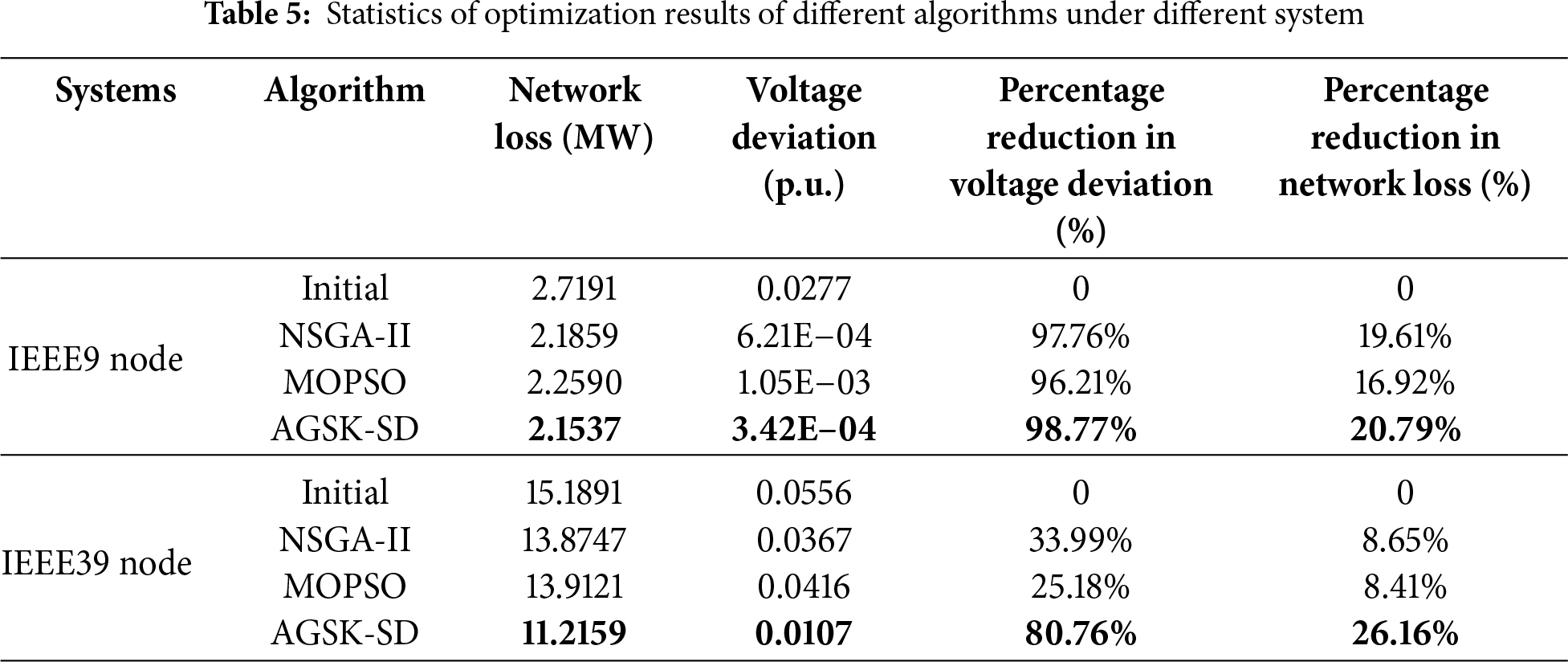
From the data presented in Table 5, it can be seen that although all the algorithms achieve reductions in network loss and voltage deviation, AGSK-SD algorithm consistently demonstrates superior performance across both system configurations. Specifically, after optimization, AGSK-SD algorithm reduces the network loss to 2.1537 and 11.2159 MW in the IEEE 9-bus and IEEE 39-bus systems, respectively, while the voltage deviation is reduced to only 3.42 × 10⁻⁴ and 1.07 × 10⁻² p.u. The corresponding percentage-reduction formulas are given in Appendix C, where the improvements are remarkably high, up to 98.77% and 80.76%, respectively, which are significantly better than that obtained by NSGA-II and MOPSO algorithms. In contrast, NSGA-II algorithm achieves an improvement of 97.76% in IEEE 9-bus system, but only 33.99% in IEEE 39-bus system. This difference shows that NSGA-II algorithm has limited scalability when applied to larger, more complex grid systems. The improvement of MOPSO algorithm in both systems is lower than that of AGSK-SD and NSGA-II algorithms, indicating its weaker global convergence capability. In particular, AGSK-SD algorithm can maintain a voltage quality improvement of over 80% even in the high-dimensional and complex IEEE 39-bus system. This underscores the dual merits of the AGSK-SD algorithm in substantially reducing network losses and concurrently enhancing voltage stability, while further attesting to its remarkable scalability across varying system dimensions, particularly in large-scale optimization environments. Among them, bold values represent the optimal results in each system.
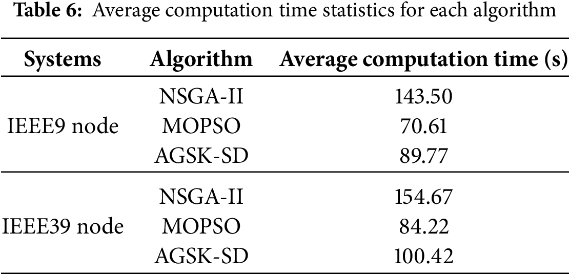
In modern power system dispatch centers, operations are typically divided into different time scales: real-time control (seconds to minutes), rolling one hour advance scheduling (5–15 min), and one-day advance planning (hours). The observed running time from Table 6 is approximately 100 s (less than 2 min), making the AGSK-SD algorithm advantageous for near real time and rolling horizon optimization applications. This time range is acceptable for adjusting reactive power settings in response to slowly changing conditions, such as different renewable energy generation forecasts and load patterns, which are typically updated every 5 to 15 min.
For integration into a true real-time control framework (e.g., sub-minute cycles), further acceleration would be desirable. Several strategies could be explored to achieve this:
(1) Parallelization: The AGSK-SD algorithm is inherently parallelizable. The evaluation of individual agents in the population can be distributed across multiple CPU cores or compute nodes, potentially reducing the computation time nearly linearly with the number of available processors.
(2) GPU Acceleration: The matrix and vector operations central to the heuristic search process could be efficiently offloaded to a Graphics Processing Unit (GPU), leveraging its massive parallelism to achieve significant speedups, likely reducing runtimes to within tens of seconds.
(3) Hybrid Implementation: A practical implementation could combine a fast, simplified model for frequent real-time corrections with the detailed AGSK-SD optimization triggered at a slower interval (e.g., every 15 min) to provide a new optimal baseline, ensuring both accuracy and responsiveness.
All the calculations are done in Matlab 2023a platform, and the trend calculation is done by MATPOWER built-in solver. The average computation time shown in the above table indicates that all the algorithms meet the real-time scheduling requirements. Although AGSK-SD does not take the shortest time, it brings the largest reduction of voltage deviation and network loss, and has the most compact box-and-line diagram under 50 independent runs, which is significantly better than NSGA-II and MOPSO in terms of robustness, and has the best overall performance.
4.3 Algorithm Stability Analysis
To further verify the effectiveness of AGSK-SD algorithm in reactive power optimization, this study conducts 50 independent runs for each algorithm. The results are then comprehensively analyzed to evaluate and compare their convergence stability and global search capability. Under the premise of minimizing grid loss and voltage deviation as the optimization objectives, Fig. 8 shows the statistical results of grid loss and voltage deviation for different algorithms, visualized in the form of box-and-whisker plots.
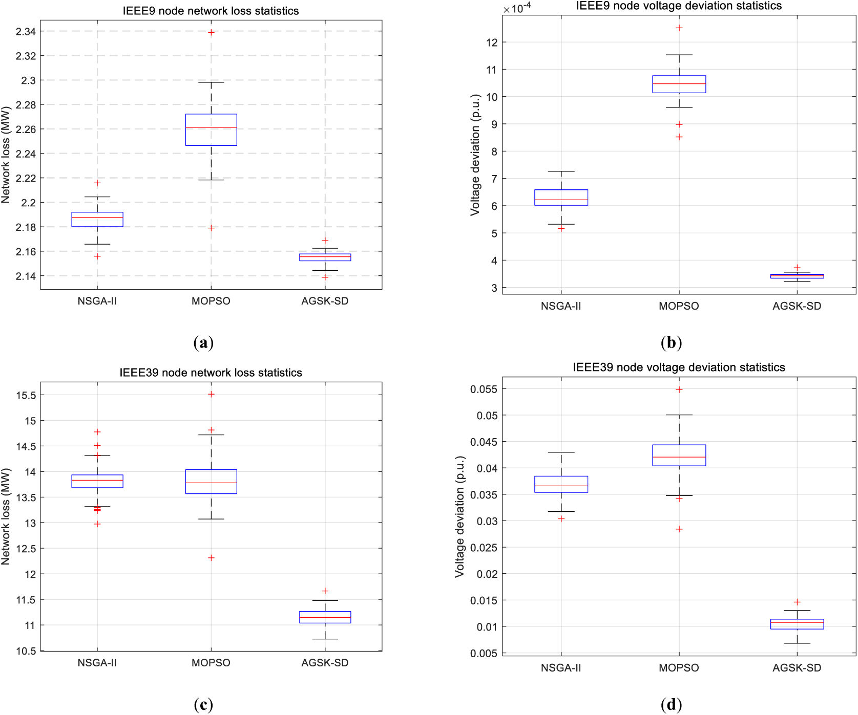
Figure 8: Box-and-whisker plots of statistical results for 50 runs of different algorithms: (a) IEEE9 node network loss; (b) IEEE9 node voltage deviation; (c) IEEE39 node network loss; (d) IEEE39 node voltage deviation
The data presented in Fig. 8 shows that AGSK-SD algorithm exhibits superior stability and performance in terms of network loss control and voltage deviation adjustment in IEEE 9-bus system. The corresponding box-and-whisker plot distributions are relatively concentrated and maintained at low levels, which strongly indicates that the algorithm’s effectiveness in minimizing both network losses and voltage deviations. When applied to the more complex IEEE 39-bus system, AGSK-SD algorithm also shows outstanding advantages in the statistics of network loss and voltage deviation. The statistical results are not only significantly better than the other two algorithms, but also exhibit a more compact data distribution. These outcomes further substantiate the outstanding effectiveness and algorithmic stability of the AGSK-SD algorithm in reactive-power optimization of complex power systems, while reiterating its remarkable scalability across varying scales.
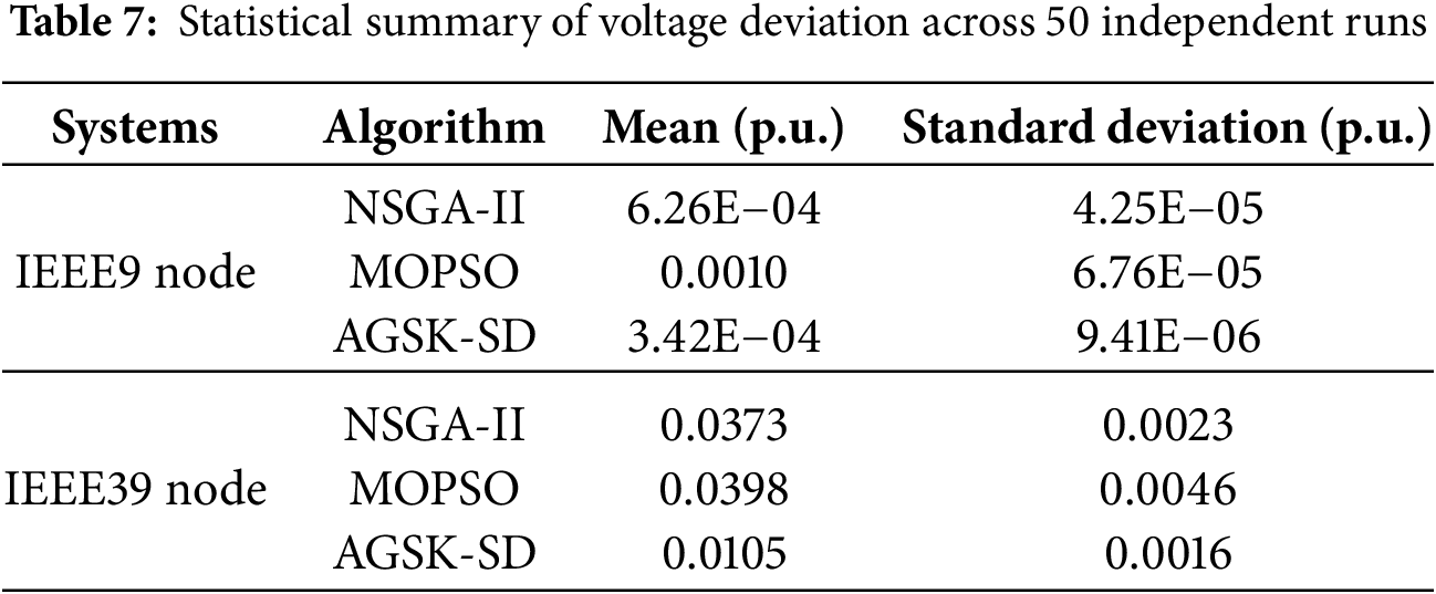
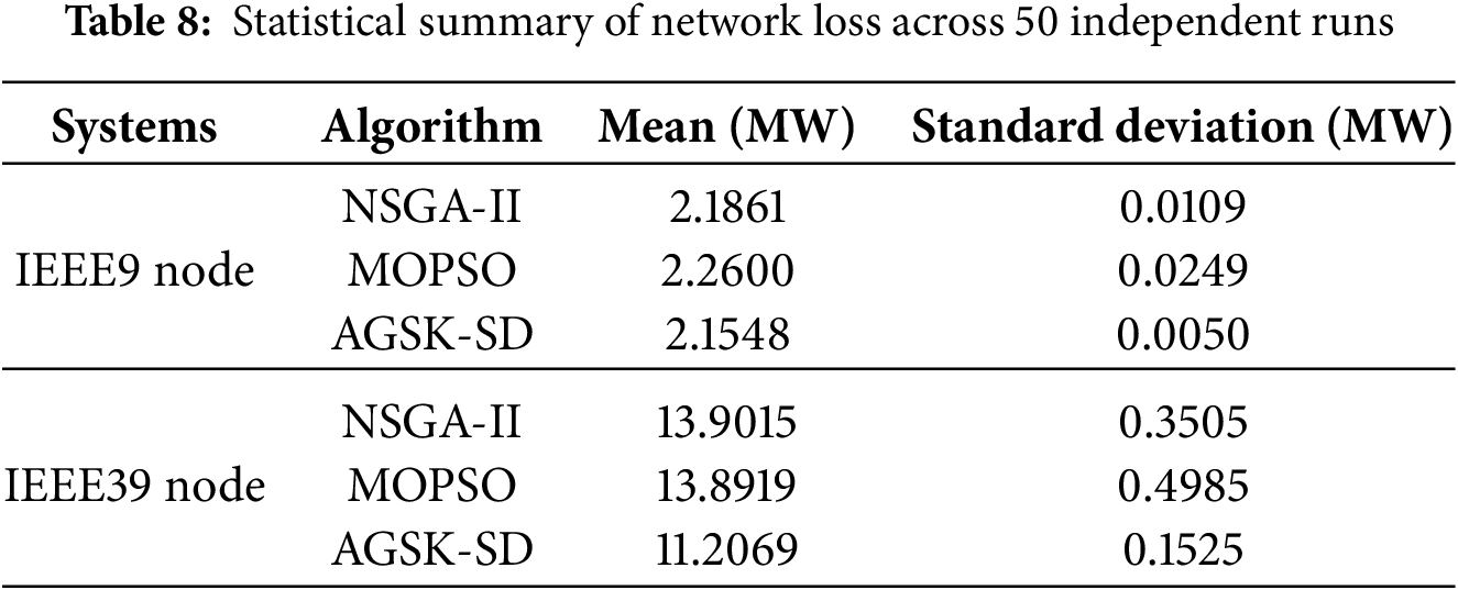
Based on the statistical data of 50 independent runs shown in Fig. 8, we conducted a comprehensive statistical analysis to rigorously evaluate the performance of the algorithm. The results are shown in Tables 7 and 8 below. AGSK-SD showed statistically significant improvements in all measurement indicators compared to NSGA-II and MOPSO. For voltage deviation, AGSK-SD achieved excellent performance, with an average ± standard deviation of 3.42E−04 ± 9.41E−06 p.u. (IEEE 9-node) and 0.0105 ± 0.0016 p.u. (IEEE 39 node), respectively, which were reduced by 45.4% and 71.8% compared to NSGA-II. Similarly, for network loss, AGSK-SD maintained lower average ± SD values of 2.1548 ± 0.0050 MW (IEEE 9-node) and 11.2069 ± 0.1525 MW (IEEE 39 node), which were 1.43% and 19.4% higher than NSGA-II, respectively. These statistically validated results, combined with narrow standard deviations, demonstrate the excellent optimization capability and robust stability of the proposed AGSK-SD algorithm at different system scales.
4.4 Comparison and Analysis of Data at Each Node
Figs. 9 and 10 show the network losses and voltage deviations corresponding to each node when comparing the three algorithms with the initial state.

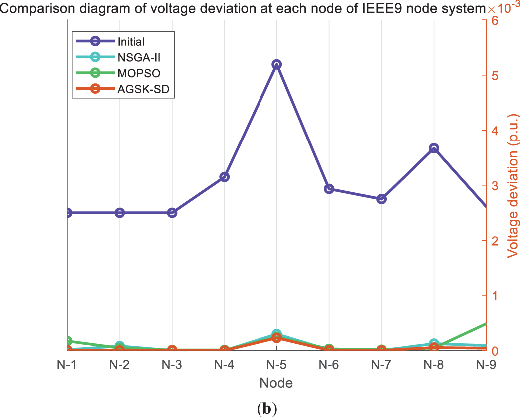
Figure 9: IEEE9 node system situation map for each node: (a) network loss comparison chart; (b) voltage deviation comparison chart
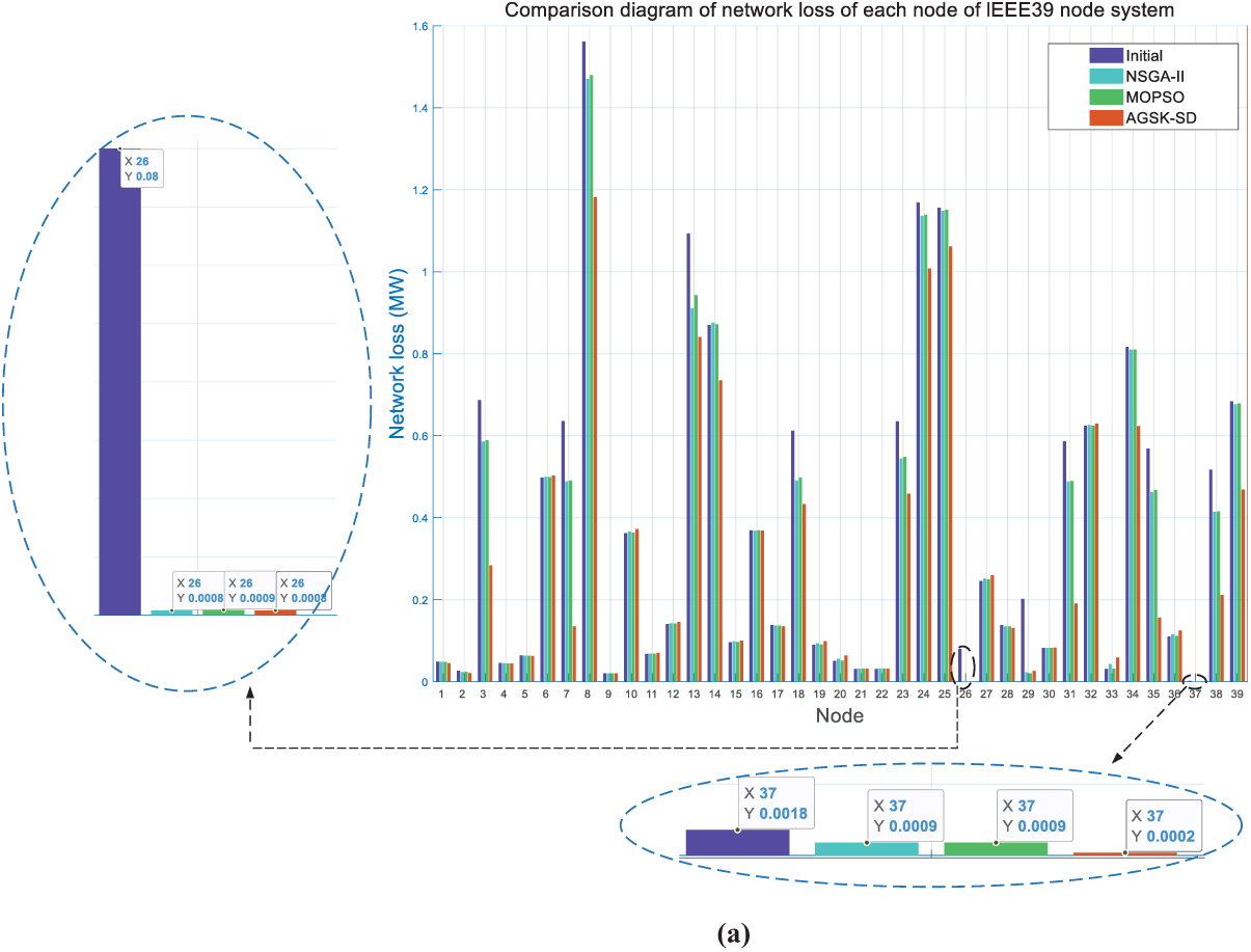
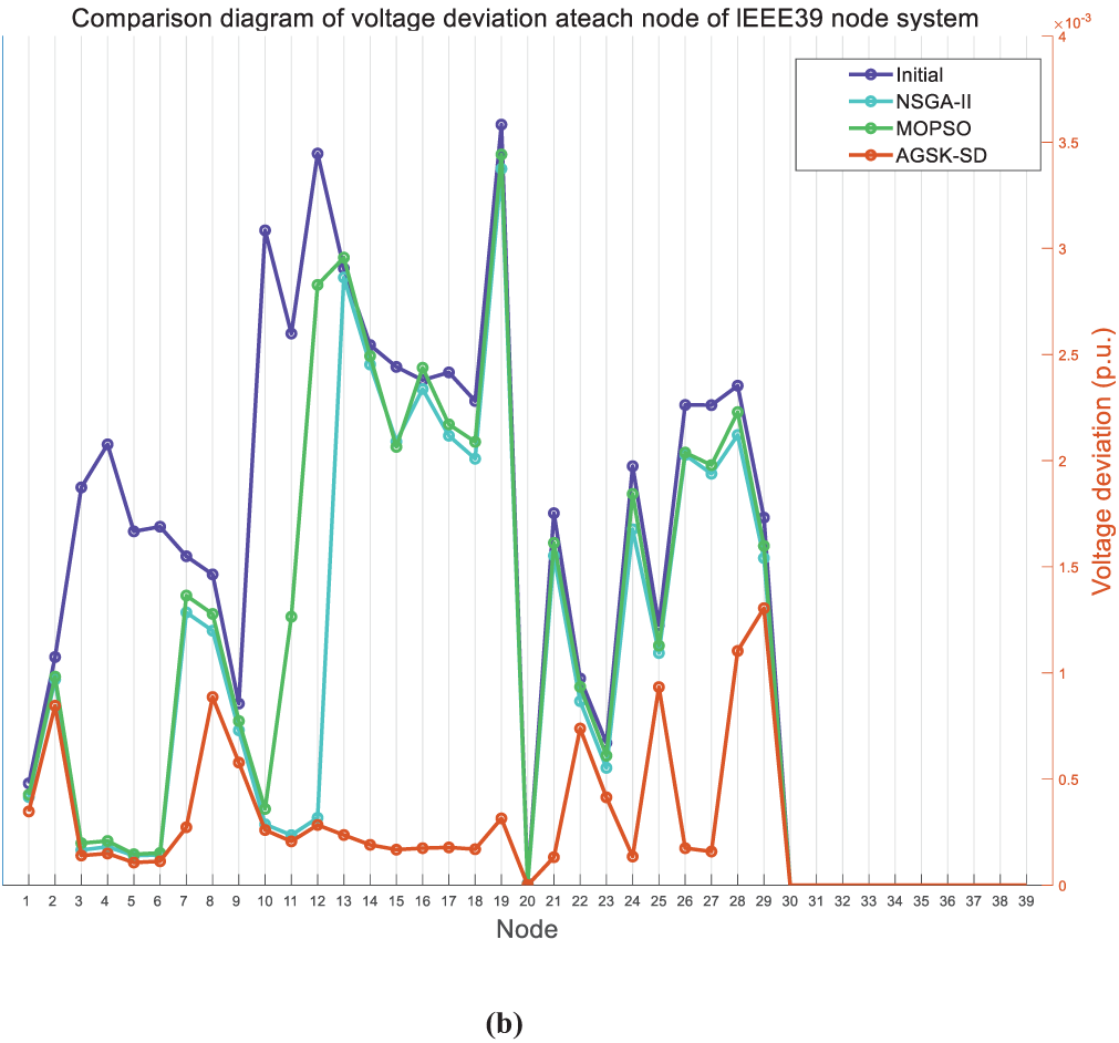
Figure 10: IEEE39 node system situation map for each node: (a) network loss comparison chart; (b) voltage deviation comparison chart
From the results presented in Figs. 9 and 10, it can be seen that in both systems under study, not all nodes exhibit a reduction in network losses after optimization. In some cases, the network loss at certain nodes remains unchanged or even increases compared to the initial state. However, at the system level, the total network loss after optimization is reduced compared with the initial state. At the same time, the voltage deviation of individual nodes, as well as the overall system voltage deviation, consistently show a decreasing trend regardless of the optimization algorithm applied. Further comparison of the optimization results in the two systems reveals that AGSK-SD algorithm achieves the best performance, especially in IEEE 39-bus system, where the algorithm can minimize the voltage deviation of the system.
4.5 Analysis of the Impact of Changes in the Proportion of New Energy Access on Reactive Power Optimization
To investigate the effects of different renewable energy penetration levels on the reactive power optimization of the grid with integrated wind and PV energy, and to ensure the comprehensiveness and accuracy of the evaluation, this section selects IEEE 9-bus system and IEEE 39-bus system as research platforms, and statistically analyzes the optimization results of AGSK-SD algorithm under varying penetration levels of renewable energy The corresponding results are presented in Fig. 11. When the proportion of renewable energy in the grid is increasing, its inherent intermittency and randomness, along with the potential reverse power flow, have a significant impact on the stable operation of the grid system. Specifically, line loss and voltage deviation show a synchronized and continuously increasing trend. The reason is that with the higher renewable penetration rate, the volatility of its output increases. In addition, reverse power flows increase the line current, disrupting the reactive power balance and ultimately causing simultaneous increases in line losses and voltage deviations.
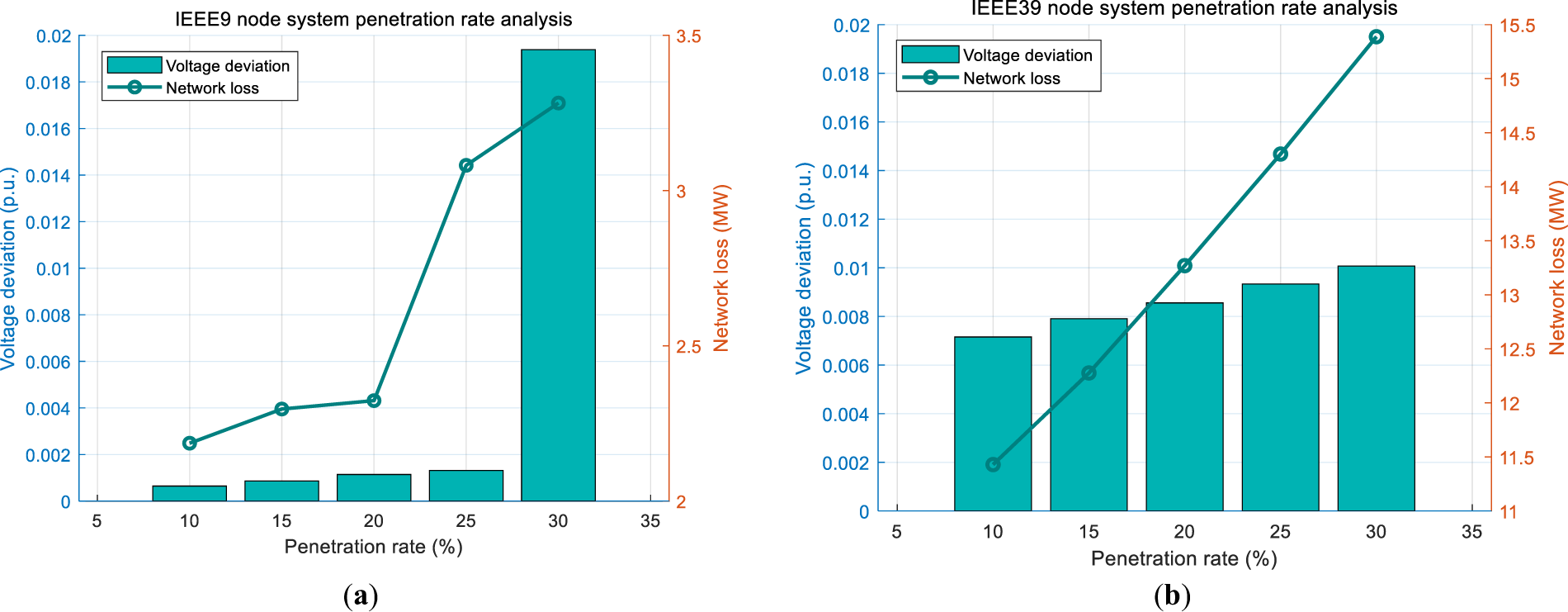
Figure 11: Analysis of different renewable energy penetration levels: (a) IEEE 9-node system; (b) IEEE 39-node system
To address the voltage fluctuations and increased network losses caused by the integration of wind and solar energy, this work constructs an integrated multi-objective optimization model that simultaneously incorporates the real-time reactive power margins of wind turbines, PV inverters, and SVGs. Further, a AGSK-SD algorithm is developed, which couples the adaptive knowledge factor/ratio, simulated annealing fine search, and diversity perturbation in the GSK framework. Experimental results confirm the following findings:
(1) This work incorporates the real-time reactive power adjustable potentials of wind turbines, PV units, and SVGs into a unified optimization model. Applying this model resulted in voltage deviation reductions of 98.77% and 80.76% in the IEEE 9-bus and 39-bus systems, respectively. These results surpass the performance of both NSGA-II and MOPSO algorithms.
(2) Within the GSK framework, we introduce an adaptive control mechanism that dynamically tunes the KF and KR. In the IEEE 39-bus system, the proposed AGSK-SD algorithm surpasses NSGA-II by cutting network losses by 17.75% and shrinking voltage deviation by 40.77%. Crucially, it refines late-stage local search accuracy without enlarging computational complexity, thereby offering a practical route for high-dimensional power-grid fine-tuning.
(3) The AGSK-SD algorithm embeds a simulated-annealing-based fine-grained local searcher and a periodic diversity-perturbation operator into the GSK framework. This implementation creates an annealing-probability-driven mechanism that effectively escapes local optima. It also cyclically enlarges the exploration domain to strengthen the global search. Their synergy yields a Pareto front whose uniformity and extent of coverage markedly exceed those delivered by NSGA-II and MOPSO. Statistical verification across fifty independent executions reveals markedly tighter boxplots, underscoring the algorithm’s superior robustness, stability, and consistency, together with consistently lower terminal objective values.
The proposed transmission level reactive power optimization framework and AGSK-SD algorithm demonstrate excellent performance in the power grid, outperforming NSGA-II and MOPSO in voltage deviation control and loss reduction in batch renewable energy integration scenarios. Optimised set-points can be streamed to wind converters, PV inverters and SVGs within seconds, exploiting existing assets to boost renewable absorption and defer line upgrades while meeting European RfG. Recommended deployment is a lightweight AGSK-SD module in regional control centres, prioritising firmware upgrades at high-penetration nodes, and mapping results to day-ahead reactive-power bids to cut reserve costs. steady-state assumptions, no short-circuit, dynamic reserve or delay, and 9/39-bus scope—will be addressed via dynamic simulation, probabilistic uncertainty and communication latency before provincial-scale hardware-in-the-loop validation. AGSK-SD can be fused with deep-learning-based renewable forecasts for millisecond “forecast–optimize–dispatch” loops, inherently suits hybrid AC/DC grids, and aligns with emerging plug-and-play, cloud-edge, and digital-twin frameworks. yet scaling to ultra-large networks still faces surging computation, communication latency and high-precision meteorological data dependence.
Despite its promising results, this study has limitations that outline directions for future work. The research relies on steady-state assumptions. It does not capture dynamic behaviors or the uncertainty inherent in renewable generation and load demand. These omissions may impact the robustness of the solutions in real operations. Additionally, validation was conducted on medium-scale test systems (IEEE 9-bus and 39-bus), and performance on larger real-world networks remains to be verified. Future efforts will focus on integrating uncertainty modeling through stochastic programming, extending the framework to dynamic optimization, applying the method to large-scale systems with accelerated computing, and validating results via hardware-in-the-loop testing to bridge the gap between theoretical development and practical industry application.
Acknowledgement: Special appreciation is extended to the engineers and researchers from Yunnan Power Grid Co., Ltd. for their technical support and data assistance during the development of this study.
Funding Statement: This work was supported by Yunnan Power Grid Co., Ltd. Science and Technology Project: Research and application of key technologies for graphical-based power grid accident reconstruction and simulation (YNKJXM20240333).
Author Contributions: The authors confirm contribution to the paper as follows: Conceptualization, writing—original draft and writing—review & editing: Xuan Ruan; Methodology: Han Yan; Validation: Donglin Hu; Formal analysis: Min Zhang; Investigation: Ying Li.; Data processing: Di Hai; Funding acquisition and writing—original draft: Bo Yang. All authors reviewed the results and approved the final version of the manuscript.
Availability of Data and Materials: The authors confirm that the data supporting the findings of this study are available within the article.
Ethics Approval: Not applicable.
Conflicts of Interest: The authors declare no conflicts of interest to report regarding the present study.
Nomenclature
| Abbreviations | |
| AGSK-SD | Adaptive gain shared knowledge with simulated annealing and diversity maintenance |
| EV | Electric vehicle |
| GIPA | Genetic interior-point algorithm |
| GSK | Gain shared knowledge |
| HA | Heuristic algorithm |
| KF | Knowledge factor |
| KR | Knowledge ratio |
| MINLP | Mixed integer nonlinear programming |
| MOO | Multi-objective optimization |
| MOPSO | Multi-objective particle swarm optimization |
| MICP | Mixed integer convex programming |
| MPPT | Maximum power point tracking |
| NSGA-II | Non-dominated sorting genetic algorithm II |
| ORPD | Optimal reactive power distribution |
| PSO | Particle swarm optimization |
| PV | Photovoltaic |
| REGC | Renewable energy grid-connection |
| RMS | Root-mean-square |
| SOO | Single-objective optimization |
| SVG | Static var generator |
| SA | Simulated annealing |
| Variables | |
| Power conversion coefficient reflecting the temperature characteristics of PV module | |
| Rated power of PV plant | |
| Light intensity received by PV array | |
| Real-time air temperature of the environment where PV plant | |
| Reference value of the air temperature used for power correction | |
| Rated capacity parameter of PV inverter | |
| Wind speed at the current moment | |
| Rated wind speed of the wind turbine | |
| Cooling factor | |
| Random perturbation vector | |
| Stator inductance | |
| Excitation inductance | |
| Slew rate | |
| Synchronous rotational angular velocity | |
| Rotor rotational angular velocity | |
| Value of the stator voltage | |
| System voltage phasor | |
| SVG voltage phasor | |
| Voltage phasor across the reactor | |
| Current phasor flowing through the reactor | |
| Total active power loss of the entire power network | |
| Sum of the deviations from the nominal value of the voltage at each node of the grid | |
| Voltage amplitude of node i | |
| Voltage amplitude of node j | |
| Difference in the phase angle between the two nodes | |
| Branch conductance between node i and node j | |
| Collection of all the nodes in the power system | |
| Set of all transmission branches | |
| Active power output from the generator at node i | |
| Reactive power output from the generator at node i | |
| Active load demand carried by node i | |
| Reactive load demand carried by node i | |
| Collection of transformer taps | |
| Set of all nodes in the power system excluding the balancing node | |
| Active power output from the generator at the balancing node | |
| Set of all generators in the power system | |
| Collection of reactive power optimization devices | |
| Apparent power of line l | |
| Set of all lines in the system | |
| Knowledge learning rate | |
| Knowledge factor parameter | |
| Initial temperature | |
| Current temperature | |
Appendix A Reactive Power Regulation Boundary Constraints
The reactive power regulation range on the stator side is mainly influenced by the maximum current constraints that can be carried on the stator and rotor sides, as follows [33]:
where
From another point of view, the reactive power regulation range of the grid-side converter is primarily determined by its own capacity limitations, as follows [33]:
where
Appendix B SVG Modelling Details
Fig. A1 reproduces the three-phase voltage-source SVG bridge used in this study [45].
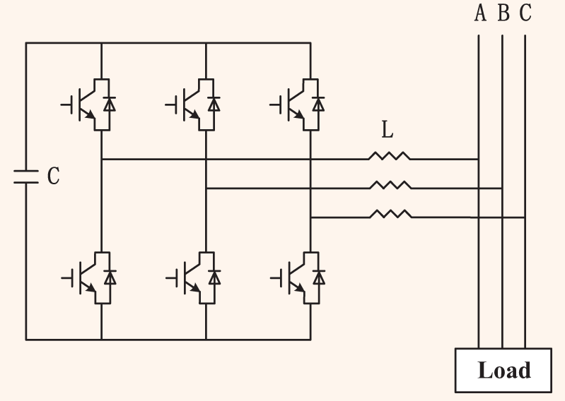
Figure A1: Bridge circuit for voltage type SVG
By adjusting the magnitude and phase of the AC-side voltage generated by its bridge converter, the SVG can rapidly inject or absorb reactive power with high precision. Its control is highly flexible and its response is fast enough to counteract sudden load changes. Compared with other compensating devices, the SVG offers clear technical advantages. Fig. A2 shows the lossless equivalent circuit [45,46]:
Based on the fundamental principles of circuit theory, the reactor current can be expressed as [45]:
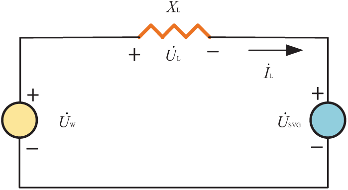
Figure A2: Schematic representation of the equivalent circuit for SVG
The complex power transferred to SVG system is described by:
The SVG is designed to operate without consuming active power. Moreover, the phase disparity between the grid-side voltage and the SVG AC-side voltage is assumed to be zero. Consequently, based on Eq. (A6), the reactive power absorbed by SVG can be derived as follows [46]:
where
By adjusting the magnitude and phase angle of SVG’s output voltage
Appendix C Percentage-Reduction Calculation
To intuitively quantify the comprehensive benefits of reactive-power optimization in terms of voltage-profile improvement and network-loss reduction, this paper introduces a unified percentage-decrease metric for the two key indices—voltage deviation and total power loss—as defined in the following equation.
where,
Appendix D Calculation Instructions for HV, IGD, and Spread
1. Hypervolume (HV)
HV is the spatial volume enclosed by the Pareto front and reference point. Let the approximate frontier and reference point be:
HV is the Lebesgue measure of the region dominated by at least one solution in
where
2. Inverse Generative Distance (IGD)
IGD is the average distance from the true Pareto front to the solution set obtained by the algorithm. Let the real Pareto front uniform sampling point set be:
where
3. Distribution Indicator Spread
Spread is the degree of uniformity of the distribution of the solution set in the target space. Let the true frontier endpoint and approximate frontier endpoint be:
From the above equation, it can be concluded that:
where
Appendix E Detailed System Configuration Parameters
The detailed data parameters of the extended IEEE 9-node and 39 node testing systems are supplemented as follows:
References
1. He B, Yang B, Han Y, Zhou Y, Hu Y, Shu H, et al. Optimal EVCS planning via spatial-temporal distribution of charging demand forecasting and traffic-grid coupling. Energy. 2024;313(6):133885. doi:10.1016/j.energy.2024.133885. [Google Scholar] [CrossRef]
2. Zhu J, Miao Y, Dong H, Li S, Chen Z, Zhang D. Short-term residential load forecasting based on K-shape clustering and domain adversarial transfer network. J Mod Power Syst Clean Energy. 2024;12(4):1239–49. [Google Scholar]
3. Hu Y, Yang B, Wu P, Wang X, Li J, Huang Y, et al. Optimal planning of electric-heating integrated energy system in low-carbon park with energy storage system. J Energy Storage. 2024;99(1):113327. doi:10.1016/j.est.2024.113327. [Google Scholar] [CrossRef]
4. Liang Y, Lin S, Lai X, Liu M, Zhang B. Coordinated planning for multiple inner networks of offshore wind farms and onshore transmission expansion. Prot Control Mod Power Syst. 2025;10(3):35–54. doi:10.23919/PCMP.2024.000078. [Google Scholar] [CrossRef]
5. Yang B, Qian YC. A review on the state-of-health estimation for lithium-ion batteries. J Kunming Univ Sci Technol Nat Sci. 2024;49(3):147–65. doi:10.16112/j.cnki.53-1223/n.2024.05.451. [Google Scholar] [CrossRef]
6. Wang Y, Liu Y, Liu C, Cai G, Zhang X, Liu K, et al. Bipolar direct AC/AC conversion-based dual-bus parallel supply system and its flexible regulation characteristics. Prot Control Mod Power Syst. 2025;10(3):114–24. doi:10.23919/PCMP.2024.000072. [Google Scholar] [CrossRef]
7. Li J, Yang B, Huang J, Guo Z, Wang J, Zhang R, et al. Optimal planning of electricity–hydrogen hybrid energy storage system considering demand response in active distribution network. Energy. 2023;273(1):127142. doi:10.1016/j.energy.2023.127142. [Google Scholar] [CrossRef]
8. Yang B, Zhou Y, Yan Y, Su S, Li J, Yao W, et al. A critical and comprehensive handbook for game theory applications on new power systems: structure, methodology, and challenges. Prot Control Mod Power Syst. 2025;10(5):1–27. doi:10.23919/PCMP.2024.000297. [Google Scholar] [CrossRef]
9. Han S, He M, Zhao Z, Chen D, Xu B, Jurasz J, et al. Overcoming the uncertainty and volatility of wind power: day-ahead scheduling of hydro-wind hybrid power generation system by coordinating power regulation and frequency response flexibility. Appl Energy. 2023;333(5):120555. doi:10.1016/j.apenergy.2022.120555. [Google Scholar] [CrossRef]
10. Luo X, Zhang D. An adaptive deep learning framework for day-ahead forecasting of photovoltaic power generation. Sustain Energy Technol Assess. 2022;52(6):102326. doi:10.1016/j.seta.2022.102326. [Google Scholar] [CrossRef]
11. Che EE, Roland Abeng K, Iweh CD, Tsekouras GJ, Fopah-Lele A. The impact of integrating variable renewable energy sources into grid-connected power systems: challenges, mitigation strategies, and prospects. Energies. 2025;18(3):689. doi:10.3390/en18030689. [Google Scholar] [CrossRef]
12. Dimnik J, Topić Božič J, Čikić A, Muhič S. Impacts of high PV penetration on Slovenia’s electricity grid: energy modeling and life cycle assessment. Energies. 2024;17(13):3170. doi:10.3390/en17133170. [Google Scholar] [CrossRef]
13. Iung AM, Cyrino Oliveira FL, Marcato ALM. A review on modeling variable renewable energy: complementarity and spatial-temporal dependence. Energies. 2023;16(3):1013. doi:10.3390/en16031013. [Google Scholar] [CrossRef]
14. Purlu M, Turkay BE. Optimal allocation of renewable distributed generations using heuristic methods to minimize annual energy losses and voltage deviation index. IEEE Access. 2022;10(1):21455–74. doi:10.1109/ACCESS.2022.3153042. [Google Scholar] [CrossRef]
15. Xiong M, Yang X, Zhang Y, Wu H, Lin Y, Wang G. Reactive power optimization in active distribution systems with soft open points based on deep reinforcement learning. Int J Electr Power Energy Syst. 2024;155(2):109601. doi:10.1016/j.ijepes.2023.109601. [Google Scholar] [CrossRef]
16. Ni S, Cui CG, Yang N, Chen H, Xi PF, Li ZK. Multi-time-scale online optimization for reactive power of distribution network based on deep reinforcement learning. Autom Electr Power Syst. 2021;45(10):77–85. doi:10.7500/AEPS20200830003. [Google Scholar] [CrossRef]
17. Huang DW, Wang XQ, Yu N, Chen HH. Hybrid timescale voltage/var control in distribution network considering PV power uncertainty. Trans China Electrotech Soc. 2022;37(17):4377–89. doi:10.19595/j.cnki.1000-6753.tces.211188. [Google Scholar] [CrossRef]
18. Mas’ud AA, Seidu I, Salisu S, Musa U, AlGarni HZ, Bajaj M, et al. Wind energy assessment and hybrid micro-grid optimization for selected regions of Saudi Arabia. Sci Rep. 2025;15(1):1376. doi:10.1038/s41598-025-85616-9. [Google Scholar] [PubMed] [CrossRef]
19. Gu Z, Li B, Zhang G, Li B. Optimizing photovoltaic integration in grid management via a deep learning-based scenario analysis. Sci Rep. 2025;15(1):14851. doi:10.1038/s41598-025-98724-3. [Google Scholar] [PubMed] [CrossRef]
20. Mahmoudi SM, Maleki A, Rezaei Ochbelagh D. Multi-objective optimization of hybrid energy systems using gravitational search algorithm. Sci Rep. 2025;15(1):2550. doi:10.1038/s41598-025-86476-z. [Google Scholar] [PubMed] [CrossRef]
21. Li Z, Xiong J. Reactive power optimization in distribution networks of new power systems based on multi-objective particle swarm optimization. Energies. 2024;17(10):2316. doi:10.3390/en17102316. [Google Scholar] [CrossRef]
22. Farhat M, Kamel S, Abdelaziz AY. Modified Tasmanian devil optimization for solving single and multi-objective optimal power flow in conventional and advanced power systems. Clust Comput. 2024;28(2):105. doi:10.1007/s10586-024-04790-z. [Google Scholar] [CrossRef]
23. Álvarez O, Carrión D, Jaramillo M. Optimal reactive power dispatch planning considering voltage deviation minimization in power systems. Energies. 2025;18(11):2982. doi:10.3390/en18112982. [Google Scholar] [CrossRef]
24. Xu B, Zhang G, Li K, Li B, Chi H, Yao Y, et al. Reactive power optimization of a distribution network with high-penetration of wind and solar renewable energy and electric vehicles. Prot Control Mod Power Syst. 2022;7(1):51. doi:10.1186/s41601-022-00271-w. [Google Scholar] [CrossRef]
25. Candra O, Alghamdi MI, Hammid AT, Alvarez JRN, Staroverova OV, Hussien Alawadi A, et al. Optimal distribution grid allocation of reactive power with a focus on the particle swarm optimization technique and voltage stability. Sci Rep. 2024;14(1):10889. doi:10.1038/s41598-024-61412-9. [Google Scholar] [PubMed] [CrossRef]
26. Fan XM, Peng FJ, Wu ZL, Li HZ, Ouyang WN, Huang CY, et al. Optimization operation method of reactive power voltage of active distribution network based on mixed integer convex programming. Power Capacitor React Power Compens. 2018;39(4):99–105. doi:10.14044/j.1674-1757.pcrpc.2018.04.018. [Google Scholar] [CrossRef]
27. Wei XW, Qiu XY, Li XY, Zhang ZJ. Multi-objective reactive power optimization in power system with wind farm. Power Syst Prot Control. 2010;38(17):107–11. doi:10.3969/j.issn.1674-3415.2010.17.021. [Google Scholar] [CrossRef]
28. Bideris-Davos AA, Vovos PN. Assessing the impact of voltage control schemes on the penetration level of micro-scale hydroelectric power generation in water distribution systems. IET Conf Proc. 2025;2024(29):291–7. doi:10.1049/icp.2024.4675. [Google Scholar] [CrossRef]
29. Brini S, Abdallah HH, Ouali A. Economic dispatch for power system included wind and solar thermal energy. Leonardo J Sci. 2009;14:204–20. [Google Scholar]
30. Yang B, Zhong LE, Zhu DN, Shu HC, Zhang XS, Yu T. Modified salp swarm algorithm based maximum power point tracking of power-voltage system under partial shading condition. Control Theory Appl. 2019;36(3):339–52. doi:10.7641/CTA.2019.80899. [Google Scholar] [CrossRef]
31. Edrah M, Lo KL, Anaya-Lara O. Reactive power control of DFIG wind turbines for power oscillation damping under a wide range of operating conditions. IET Gener Transm Distrib. 2016;10(15):3777–85. doi:10.1049/iet-gtd.2016.0132. [Google Scholar] [CrossRef]
32. Hetzer J, Yu DC, Bhattarai K. An economic dispatch model incorporating wind power. IEEE Trans Energy Convers. 2008;23(2):603–11. doi:10.1109/TEC.2007.914171. [Google Scholar] [CrossRef]
33. Yang L, Li SN, Huang W, Zhang D, Yang B, Zhang XS. The reactive power optimization of power grids with high proportion of wind and solar energy based on equilibrium optimizer. Proc CSU-EPSA. 2021;33(4):32–9. [Google Scholar]
34. Xu MX, Zhang XS, Yu T. Transfer bees optimizer and its application on reactive power optimization. Acta Autom Sin. 2017;43(1):83–93. doi:10.16383/j.aas.2017.c150791. [Google Scholar] [CrossRef]
35. Liang Z, Wang Z. Enhancing population diversity based gaining-sharing knowledge based algorithm for global optimization and engineering design problems. Expert Syst Appl. 2024;252(11):123958. doi:10.1016/j.eswa.2024.123958. [Google Scholar] [CrossRef]
36. Mohamed AW, Abutarboush HF, Hadi AA, Mohamed AK. Gaining-sharing knowledge based algorithm with adaptive parameters for engineering optimization. IEEE Access. 2021;9:65934–46. doi:10.1109/ACCESS.2021.3076091. [Google Scholar] [CrossRef]
37. Agrawal P, Alnowibet K, Mohamed AW. Gaining-sharing knowledge based algorithm for solving stochastic programming problems. Comput Mater Contin. 2021;71(2):2847–68. doi:10.32604/cmc.2022.023126. [Google Scholar] [CrossRef]
38. Onizawa N, Hanyu T. GPU-accelerated simulated annealing based on p-bits with real-world device-variability modeling. Sci Rep. 2025;15(1):6118. doi:10.1038/s41598-025-90520-3. [Google Scholar] [PubMed] [CrossRef]
39. Milisav F, Bazinet V, Betzel RF, Misic B. A simulated annealing algorithm for randomizing weighted networks. Nat Comput Sci. 2025;5(1):48–64. doi:10.1038/s43588-024-00735-z. [Google Scholar] [PubMed] [CrossRef]
40. Mohamed AW, Hadi AA, Mohamed AK. Gaining-sharing knowledge based algorithm for solving optimization problems: a novel nature-inspired algorithm. Int J Mach Learn Cybern. 2020;11(7):1501–29. doi:10.1007/s13042-019-01053-x. [Google Scholar] [CrossRef]
41. Xie L, Wang Y, Tang S, Li Y, Zhang Z, Huang C. Adaptive gaining-sharing knowledge-based variant algorithm with historical probability expansion and its application in escape maneuver decision making. Artif Intell Rev. 2025;58(6):161. doi:10.1007/s10462-024-11096-4. [Google Scholar] [CrossRef]
42. Jawad MA, Roshdy HSM, Mohamed AW. Enhanced gaining-sharing knowledge-based algorithm. Results Control Optim. 2025;19:100542. doi:10.1016/j.rico.2025.100542. [Google Scholar] [CrossRef]
43. Xia L, Lin X, Zhou R, Zhang K. Research on multi-objective reactive power optimization of distribution grid with photovoltaics. World Electr Veh J. 2025;16(2):70. doi:10.3390/wevj16020070. [Google Scholar] [CrossRef]
44. Zhang Z. Multi-objective optimization method for building energy-efficient design based on multi-agent-assisted NSGA-II. Energy Inform. 2024;7(1):90. doi:10.1186/s42162-024-00394-4. [Google Scholar] [CrossRef]
45. Zhou Z, Mastoi MS, Wang D, Haris M. Control strategy of DFIG and SVG cooperating to regulate grid voltage of wind power integration point. Electr Power Syst Res. 2023;214(4):108862. doi:10.1016/j.epsr.2022.108862. [Google Scholar] [CrossRef]
46. Xiao M, Wang F, He Z, Ouyang H, Hao R, Xu Q. Power control and fault ride-through capability analysis of cascaded star-connected SVG under asymmetrical voltage conditions. Energies. 2019;12(12):2361. doi:10.3390/en12122361. [Google Scholar] [CrossRef]
Cite This Article
 Copyright © 2026 The Author(s). Published by Tech Science Press.
This work is licensed under a Creative Commons Attribution 4.0 International License , which permits unrestricted use, distribution, and reproduction in any medium, provided the original work is properly cited.
 Downloads
 Citation Tools