DS-Kansformer: A Novel Distribution Adaptive Load Prediction Method for Air Conditioning Cooling

1  Introduction

In recent years, with the rapid economic development, the energy consumed by the building sector has been rising (about 40% of the global energy consumption [1]), which has drawn attention to the energy efficiency and sustainable development in the building sector. It is worth noting that about half of the energy consumption in buildings comes from Heating, Ventilation and Air Conditioning (HVAC) [2]. Amid the global energy crisis [3], reducing the energy consumed by HVAC systems is economically meaningful and environmentally impactful. And through accurate load forecasting, managers can maximize the optimization of energy utilization efficiency [4]. For example, in large office buildings, dynamically regulating the number of operating air-conditioning units according to different load demands, can significantly extend the service life of equipment and reduce maintenance costs. This measure helps mitigate the growth rate of energy consumption in the built environment [5] while advancing sustainable development within the construction industry.

Scholars have conducted extensive research in the field of load forecasting, and traditional methods include mathematical and statistical models such as linear regression [6], Kalman filtering model [7], and time-series method [8]. However, they generally adopt a linear approach, which makes it difficult to adapt to complex load characteristics and fails to fully utilize the value of data, potentially affecting the prediction performance of the model.

To address the aforementioned issues, an increasing number of scholars have turned to neural network-based methods since the 1990s. These methods do not require the construction of mathematical models; instead, they utilize deep learning algorithms to explore hidden correlations between attributes or features, as well as potential mapping relationships between inputs and outputs. Hence it has been heavily used in the field of load forecasting. Researchers have explored a variety of machine learning and deep learning methods, including support vector machines (SVMs) [9], feed-forward neural networks [10], convolutional neural networks (CNNs) [11], recurrent neural networks (RNNs) [12], long-short-term memory (LSTMs) [13],Gate Recurrent Unit(GRU) [14], etc. For example, Zhang [15] applied Support Vector Machines (SVM) to short-term electric load forecasting; Rahman et al. [16] proposed a short-term load forecasting model based on the constructed Recurrent Neural Network (RNN) model. Kong et al. [17], based on the Long Short-Term Memory (LSTM) framework, which solved the gradient explosion problem of Recurrent Neural Networks (RNN). Aseeri [18] designed a Gated Recurrent Unit (GRU) model, which is more lightweight than Long Short-Term Memory (LSTM). The Transformer [19] model creatively adopts the self-attention mechanism instead of the traditional network structure, which greatly improves the accuracy of prediction. For example, Li et al. [20] based on the Transformer algorithm to forecast building loads. Dong et al. [21] fused XGBoost and the improved Transformer model to obtain the XGB-Transformer method for short-term power load forecasting. Ran et al. [22] proposed a combined adaptive noise Fully integrated empirical modal decomposition (CEEMDAN), sample entropy (SE) and TR hybrid model CEEMDAN-SE-TR.

Although Transformer models have provided feasible methods for load prediction, the feed-forward layers used in traditional Transformer models rely on stacking network depth and width to model complex nonlinear relationships. This approach not only suffers from poor interpretability but also insufficient nonlinear feature expression capabilities, which can affect the model’s learning efficiency or hinder performance improvement. Liu et al. [23] introduced the Kolmogorov-Arnold Network (KAN), which learns selectable basis functions to approximate the target function—this strategy is conducive to more accurately capturing the nonlinear patterns contained in data. Research [24] shows that KAN helps improve the approximation accuracy of time-series prediction models. However, in the application field of air-conditioning load prediction, there is currently little research on whether KAN can enhance the nonlinear expression capability of Transformer models to improve prediction accuracy, and this issue requires further verification and analysis.

In addition, various deep learning models used for time-series forecasting are affected by the distribution shift problem to varying degrees [25]. Distribution shift means that the statistical properties of time series data change over time. Traditional methods can effectively eliminate the impact of scale differences and mean drift by normalizing the input data into a distribution with zero mean and unit variance through preprocessing; for example, ReVIN [26] mainly targets different historical windows and normalizes these windows using their inherent mean and variance. The NsTransformer [27] model incorporates ReVIN and proposes sequence stationarization and destationarization attention mechanisms. But, relying on fixed statistics derived from observed data inherently limits the expressiveness of this method in representing the underlying true data distribution. Thus, an adaptive learning method, the Dish-TS model [28], has emerged. It can effectively reduce the negative impact of distribution shifts between historical windows and between historical and prediction windows on time series forecasting by self-learning normalization parameters. However, existing research lacks a sufficient analysis of the distribution shift problem in air-conditioning load data, and there is no general model paradigm provided on how to process the data through a distribution shift module. This problem remains to be further solved and verified.

To address the aforementioned issues and fill the gaps in existing research on air-conditioning load prediction, this paper proposes a load forecasting model: DS-Kansformer. Our model effectively improves the generalization ability and stability of the model through the DS module and the Kansformer module, and enhances the model’s ability to express nonlinear features and its interpretability. This is of great significance for building energy conservation. The contributions of this paper can be summarized as follows:

1)   For the problem of air-conditioning load data offset, the DS module is used to self-learn the normalization and anti-normalization parameters, learn the distributions in the input and output spaces separately, and naturally reduce the differences between the distributions in the two spaces, thereby alleviating the issues of intra-space offset and inter-space offset, and improving the convergence speed of the machine learning model.

2)   By introducing the Kolmogorov-Arnold Network (KAN) to form the Kansformer model, and combining it with the DS model, the final DS-Kansformer model is constructed. On the basis of reducing distribution shift, it effectively enhances the model’s ability to fit nonlinear features, thus achieving the goal of improving the model’s prediction accuracy.

3)   We conducts experiments using an air-conditioning load dataset collected from a multi-functional comprehensive building in Xiamen. Our model demonstrates remarkable prediction accuracy. For predicting the air-conditioning load in the next 30 min, the RMSE, MAE, and R2 are 19.75, 34.05, and 92.78%, respectively. This performance surpasses that of common time-series prediction models, validating the reliability and efficiency of the proposed model. As such, it can offer reliable support for intelligent energy management in buildings.

The structure of this paper is organized as follows: Section 2 introduces the source of the dataset and the dataset analysis, which provides a data foundation for the conduct of subsequent research. Section 3 describes the DS-Kansformer method proposed in this study, and elaborates on the core architecture and key technical details of this method in detail. Section 4 presents a series of experiments conducted on the air conditioning dataset, and at the same time conducts a comprehensive analysis of the experimental results to verify the effectiveness and superiority of the DS-Kansformer method. Section 5 discusses the conclusions of this study and future research directions.

2  Air-Conditioning Load Dataset and Data Analysis

2.1 Air-Conditioning Load Dataset

The data used in this study were collected from a multi-functional comprehensive building in Xiamen, China, with an area of approximately 7800 square meters, including production workshops, clean rooms, office areas, and living quarters. Its air conditioning system consists of 4 conventional air handling units (each with a power of 135 kW) and 5 sets of rotary dehumidification air conditioning units (each with a power of 352 kW). The specific collection process is shown in Fig. 1. Acrel three-phase electric meters are installed on the branch circuits for detection, and the Supervisory Control and Data Acquisition (SCADA) system collects real-time parameters such as voltage, current, power, and power consumption of the branch circuits through 485 communication lines.

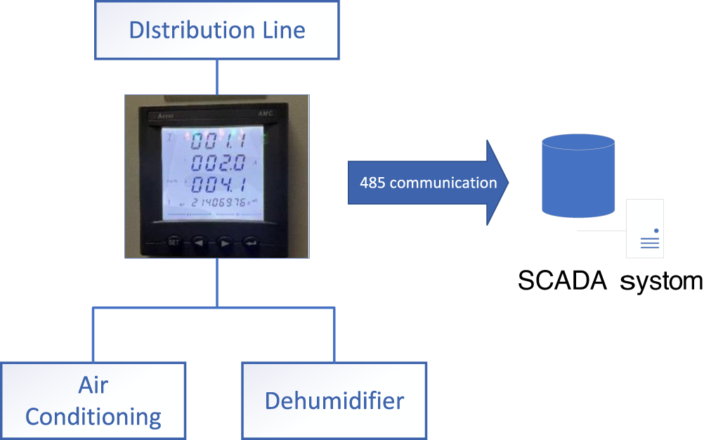
Figure 1: Data acquisition flow chart

The dataset contains minute-level sampled data from 11:00 on 08 January 2024, to 23:59 on 31 July 2024. To handle the issue of a small number of missing values, linear interpolation was used to complete the data, which was then integrated into a coherent dataset at 30-min intervals (as shown in Fig. 2). The air-conditioning load dataset X contains a total of 9866 time points, with the training set for the experiment including 8879 time points, the validation set including 1974 time points, and the test set including 986 time points.

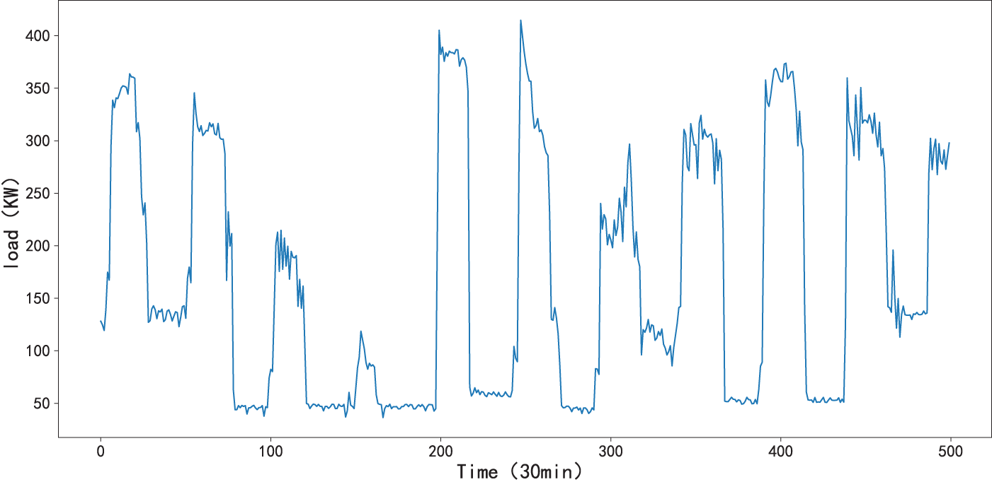
Figure 2: Partial display of air-conditioning load dataset

2.2 Data Correlation Analysis

To determine whether a robust correlation exists between historical load data and future air-conditioning load, we perform a correlation check on the dataset using the autocorrelation coefficient [29]. The calculation formula is as follows:

∑i=1n−h(xi−μ^)(xi+h−μ^)∑i=1n(xi−μ^)2(1)

xi represents the i-th observation value in the time-series data. μ^ is the mean value of the time-series data. n represents the number of samples in the time-series, and h is the lag number, which indicates the time interval between observation values. We calculated the autocorrelation coefficients for lags 1 to 10 on our dataset (Fig. 3). As can be observed, the correlation coefficients are consistently high.

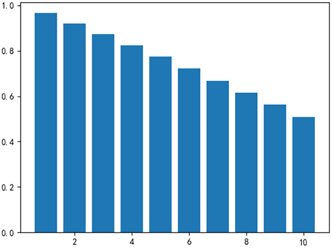
Figure 3: Autocorrelation coefficients of load data at lags 1 to 10

2.3 Analysis of Distribution Shift in Air-Conditioning Load Dataset

In time series prediction tasks, distribution shift is divided into two types: between different historical windows, and between historical windows and prediction windows. To examine whether distribution shift exists in the air-conditioning load data in these two aspects, this paper conducts a analysis on the intraspace, input space, and output space of the data.

1)   Intraspace distribution shift analysis

We randomly select 5 groups of historical windows from the dataset and plot their mean and variance, as shown in Fig. 4. It can be observed that there are significant differences in the mean and variance among different historical time windows; therefore, there exists a distribution shift between different historical time windows in this dataset.

2)   Analysis of Distribution Shift between Input Space and Output Space

To verify the presence of a distribution shift between the input space and the output space of the dataset, five different sample groups were randomly selected. There are significant differences in the means between the historical window and the prediction window of each sample in Fig. 5. This indicates that there is a distribution shift between the historical window and the prediction window across different samples.

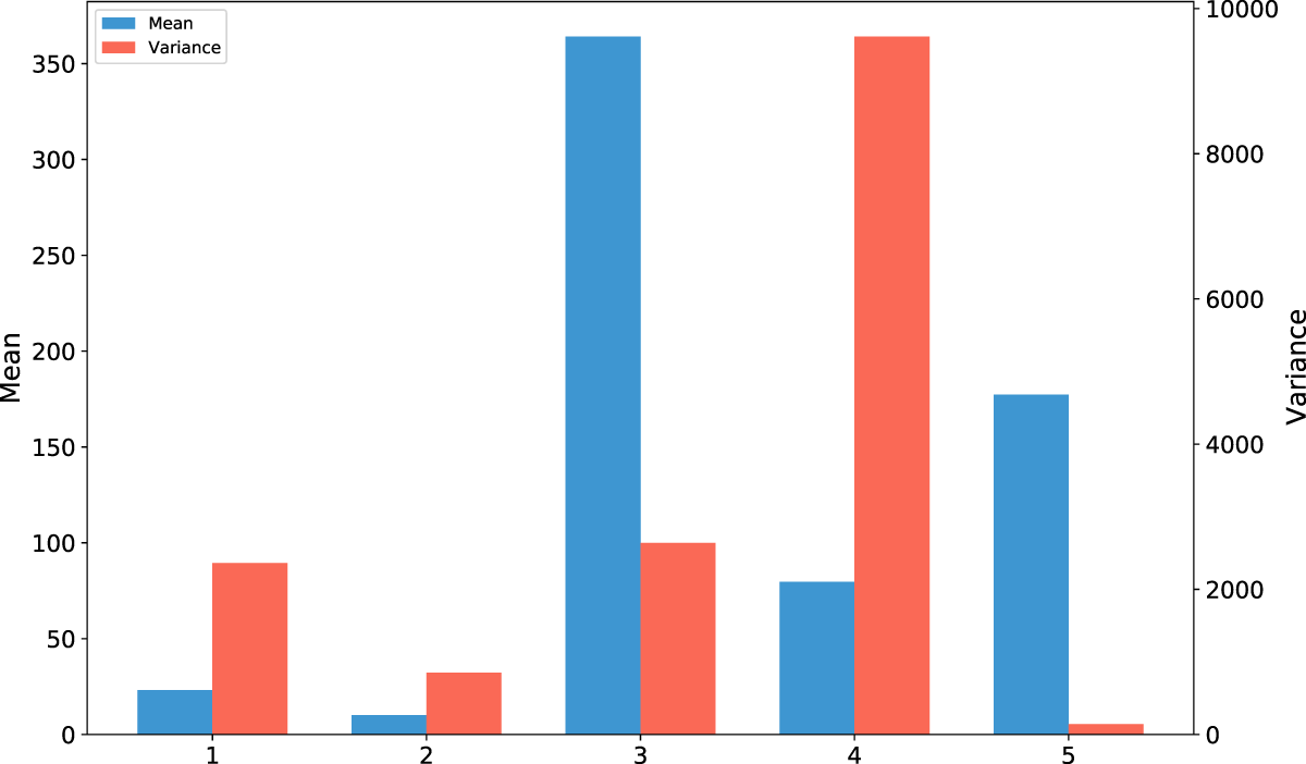
Figure 4: Mean and variance plots of historical windows from different samples

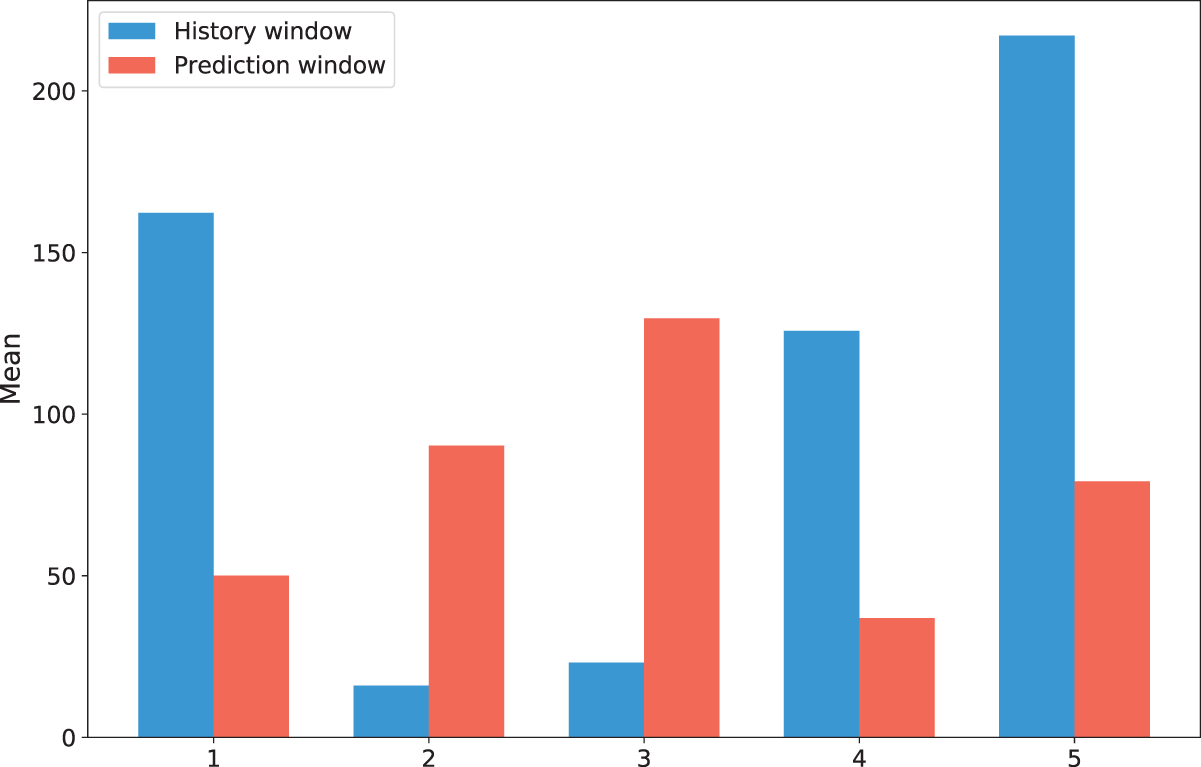
Figure 5: Mean bar charts of input space and output space for different samples

3  Proposed Method

In this study, we propose a novel hybrid method, DS-Kansformer, for predicting future air-conditioning loads. As illustrated in Fig. 6, the proposed DS-Kansformer method primarily consists of two components: the DS module and the Kansformer module. First, the DS module self-learns the mean and variance required for standardization and standardizes the time-series data of air-conditioning loads. This effectively reduces the impact of distribution shift on the prediction accuracy of the model. The standardized data Xen is then fed into the Kansformer module for processing. In the feature extraction stage, CNN Embedding and Positional Encoding are innovatively combined to obtain time-series feature information. Subsequently, the encoder processes the input features. The decoder receives the output of the encoder and its own input. Notably, to enhance the model’s ability to capture the non-linear features of the data, this paper replaces the Feed-Forward Layer in the Encoder and Decoder of the traditional Transformer with the KAN. Then, the Decoder gradually generates the output sequence and uses the Linear layer for dimensionality reduction to obtain the output Y. Finally, the output Y is passed through the De-Standardization layer of the DS module to restore the original data distribution, yielding the final prediction result Pre. The specific composition structure and technical details of each module will be elaborated in the following sections.

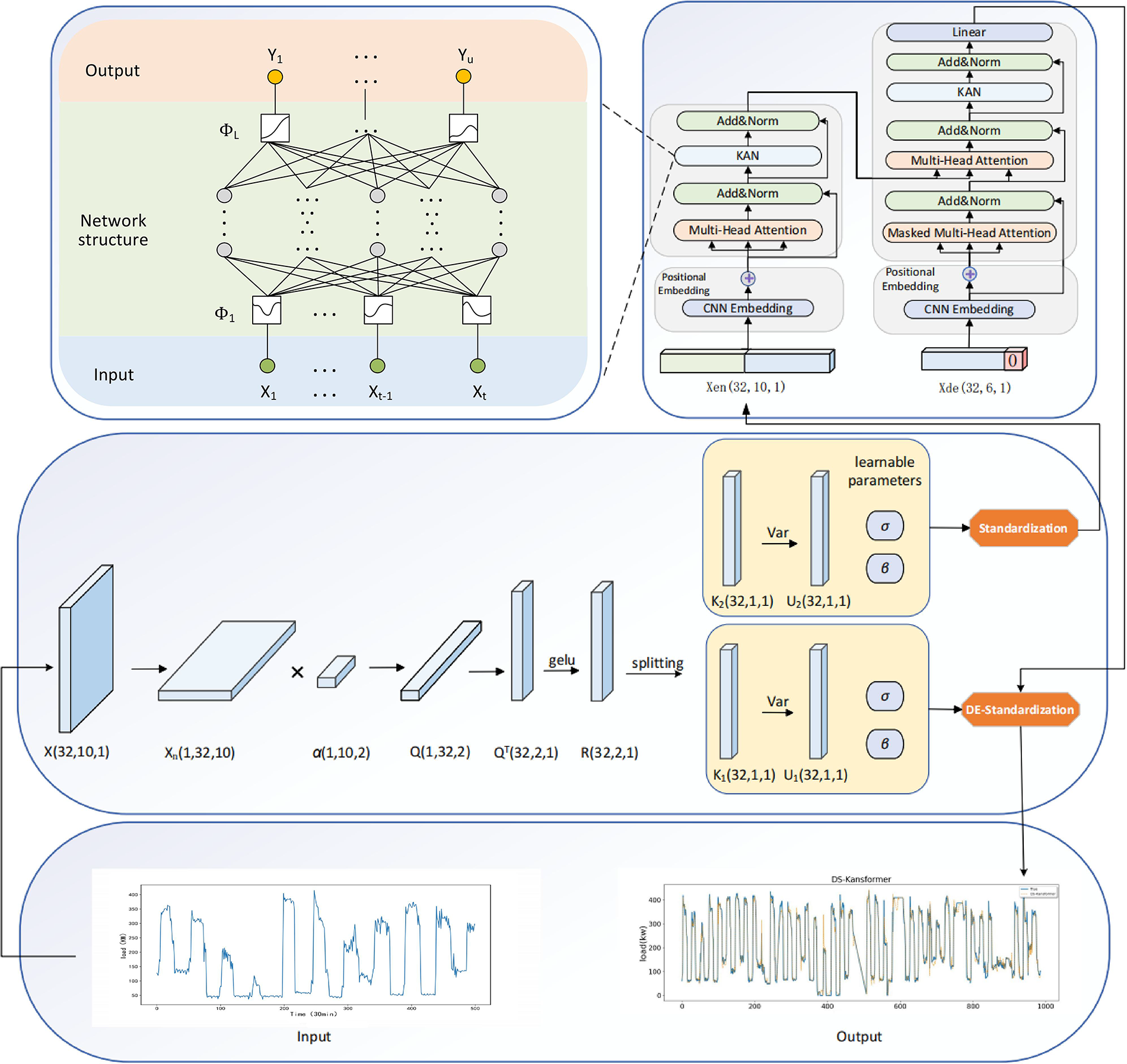
Figure 6: Overall structure diagram of the DS-Kansformer model

3.1 Composition Structure of DS Module

The DS module is introduced to enhance the model’s adaptability to distribution shifts. It effectively mitigates interference caused by distribution discrepancies occurring both within historical windows of air-conditioning load data and between historical and prediction windows, thereby improving the prediction accuracy of the Kansformer module. As shown in Fig. 7, the DS module operates through a two-stage process, which will be detailed in the following section.

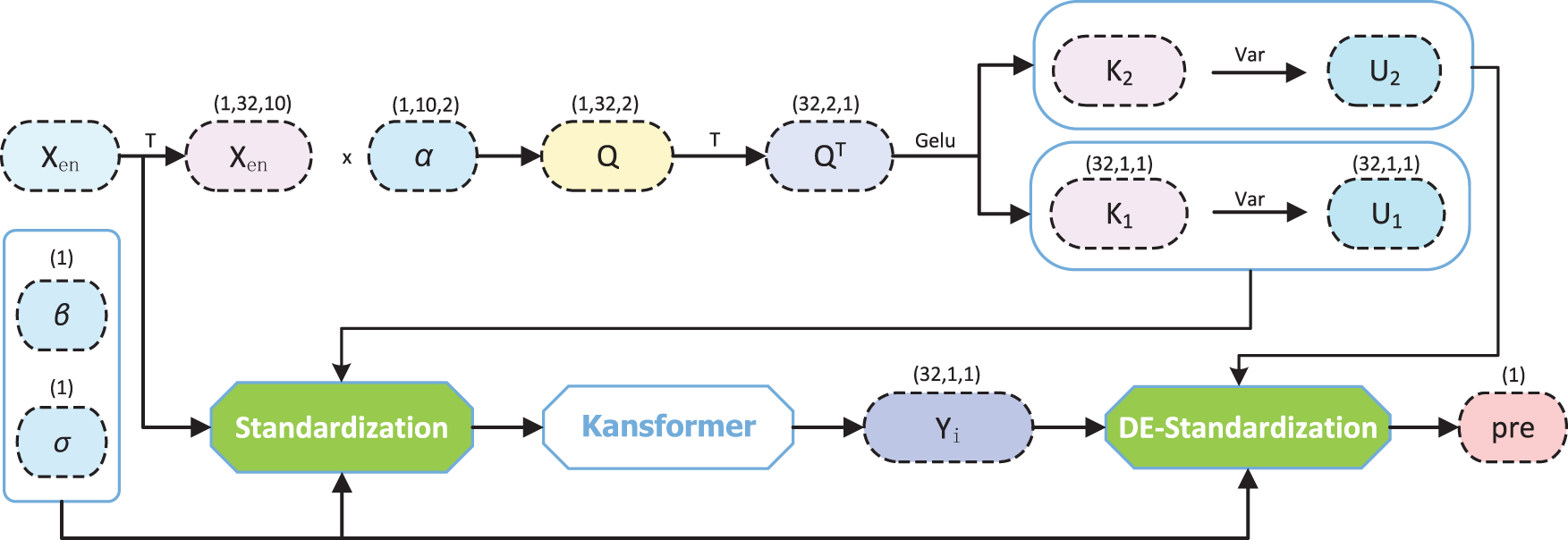
Figure 7: Structure diagram of the DS module

3.1.1 Standardization Layer

As shown in Fig. 7, where Xen represents the historical window, and its dimension is (32, 10, 1). The Batch_Size dimension is 32; the time step dimension of the historical window is 10; the dimension of the number of variables in the historical window is 1. The specific steps are as follows: First, permute the Batch_Size dimension and the time step dimension of Xen, so as to output XenT with a dimension of (1, 32, 10); second, multiply XenT by the learnable parameter α with a dimension of (1, 10, 2), so as to obtain Q with a dimension of (1, 32, 2); then permute the dimensions of Q to obtain QT with an output dimension of (32, 2, 1); next, split QT along the second dimension, so as to obtain the means K1, K2 required for standardization and inverse standardization; after that, use the means K1, K2 to calculate the variances U1, U2; finally, standardization calculation is performed with the trained learnable parameters β and σ obtained from training, and the formula is as follows:

X1=Xen−K1U1+e−8(2)

X0=βX1+σ(3)

where β is a scale coefficient and σ represents a level coefficient.

3.1.2 DE-Standardization Layer

In Fig. 7, the standardized data obtains the prediction result Yi through the Kansformer module. Subsequently, Yi, the mean value K2, the variance U2, and the learnable parameters β and σ are input into the de-standardization layer. The purpose of the de-standardization layer is to learn the mean and variance required for de-standardization from the historical window, instead of using the fixed mean and variance in the historical window for de-standardization of the prediction window, thereby reducing the impact of internal and external distribution shift problems on the prediction results obtained during de-standardization. The calculation formula is as follows:

Pre=(Yi−σ)β×U2+e−8+K2(4)

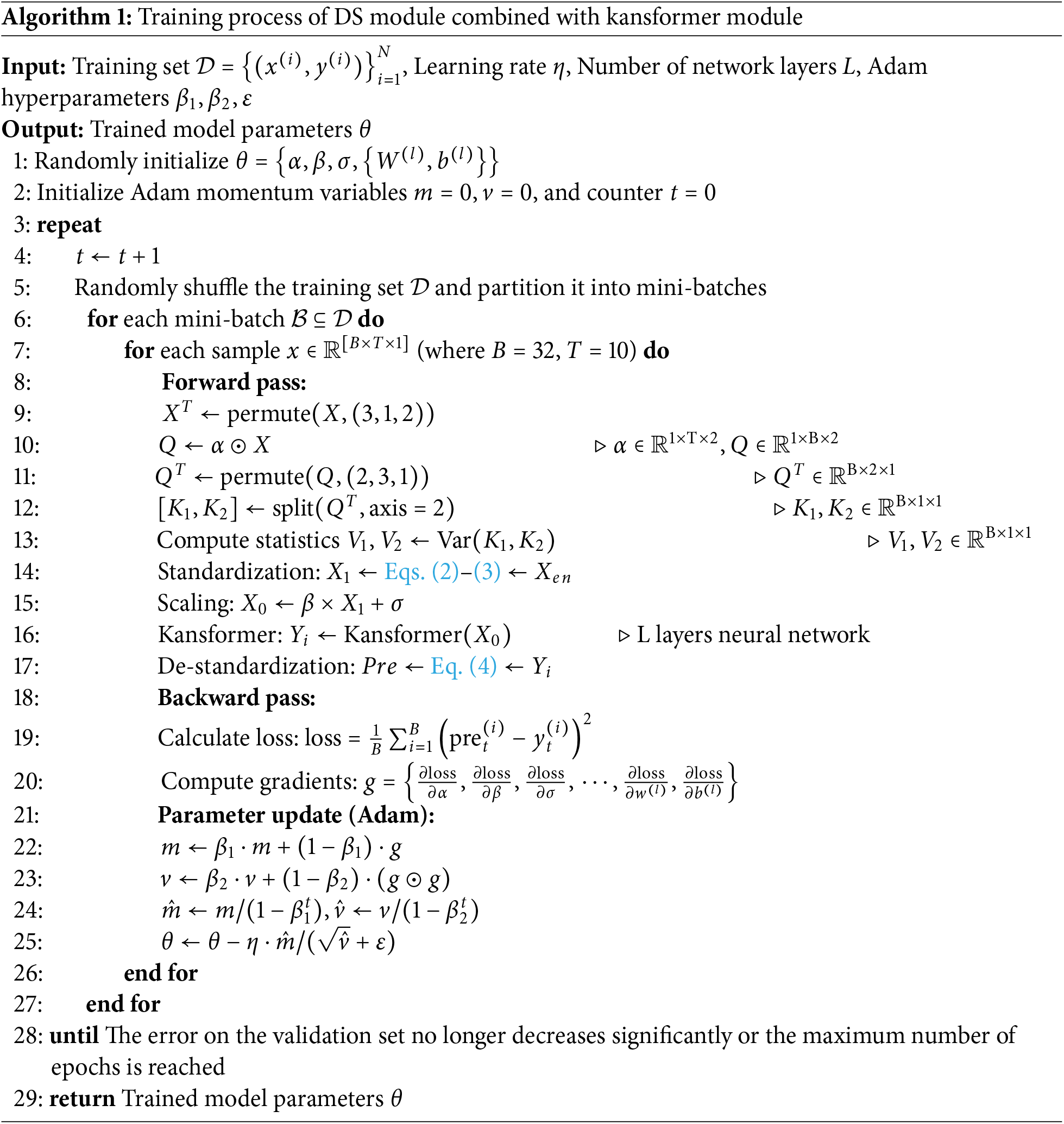
3.1.3 Learning Process of DS Module

The DS module is designed to be fully integrated into the deep learning framework. Its standardization and de-standardization layers are connected to the input and output of the Kansformer module, respectively, forming the integrated DS-Kansformer model. The detailed learning procedure is outlined in Algorithm 1. The learnable parameters in the DS model are denoted by α, β, and σ. The Kansformer consists of L layers in total, and its parameters are denoted by {W(l),b(l)}. Combining these, the final learnable parameters of the model are θ={α,β,σ,{W(l),b(l)}}. The entire training process starts with loading 32 samples from the training set. The historical window is fed into the normalization layer of the DS model to obtain the normalized historical window X0, which is then input into the Kansformer model for prediction, generating the prediction result Yr. This result is further processed by the denormalization layer of the DS model to produce the final prediction result Pre. The loss is calculated between this prediction result and the true value, yielding the loss values for the 32 samples. Backpropagation is applied to these losses to obtain gradients, which are then fed into the Adam optimizer to update θ once. This process is repeated until the model converges, resulting in the final θ, which includes α,β,σ from the DS model as well as all layer weights and bias parameters of the Kansformer.

3.2 Kansformer Module

After the DS module processes the data with distribution shift, the obtained data Xen is used as the input of the Kansformer module. The specific structure of the Kansformer module is shown in Fig. 8. The Kansformer module is composed of an Encoder and a Decoder. In the Encoder, it includes an Embedding layer, a multi-head attention layer, a KAN layer, and two Add&Norm layers. The structure of the Decoder is similar to that of the Encoder. However, it is worth noting that, in order to prevent the model from paying attention to the information of subsequent positions at the current position during training, a mask is used to set the future information to 0. Therefore, the input Xde of the Decoder is composed of the last five time steps of Xen and 0 values with the length of the prediction.

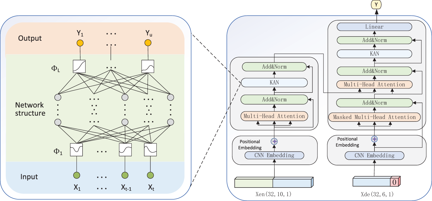
Figure 8: Structure diagram of the Kansformer module

As established in Section 2.2, each data point in the air-conditioning load time series is not isolated; the surrounding information significantly contributes to understanding its intrinsic characteristics and underlying patterns. To enhance the model’s ability to characterize short-term local patterns, this study adopts a one-dimensional CNN (1D-CNN) for sequence embedding. It introduces inductive biases of local translation invariance and denoising, which can improve the perception of sudden changes and periodic fragments. Moreover, weight sharing enables more stable training and fewer parameters when working with small to medium-sized samples. In terms of dimension setting, the convolution kernel size is set to 3, which ensures that the receptive field covers short-term dynamics without excessive smoothing. The input format is (32,10,1), which is first transposed to (32,1,10) to match the input format of the 1D-CNN. After convolution, the output format becomes (32,dmodel,10). Finally, the output is restored to (32,10,dmodel) with surrounding information fused, and then combined and added with positional encoding. Positional encoding is used to represent the position of the current data and the distance between different data points. The formula is as follows:

PEpos,2i=sin⁡pos100002idmodel(5)

PEpos,2i+1=cos⁡pos100002idmodel(6)

where pos denotes the position index of the data point, i denotes the data dimension, and dmodel denotes the dimension of the model.

The next encoder utilizes the multi-head self-attention mechanism to synthesize and extract the information of the whole sequence, specifically, the input Xeni representation is divided into h heads, and each attention head independently processes the three parameters of query, key, and value. After that, the results are combined to get the information feature XenH that fuses the different perspectives, and the attention computation formula is as follows:

Attention(Q,K,V)=softmax(QKTdkV)(7)

headj=Attention(QWjQ,KWjK,VWjV)(8)

MultiHead=concat(head1,…,headg)WU(9)

where WjQ∈Rdmodel×dq,WjK∈Rdmodel×dk,WjV∈Rdmodel×dv are the independent weight matrices of each head, dq, dk, dv denote the dimensions of each head, WU∈Rhdv×dmodel is the spliced linear transformation matrix, 1dk is the scaling factor, T is the time step length, and dmodel is the feature dimension of each time step.

After obtaining the output of self-attention, the Add&Norm layer is entered immediately after, enabling the model to learn useful features more easily, preventing information loss as well as being more stable and converging faster during training. Next, we the introduction of KAN replaces the traditional feedforward layer for further feature extraction and transformation.

The Kolmogorov-Arnold theorem allows the task of learning a high dimensional function to be reduced to learning a polynomial one-dimensional function. Specifically, any function that depends on x=[x1,x2,…,xn] of a multivariate continuous function f(x) can be represented on a bounded domain of definition by a finite composite of continuous functions involving only one variable. KAN is based on this theory, and the structure behaves as a stack of L layers of nonlinear transformations.

Fig. 9a and b shows the network structures of KAN and MLP, respectively. It can be observed that KAN features a novel neural network structure: it replaces the linear weights in the Feed-Forward Layer with learnable spline-based univariate activation functions, which enables efficient approximation and representation of complex nonlinear relationships. This approach—subversively modifying the computational method of the Feed-Forward Layer by embedding learnable parameters into the activation operation—helps the model efficiently model nonlinear features with fewer parameters. The neural network of KAN is expressed as follows:

KAN(XenL)=ΦL−1∘ΦL−2⋯Φ0∘XenL(10)

where XenL is an input feature and Φi is a univariate function on the edge, we parameterize the residual activation function ϕ(x) by using a linear combination of the LeakyReLu activation function and the spline function as follows:

ϕ(x)=ωb(LeakyReLu(x)+spline(x))(11)

LeakyReLU(x)=f(x)={x,if x≥0δ⋅x,if x<0(12)

spline(x)=∑iciBi(x)(13)

where the value of δ is 0.01, Bi(x) is a B-spline basis function defined on a grid to represent any univariate function over a finite domain that has the same shape but different locations, ci is a control coefficient for B-spline shaping, and the LeakyReLU function, which enhances the smoothness of the unitary function, ωb is a weight parameter, and the network utilizes this structure to extract the features that merge the nonlinear representations.

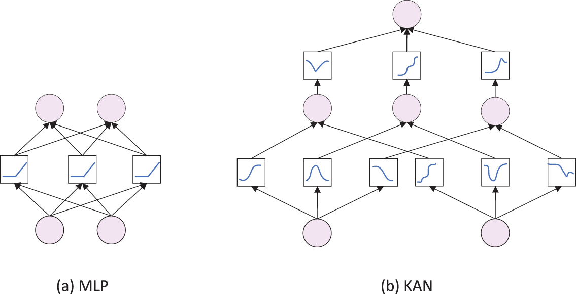
Figure 9: Network structure of KAN and MLP

KAN network architecture is shown in Fig. 10, where it can be seen that the learnable activation functions are represented in a box, the ci parameter controls the amplitude of each B-spline, and the summation of multiple B-spline functions yields the spline function, which, in this study, is used 3 times with a B-spline and a grid size of 5. The KAN utilizes the combining and superposition of univariate functions that can efficiently approximate and represent complex nonlinear relationships. This greatly improves the nonlinear feature representation of the model. Then the output features of the KANs are connected with the input features through residual connection and processed by Layer Normalization. Then, the processed results are fed into the decoder part, which has the same structure as the encoder. Note that the decoder adopts Masked Multi-Head Attention, using masking to prevent the current position from focusing on subsequent positions’ information, thus ensuring the autoregressive property. The Encoder-Decoder Attention layer utilizes the Multi-Head Attention mechanism to receive the information from the encoder’s output as well as its own input to fuse the contextual information.

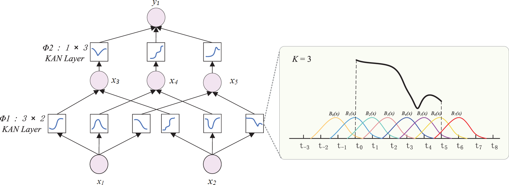
Figure 10: KAN network architecture

Finally, the output of the decoder is passed through the Linear and Softmax layers to obtain the output Yi. In the computation of loss stage it is necessary to compute the loss using the original data distribution so that the model can accurately identify the difference between the predicted and actual values. Therefore, it is necessary to perform DE-standardization on the predicted value Yi output from the Kansformer module in order to restore the original distribution of the data.

4  Experimentation and Analysis

This section introduces specific experimental methods, including the dataset, evaluation metrics, and settings for training the model. The model prediction task is to predict the air-conditioning load power value for the next 30 min using the historical sequence of the past 5 h. To verify that DS-Kansformer has excellent prediction performance, hyperparameter analysis, ablation experiment analysis, and comparative experiment analysis are carried out on it in this section.

4.1 Evaluation Metrics and Experimental Setup

4.1.1 Evaluation Metrics

In order to better compare the overall performance of each model, three common indicators in the field of regression prediction are selected in this experiment to evaluate the proposed prediction model. They are MAE, RMSE and R2, respectively, and the calculation formulas are as follows:

MAE=1n∑i=1n|y^i−yi|(14)

RMSE=1n∑i=1n(y^i−yi)2(15)

R2=1−∑i=1n(y^i−yi)2∑i=1n(y¯−yi)2(16)

where y^i denotes the predicted value of the i-th sample, yi signifies the actual value of the i-th sample, y¯ represents the mean value of the actual observed values.

4.1.2 Experimental Setup

The experiments in this paper were conducted on a system equipped with a deep learning GPU (Nvidia RTX2070), using the PyCharm development environment and Python version 3.8.2. Hyperparameters are parameters that need to be preset before training a machine learning model, which directly affect aspects such as the model’s training process and structural complexity. The DS-Kansformer model proposed in this paper is mainly influenced by dmodel/nheads and the number of encoder layers. Below, we will conduct hyperparameter analysis focusing on these three factors based on the collected air-conditioning load dataset.

dmodel/nheads need to be adjusted synergistically to balance performance and efficiency. Therefore, we set four different groups of parameters to compare their performance (Fig. 11). When dmodel/nheads is 512/8, the MAE and RMSE reach the minimum values, while R2 reaches the maximum value.

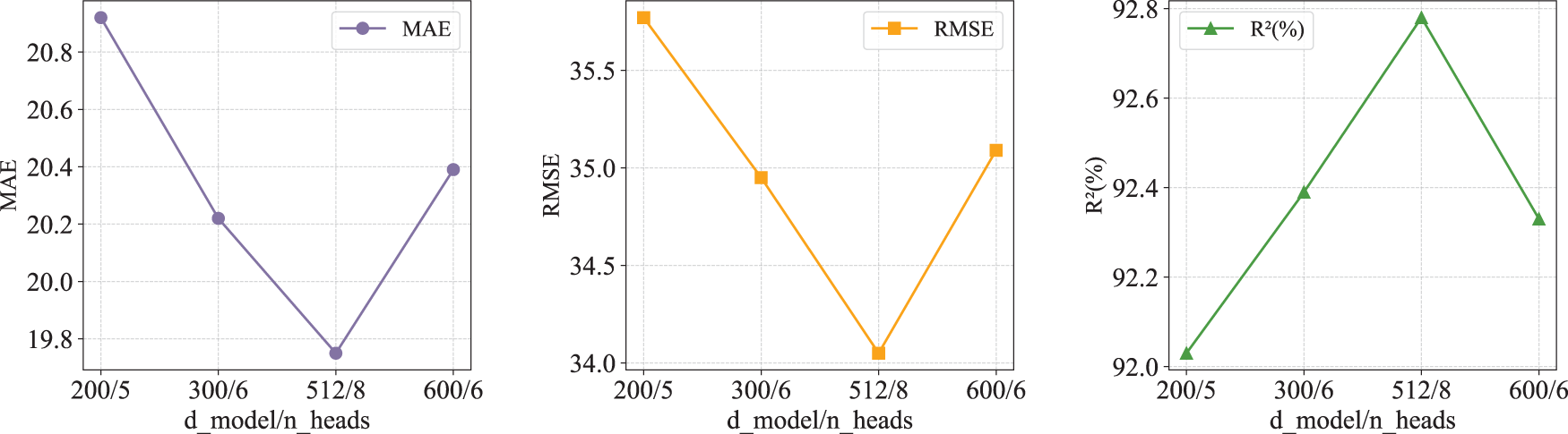
Figure 11: Performance under different d_model/n_heads

The encoder_layers has an important impact on the model’s performance, computational efficiency, and generalization ability. Therefore, tests and comparisons were conducted on the number of layers, as shown in Fig. 12. When the cumulative number of encoder layers in the DS-Kansformer model reaches 3, the MAE and RMSE are at their minimum values, and R2 is at its maximum value. Therefore, the value of encoder_layers is set to 3.

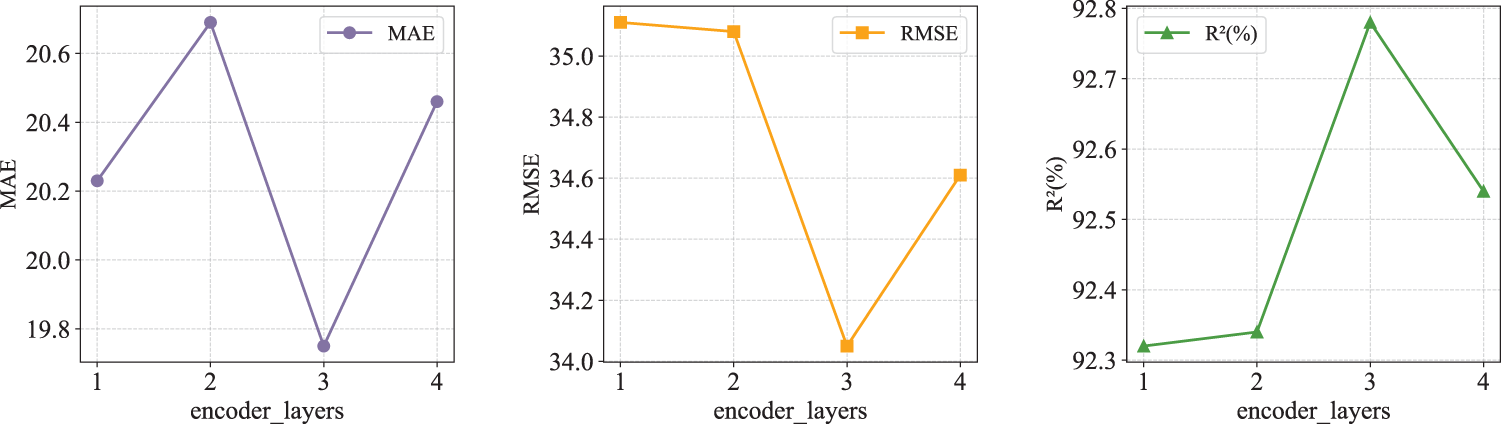
Figure 12: Performance under different d_model/n_heads

The core hyperparameters of KAN include grid_size, spline_order, and the type of basis functions. Considering that grid_size and spline_order have been fully validated in the official implementation, and improper parameter settings may affect fitting stability and generalization performance, this paper chooses not to tune these two parameters and directly adopts their default values. The selection of smoothing function types will be analyzed in the ablation experiments of Kansformer.

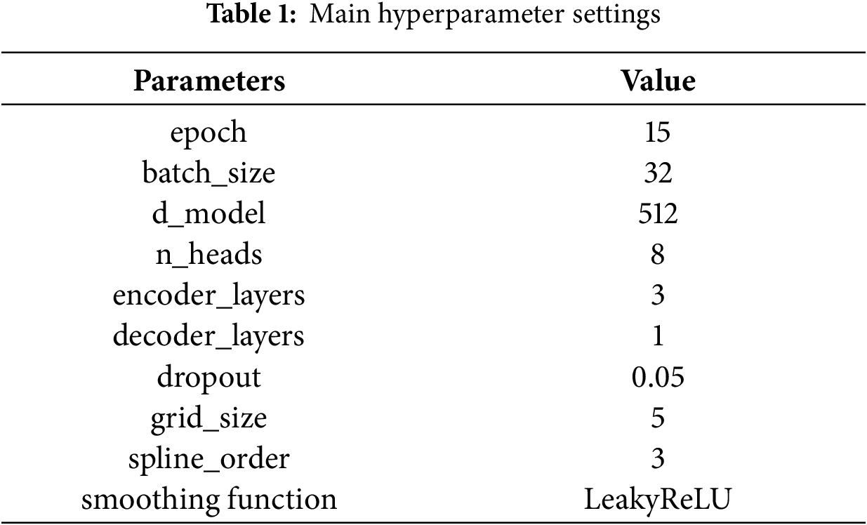
The main hyperparameter settings finally determined are showed in Table 1.

The hyperparameter configurations of each comparative model are shown in Table 2.

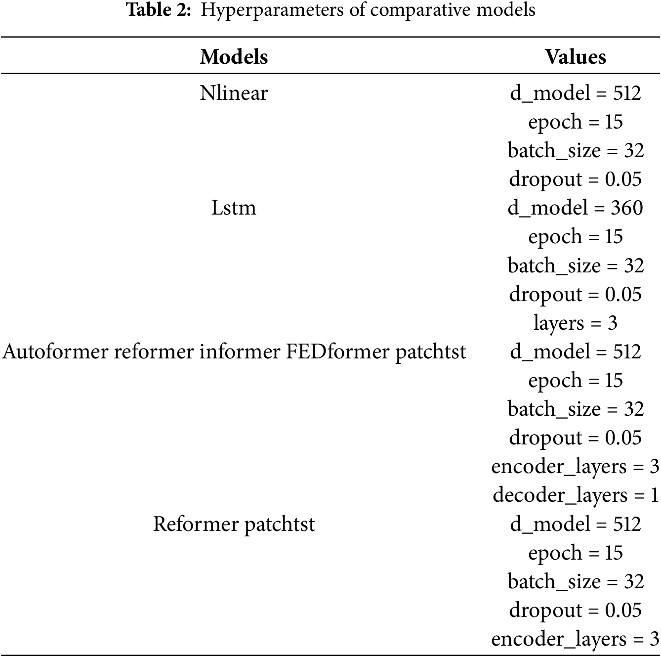
To ensure the fairness of the experiment, models based on the Transformer architecture adopt consistent hyperparameter settings. For other models, reasonable hyperparameter configurations are also applied. This ensures that all models are fully capable of learning complex patterns, thereby objectively reflecting the performance differences between different models.

4.2 Ablation Experiment

To study the impact of different modules in the DS-Kansformer model on the overall model performance, this section will conduct ablation experiment analysis on the DS module and the Kansformer module, respectively.

4.2.1 DS Ablation Experiment

To verify that the DS module can effectively reduce the negative impact of the distribution shift problem of air-conditioning load power data on the time-series prediction model, and to verify that the self-learning parameters in the standardization layer and de-standardization layer of the DS model have more advantages than fixed parameters, we carry out the DS ablation experiment analysis. The specific experimental data are shown in Table 3.

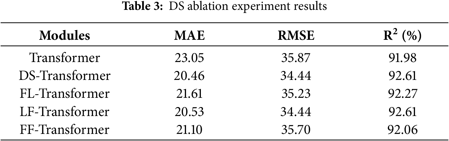
FL represents the fixed standardization layer with the learnable de-standardization layer, LF represents the learnable standardization layer with the fixed de-standardization layer, and FF represents the fixed standardization layer with the fixed de-standardization layer. First, compared with Transformer, DS-Transformer, FS-Transformer-LDS, LS-Transformer-FDS, and FS-Transformer-FDS all exhibit lower MAE and RMSE values along with higher R2 values. This further verifies that air conditioning load power data can degrade the prediction performance of Transformer models. Both learnable and non-learnable fusion methods can, to a certain extent, address distribution shift issues and improve the prediction performance of Transformer models. Second, compared with the FS-Transformer-LDS model, DS-Transformer shows reduced MAE and RMSE along with improved R2, which verifies the contribution of the normalization layer in the DS model. It demonstrates advantages in reducing internal spatial distribution shifts through self-learned normalization means and variances. When comparing DS-Transformer with the LS-Transformer-FDS model, they exhibit equal MAE and RMSE, but DS-Transformer achieves a higher R2, verifying the contribution of the denormalization layer in the DS module. This confirms its advantages in reducing both internal and external spatial distribution shifts through self-learned denormalization means and variances. Among DS-Transformer, FS-Transformer-LDS, and FS-Transformer-FDS, DS-Transformer achieves the lowest MAE and RMSE along with the highest R2, demonstrating that the learnable mean and variance form has advantages over fixed mean and variance.

4.3 Kansformer Ablation Experiment

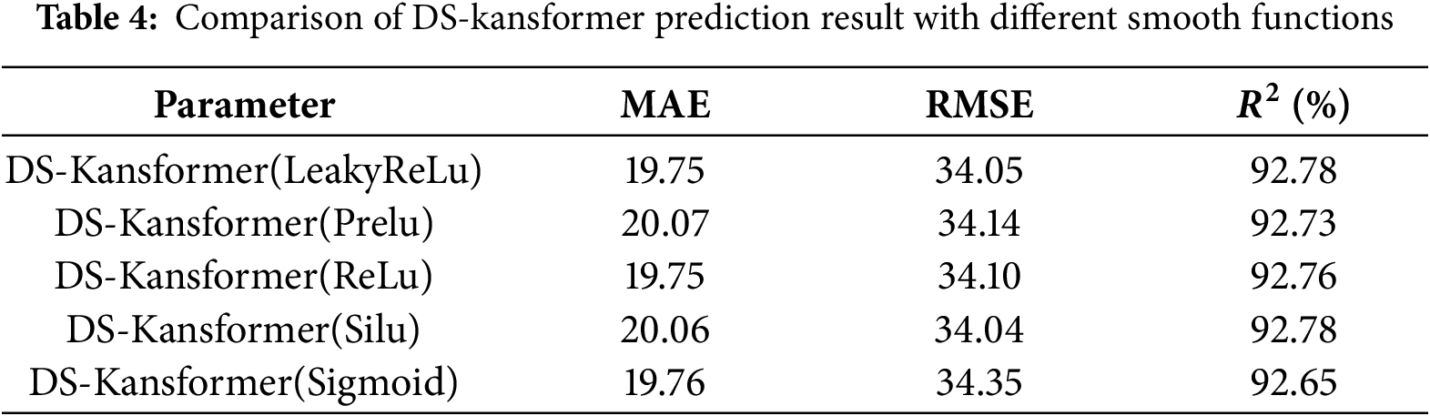
The original KAN network uses the SiLU activation function for smoothing, but in experiments on real air-conditioning load datasets, it is found that different activation functions have a great impact on performance. It can be seen from Table 4 that the LeakyReLu smoothing function has the best comprehensive performance. Compared with smooth activation functions such as SiLU and Sigmoid, LeakyReLU can avoids the vanishing gradient problem and ensures training stability, and it does not incur the computational overhead associated with the exponential operations required by smooth functions like SiLU and Sigmoid.

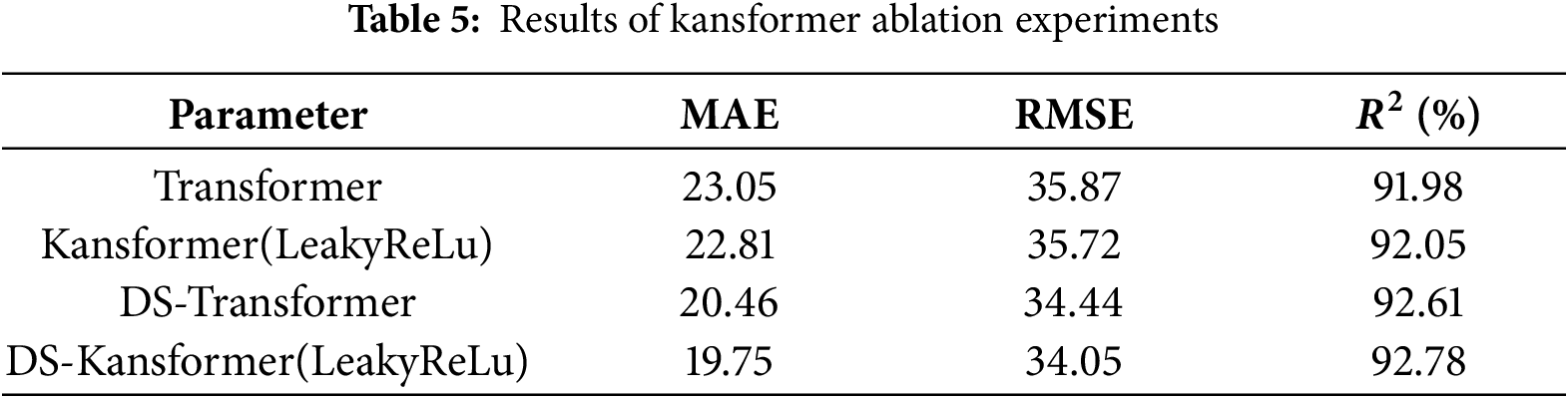
The optimal smoothing function LeakyReLu was used as the smoothing function for the KAN network in the Kansformer module to conduct ablation experiments on the Kansformer module. Some randomly selected prediction results are visualized in Fig. 13, which shows that regardless of whether the DS module is added or not, the prediction curve of the Kansformer model using the KAN network is closer to the real curve than that of the Transformer. Table 5 further verifies that the Kansformer model can effectively enhance the model’s ability to express nonlinear features, thereby making the prediction results more accurate.

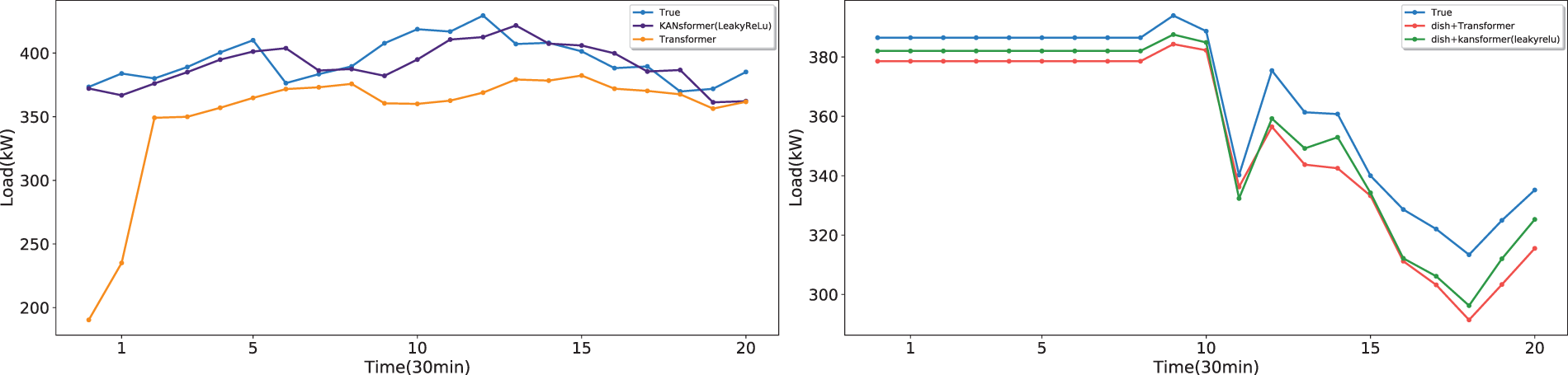
Figure 13: Comparison chart of kansformer module ablation experiments

4.4 Comparative Experiment

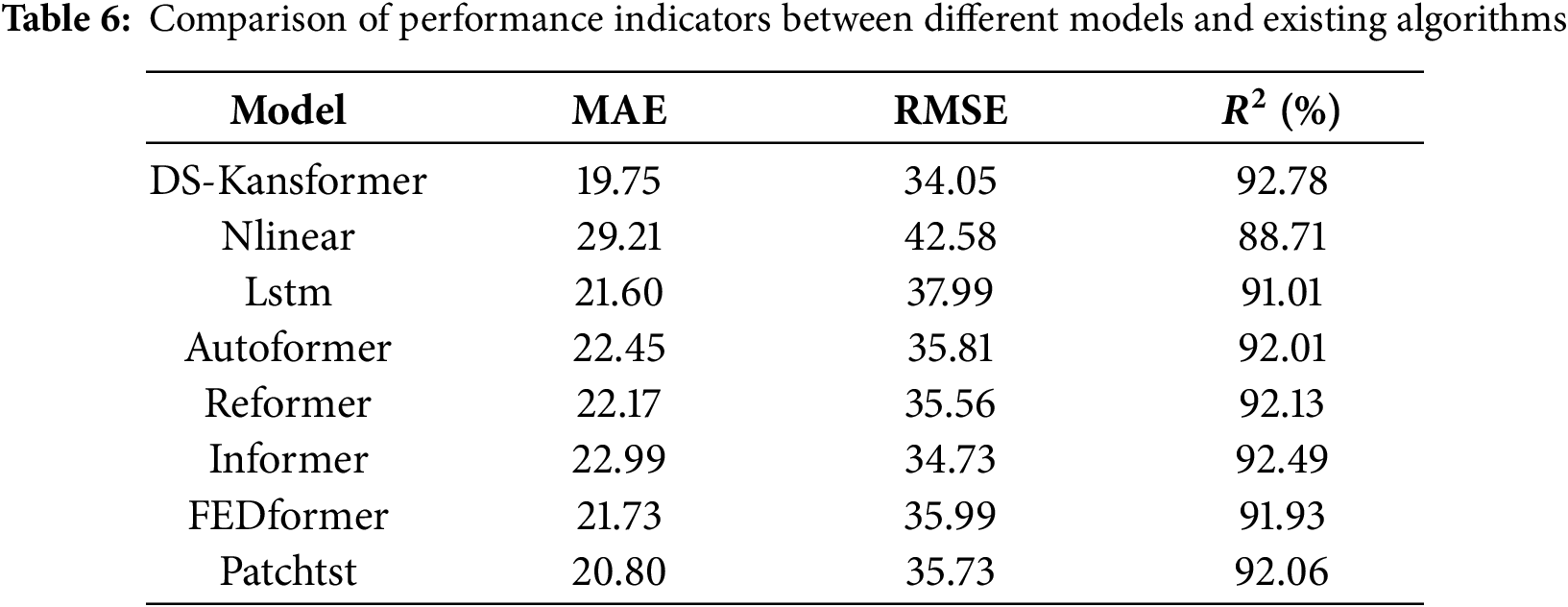
To prove that the DS-Kansformer model proposed in this paper has better prediction performance than common time-series prediction models, we conducted a comparative analysis of DS-Kansformer with existing algorithms such as Lstm and Autoformer based on the collected air-conditioning load dataset. The prediction results of each model on the test set are shown in Fig. 14. For a more intuitive comparison with the prediction results of other models, we randomly selected prediction results from a continuous 5-h period (Fig. 15). It can be seen that the linear model Nlinear has a large deviation between its prediction curve and the actual values, which indicates that linear models have certain limitations in capturing the trend changes of data. In addition, LSTM and other Transformer-based models still have certain errors in predicting some load values. Compared with other models, the prediction curve of the DS-Kansformer model has the highest degree of consistency with the real curve and can fit the load change trend to the greatest extent.

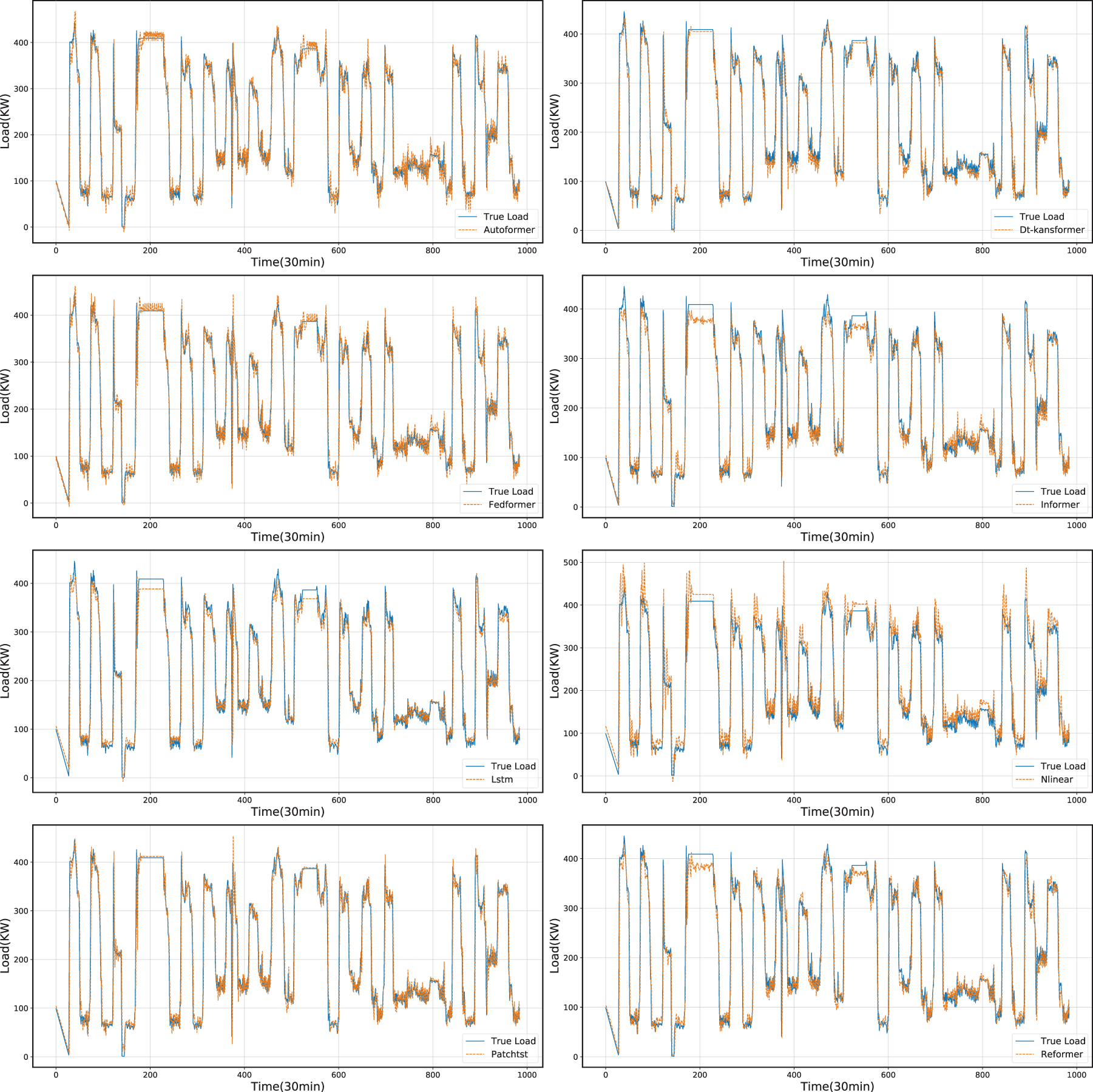
Figure 14: Comparison between predicted values and actual values of different models

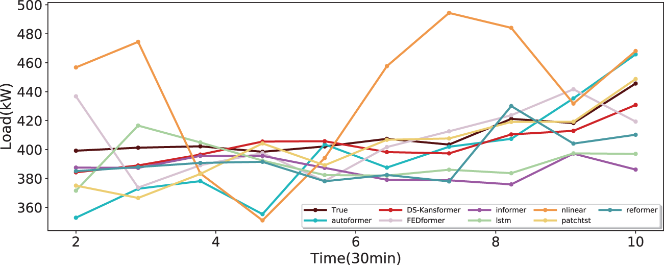
Figure 15: Comparison of different models within a continuous time period (5h)

To more accurately evaluate the performance of the DS-Kansformer model, we used MAE, RMSE, and R2 as evaluation metrics to compare it with different models, and the comparison results are shown in Table 6. It can be seen that the linear model Nlinear performs the worst, which proves that the disadvantage of linear models in being difficult to capture complex nonlinear patterns will affect the prediction effect of the model. As a time-series model, the LSTM model has better performance results than NLinear. Autoformer, Reformer, Informer, FEDformer, and Patchtst are all algorithms based on the Transformer architecture. The self-attention mechanism they adopt can better adapt to the characteristics of time-series data and perform well in predicting air-conditioning loads. In contrast, DS-Kansformer shows the best performance in the performance evaluation, with MAE, RMSE, and R2 being 19.75, 34.05, and 92.78, respectively. Compared with the sub-optimal algorithm Informer, the MAE and RMSE of the DS-Kansformer model proposed in this paper are reduced, and R2 is improved, which proves that the method proposed in this paper can effectively improve the prediction accuracy and model fitting ability by enhancing the model’s nonlinear fitting ability and alleviating the problem of distribution shift.

To ensure that the research not only focuses on performance accuracy but also takes into account the timeliness requirements in practical applications, we measured the average inference time of each model on the test set. As can be seen in Table 7, the average per-sample inference time of our model has reached 14.18 ms, which is close to the inference time of most comparative models. This fully enables it to meet the requirements for prediction response speed in real-world scenarios. Meanwhile, to provide a unified and comparable metric across different models, we adopt the Universal Complexity Index (UCI) as the measure of computational complexity, with its formula presented as follows:

UCIfwd/sample=ϕP+ω(LeffDmodelLayersest)(17)

Leff=seq_len+label_len+pred_len(18)

where P is the number of trainable parameters; Leff represents the number of effective tokens involved in one forward pass; seq_len, label_len, and pred_len represent the historical sequence length, label length, and prediction length, respectively; Dmodel is the channel width; Layersest is the estimated effective number of layers; ϕ and ω are set to 1. the term ϕP reflects the parameter-state complexity; the term ω(LeffDmodelLayersest) approximately reflects the activation scale of one forward processing.

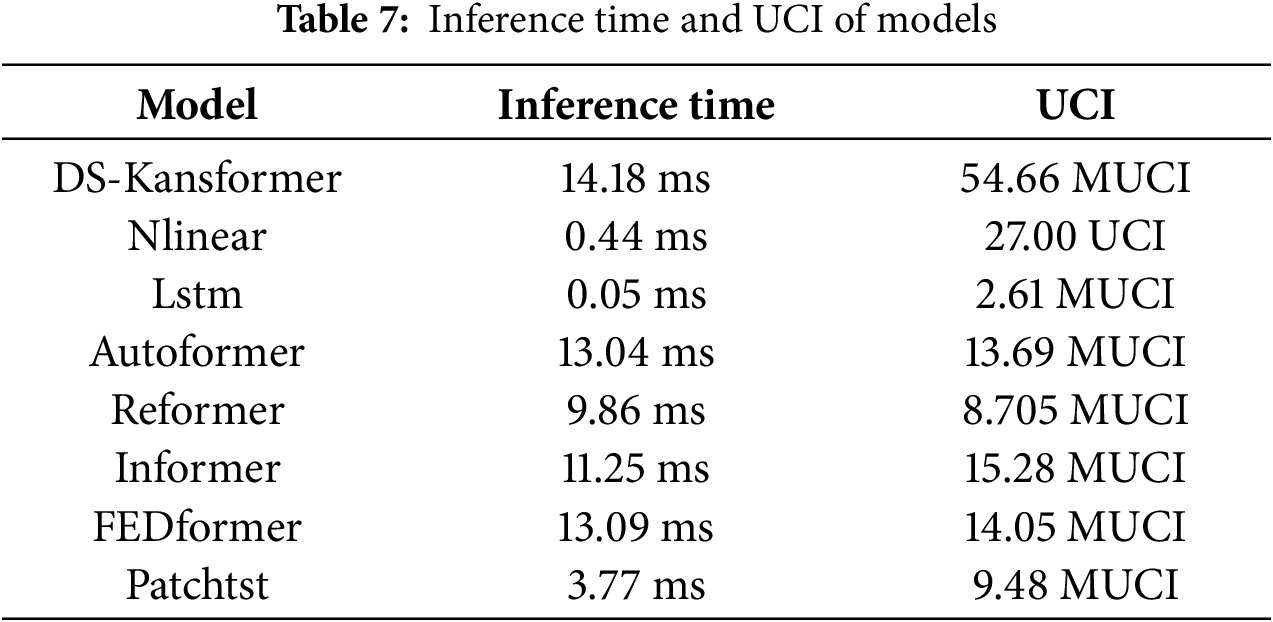
As can be seen from Table 7, compared with other models, our model does have higher computational complexity, which leads to slower training speed in the training phase. The reason is that the KAN layer involves basis function expansion and backpropagation of piecewise gradients, and its backward complexity is higher than that of the standard MLP layer. However, its forward path can be highly vectorized, so the latency gap between our model and the comparative models on the inference side is very small. Nevertheless, training is only an offline, one-time upfront investment in the early stage. From the perspective of the core goal of our model research, the ultimate purpose is still to improve prediction accuracy and ensure that the inference speed meets the requirements of practical deployment. Certainly, although our current method has improved accuracy, there is indeed room for optimization in terms of computational complexity. In the future, we will explore lightweight improvements to the model to better adapt to tasks in different practical application scenarios.

5  Conclusion

Based on the air-conditioning load dataset of a large-scale multi-functional building in Xiamen, this paper addresses the issues of distribution shift in air-conditioning load data and insufficient nonlinear representation of Transformer models, and constructs an air-conditioning load prediction model—DS-Kansformer. Through the collaborative combination of modules, this model effectively tackles the core challenges in the field of building air-conditioning load prediction: the self-learning standardization layer of the DS module aligns data distributions in the feature space, effectively alleviating the shift between the training scenario and real-world scenarios and providing a stable input foundation for the model; the KanSformer, which works in synergy with it, leverages the KAN to enhance the ability to express complex nonlinear relationships in load time series and improve interpretability, overcoming the limitations of traditional models. Finally, restoration via the DE-standardization layer ensures that the prediction results are consistent with the scale of the original data, enabling accurate load prediction. Experiments show that our model demonstrates high prediction accuracy: when predicting the next 30 min, the RMSE is 34.05, the MAE is 19.75, and the R2 is 92.78%. It outperforms other common load prediction models. Moreover, the model’s inference time is 14.18 ms, which can meet the timeliness requirements in practical applications. This proves that in practical applications, the model can provide accurate and timely prediction information for energy management and scheduling.

Meanwhile, we also recognize that there is still room for expansion and deepening in this research. Next, the research will advance from two aspects: on the one hand, we will continuously optimize the algorithm model to further enhance the model’s adaptability and generalization ability in complex data scenarios, as well as improve the model’s lightweight; on the other hand, we will focus on exploring the application scenarios of the algorithm. For instance, we will apply this method to wind power-dominated electricity markets. Given that wind power is significantly affected by environmental factors such as wind speed, wind direction, and weather, we will optimize the model’s ability to capture complex patterns. By incorporating multi-source fused features from meteorological data and historical wind power load data, we will improve the accuracy of short-term wind power forecasting, thereby providing technical support for market dispatching decisions and risk management.

Acknowledgement: The authors thank the XiaMen INESIN Control Technology Co. for the dataset.

Funding Statement: This work is supported by the National Natural Science Foundation with grant No. 12374408.

Author Contributions: Methodology, Jingjing Wen; software, Jingjing Wen; formal analysis, Qingyue Zhang; data curation, Yeting Wen; writing—original draft preparation, Jingjing Wen; supervision, Cuihong Wen and Fanyong Cheng; writing—review and editing, Cuihong Wen and Fanyong Cheng. All authors reviewed the results and approved the final version of the manuscript.

Availability of Data and Materials: The data that support the findings of this study are available from the author upon reasonable request.

Ethics Approval: Not applicable.

Conflicts of Interest: The authors declare no conflicts of interest to report regarding the present study.

References

1. Sun Y, Wilson R, Wu Y. A review of transparent insulation material (TIM) for building energy saving and daylight comfort. Appl Energy. 2018;226:713–29. doi:10.1016/j.apenergy.2018.05.094. [Google Scholar] [CrossRef]

2. Fan C, Yan D, Xiao F, Li A, An J, Kang X. Advanced data analytics for enhancing building performances: from data-driven to big data-driven approaches. Build Simul. 2021;14(1):3–24. doi:10.1007/s12273-020-0723-1. [Google Scholar] [CrossRef]

3. Avci M, Erkoc M, Rahmani A, Asfour S. Model predictive HVAC load control in buildings using real-time electricity pricing. Energy Build. 2013;60:199–209. doi:10.1016/j.enbuild.2013.01.008. [Google Scholar] [CrossRef]

4. Zhang D, Shah N, Papageorgiou LG. Efficient energy consumption and operation management in a smart building with microgrid. Energy Convers Manag. 2013;74:209–22. doi:10.1016/j.enconman.2013.04.007. [Google Scholar] [CrossRef]

5. Pérez-Lombard L, Ortiz J, Pout C. A review on buildings energy consumption information. Energy Build. 2008;40(3):394–8. doi:10.1016/j.enbuild.2007.03.007. [Google Scholar] [CrossRef]

6. Dudek G. Pattern-based local linear regression models for short-term load forecasting. Electr Power Syst Res. 2016;130(3):139–47. doi:10.1016/j.enbuild.2007.03.007. [Google Scholar] [CrossRef]

7. Gastaldi M, Lamedica R, Nardecchia A, Prudenzi A. Short-term forecasting of municipal load through a Kalman filtering based approach. In: IEEE PES Power Systems Conference and Exposition. 2004 Oct 10–13; New York, NY, USA. p. 1453–8. doi:10.1109/PSCE.2004.1397538. [Google Scholar] [CrossRef]

8. Hagan MT, Behr SM. The time series approach to short term load forecasting. IEEE Trans Power Syst. 1987;2(3):785–91. doi:10.1109/TPWRS.1987.4335210. [Google Scholar] [CrossRef]

9. Chen Y, Xu P, Chu Y, Li W, Wu Y, Ni L, et al. Short-term electrical load forecasting using the support vector regression (SVR) model to calculate the demand response baseline for office buildings. Appl Energy. 2017;195:659–70. doi:10.1016/j.apenergy.2017.03.034. [Google Scholar] [CrossRef]

10. Chae YT, Horesh R, Hwang Y, Lee YM. Artificial neural network model for forecasting sub-hourly electricity usage in commercial buildings. Energy Build. 2016;111(1):184–94. doi:10.1016/j.enbuild.2015.11.045. [Google Scholar] [CrossRef]

11. Amarasinghe K, Marino DL, Manic M. Deep neural networks for energy load forecasting. In: 2017 IEEE 26th International Symposium on Industrial Electronics (ISIE); 2017 Jun 19–21; Edinburgh, UK. p. 1483–8. doi:10.1109/ISIE.2017.8001465. [Google Scholar] [CrossRef]

12. Shi H, Xu M, Li R. Deep learning for household load forecasting—a novel pooling deep RNN. IEEE Trans Smart Grid. 2018;9(5):5271–80. doi:10.1109/TSG.2017.2686012. [Google Scholar] [CrossRef]

13. Magalhães B, Bento P, Pombo J, Calado MR, Mariano S. Short-term load forecasting based on optimized random forest and optimal feature selection. Energies. 2024;17(8):1926. doi:10.3390/en17081926. [Google Scholar] [CrossRef]

14. Wang Y, Liu M, Bao Z, Zhang S. Short-term load forecasting with multi-source data using gated recurrent unit neural networks. Energies. 2018;11(5):1138. doi:10.3390/en11051138. [Google Scholar] [CrossRef]

15. Zhang MG. Short-term load forecasting based on support vector machines regression. In: 2005 International Conference on Machine Learning and Cybernetics; 2005 Aug 18–21; Guangzhou, China. Piscataway, NJ, USA: IEEE. Vol. 7. p. 4310–4. [Google Scholar]

16. Rahman A, Srikumar V, Smith AD. Predicting electricity consumption for commercial and residential buildings using deep recurrent neural networks. Appl Energy. 2018;212(3–4):372–85. doi:10.1016/j.apenergy.2017.12.051. [Google Scholar] [CrossRef]

17. Kong W, Dong ZY, Jia Y, Hill DJ, Xu Y, Zhang Y. Short-term residential load forecasting based on LSTM recurrent neural network. IEEE Trans Smart Grid. 2017;10(1):841–51. doi:10.1109/TSG.2017.2753802. [Google Scholar] [CrossRef]

18. Aseeri AO. Effective RNN-based forecasting methodology design for improving short-term power load forecasts: application to large-scale power-grid time series. J Comput Sci. 2023;68(4):101984. doi:10.1016/j.jocs.2023.101984. [Google Scholar] [CrossRef]

19. Vaswani A, Shazeer N, Parmar N, Uszkoreit J, Jones L, Gomez AN, et al. Attention is all you need. Adv Neural Inf Process Syst. 2017;30:5998–6008. [Google Scholar]

20. Li L, Su X, Bi X, Lu Y, Sun X. A novel transformer-based network forecasting method for building cooling loads. Energy Build. 2023;296(10):113409. doi:10.1016/j.enbuild.2023.113409. [Google Scholar] [CrossRef]

21. Dong JF, Wan X, Wang Y, Ye R, Xiong Z, Fan H, et al. Short-term power load forecasting based on XGB-Transformer model. Power Inf Commun Technol. 2023;21:9–18. [Google Scholar]

22. Ran P, Dong K, Liu X, Wang J. Short-term load forecasting based on CEEMDAN and transformer. Elect Power Syst Res. 2023;214:108885. doi:10.1016/j.epsr.2022.108885. [Google Scholar] [CrossRef]

23. Liu Z, Wang Y, Vaidya S, Ruehle F, Halverson J, Soljacic M, et al. KAN: kolmogorov-arnold networks. arXiv:2404.19756. 2025. [Google Scholar]

24. Han X, Zhang X, Wu Y, Zhang Z, Wu Z. Are KANs effective for multivariate time series forecasting? arxiv:2408.11306. 2024. [Google Scholar]

25. Chen M, Shen L, Fu H, Li Z, Sun J, Liu C. Calibration of time-series forecasting: Detecting and adapting context-driven distribution shift. In: Proceedings of the 30th ACM SIGKDD Conference on Knowledge Discovery and Data Mining. 2024 Aug 25–29; Barcelona, Spain. p. 341–52. [Google Scholar]

26. Kim T, Kim J, Tae Y, Park C, Choi JH, Choo J. Reversible instance normalization for accurate time-series forecasting against distribution shift. In: International Conference on Learning Representations. 2022 Apr 25–29; Online. p. 1–25. [Google Scholar]

27. Liu Y, Wu H, Wang J, Long M. Non-stationary transformers: exploring the stationarity in time series forecasting. In: Advances in neural information processing systems. Vol. 35. Westminster, UK: PMLR; 2022. p. 9881–93. [Google Scholar]

28. Fan W, Wang P, Wang D, Wang D, Zhou Y, Fu Y. Dish-ts: a general paradigm for alleviating distribution shift in time series forecasting. In: Proceedings of the AAAI Conference on Artificial Intelligence. Palo Alto, CA, USA: AAAI Press; 2023. Vol. 37. p. 7522–9. [Google Scholar]

29. Box G. Time series analysis, forecasting and control. In: A very british affair. London, UK: Palgrave Macmillan; 2013. p. 161–215. doi:10.1057/9781137291264_6. [Google Scholar] [CrossRef]