
 Submit a Paper
 Propose a Special lssue
 Open Access
ARTICLE

Optimal Control-Based Small Signal Stability Analysis of Power System Incorporating Flexible AC Transmission System and Electric Vehicle Load
1 Department of Electrical and Electronics Engineering, NIT Sikkim, Sikkim, 737139, India
2 Department of Electrical Engineering, Manipal University Jaipur, Rajasthan, 303007, India
3 Ingenium Research Group, Universidad Castilla-La Mancha, Ciudad Real, 13071, Spain
4 Autonomous University of Madrid, Madrid, 28049, Spain
* Corresponding Author: Fausto Pedro García Márquez. Email:
(This article belongs to the Special Issue: Advanced Analytics on Energy Systems)
Energy Engineering 2026, 123(3), 25 https://doi.org/10.32604/ee.2025.073971
Received 29 September 2025; Accepted 28 November 2025; Issue published 27 February 2026
 View Full Text
 Download PDF
Abstract
The increasing integration of electric vehicle (EV) loads into power systems necessitates understanding their impact on stability. Small-magnitude perturbations, if persistent, can cause low-frequency oscillations, leading to synchronism loss and mechanical stress. This work analyzes the effect of voltage-dependent EV loads on this small-signal stability. The study models an EV load within a Single-Machine Infinite Bus (SMIB) system. It specifically evaluates the influence of EV charging through the DC link capacitor of a Unified Power Flow Controller (UPFC), a key device for damping oscillations. The system’s performance is compared to a modified version equipped with both a UPFC and a Linear Quadratic Regulator (LQR) controller. Results confirm the significant influence of EV charging on the power network. The analysis demonstrates that the best performance is achieved with the SMIB system utilizing the combined UPFC and LQR controller. This configuration effectively dampens low-frequency oscillations, yielding superior results by reducing the system’s rise time, settling time, and peak overshoot.Keywords
Industrialized countries are facing enormous demands for energy with significant population and economic growth [1]. Due to the limited availability of fossil fuels and other harmful impacts of greenhouse gas emissions, new developments and research lines are also being carried out into alternative and suitable energy sources. The use of renewable energy sources, e.g., wind and solar power, contributes significantly to decreasing CO2 emissions and reducing environmental damage [2]. There are new types of generators in power distribution systems, such as induction generators that consume reactive power, e.g., wind generators, and static generators operating with inverters, e.g., photovoltaic generators [3]. Synchronous generators parallel to traditional generators present new issues for the stability, operation, and control of the power grid [4]. The proliferation of induction machines is a new challenge due to rotor vibration and the reliability of induction generators and distribution systems, and it is required to study the effects of the incorporation of renewable energies on the small-signal stability of the system [5,6].
The electric vehicle (EV) has become a sustainable replacement for conventional vehicles that run on fossil fuels. The growing trend for EVs as a sustainable technology to manage the transportation and energy challenges of the future has grown significantly. The electrification of the transportation sector can solve these global problems because EVs bring energy-saving technologies to transportation and enable the use of renewable energies, limiting CO2 emissions to around 50 g/km, reducing emissions by more than 50% compared with more efficient traditional cars (100–150 g/km) [7]. Several solutions tailored to the decentralized power demand in the smart grid environment are based on investment in research and development related to EVs, providing several incentives for EV customers and enacting legislation to accelerate the popularization of EVs [7,8]. It includes some national policy proposals in several countries, offering purchase discounts, tax deductions, reducing fees for vehicle registration, parking, or toll discounts, free charging, priority parking, allowing access to restricted areas and busy roads, and reduced electricity taxes, among others. EV sales in 2023 exceeded a 30% year-on-year increase compared with the previous year. Over 250,000 new registrations were recorded each week, accounting for about 18% of all cars sold in 2023. These tendencies continue to grow increasingly through the development of the EV market, led by China and Europe. See Fig. 1 [9].
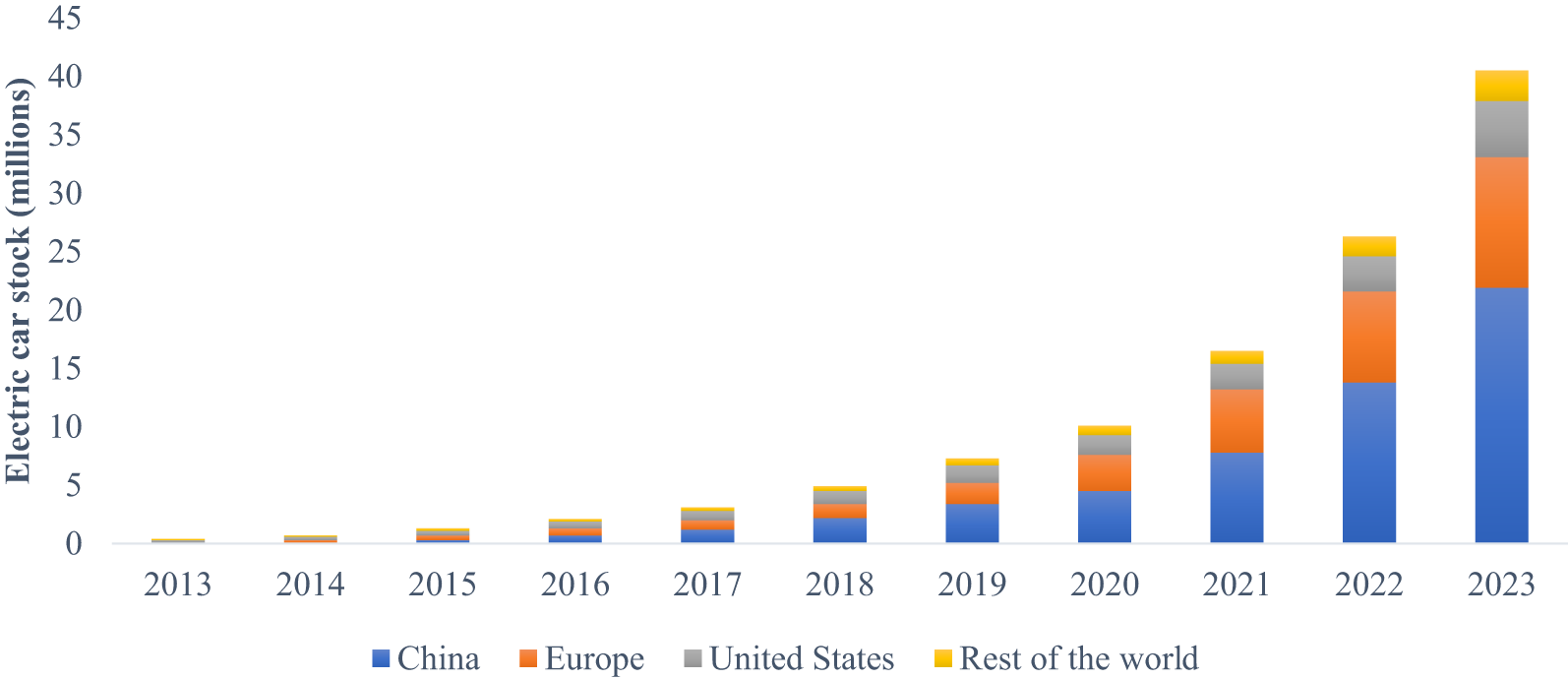
Figure 1: Global electric vehicle stock, 2013–2023 [10]
Different definitions are applied for electric motors, depending on their stage of electrification. The hybrid electric vehicle (HEV) integrates a combustion engine together with an electric-powered thrust device to enhance the overall effectiveness. The plug-in hybrid electric vehicle (PHEV) can use a battery as the main energy source, although the combustion engine supplies reserve power every time the battery loses power. PHEV can be recharged through a connection to the power grid. The battery electric vehicle (BEV) gets its power from the onboard battery and does not use an internal combustion engine, depending on the power grid. In this work, the abbreviation “EV” is applied to any type of car that may be linked to the grid for its recharge or for supplying additional offerings to the grid. Several models of EVs are already combined into the vehicle market. Automakers are introducing more EVs to their product lines. Major automakers have launched various HEV, PHEV, and EV models in the automotive market. It is essential to identify the potential negative effects on the power grids and strategies to overcome the effects of the grid using the ecological and economic advantages of EVs.
New problems arise in the operation and design of electricity systems due to an open market environment and the restructuring of industries in different distribution, generation, and transmission units. In the current energy scenario, utility companies assign more importance to the distribution of safe, controlled, and reliable electrical energy, and electricity networks are divided into generation and transmission networks [11,12]. Power system stability is the capacity to maintain operational balance [13], but this system is affected by varying degrees of frequency fluctuations caused by weak links in the multi-area network. These fluctuations usually continue and grow, and eventually lead to system instability [13]. The power system becomes prone to instability, so fast and high gains are widely used to mitigate these effects due to disturbances, such as sudden load changes, power outages, or switching of transmission lines during faults. Traditionally, stability was generally divided into angle and tension stability. Angular stability can be classified into weak signal stability, transient stability, mid-term stability, and long-term stability. The stability of the system depends on the damping and time components of the torque. Lack of sufficient synchronous torque can cause temporary instability. The high-speed excitation model in modern propulsion systems improves transient stability through damping torque, which makes it a basic and necessary condition to study the stability of weak signals.
The Power System Stabilizers (PSS) were mainly designed for the stability analysis of small signals using techniques for phase compensation, and the PSS parameters were optimized according to the detailed power grid model, including the grid equations [14,15]. Classical PSS-based optimization techniques can provide optimal performance under standard conditions of operation and normal system parameters. In the case of complex and dynamic modern energy systems, the resolution of the problem of low-frequency vibrations using conventional and linear optimal control approaches presents high complexity. The PSS parameters must be adapted for different load conditions and network configurations.
The majority of the transmission lines in a power system are AC, and converter control is needed to regulate them since power flows in AC lines are uncontrolled [16]. Several innovations in the development of electronic switches required for the stability and control mechanisms in the power system have been developed in recent years. These devices are commonly identified as Flexible AC Transmission System (FACTS) [17]. The devices of the FACTS series are designed to increase the stability and resilience of the transmission network, while the FACTS bypass devices are applied to control the bus voltage at the desired value. FACTS controllers have an important contribution to improving network stability due to their fast control behaviour and continuous compensation capability. FACTS devices have been used effectively to accomplish several objectives, e.g., load flow control, loop power flow control, load distribution, voltage regulation, and reduction of system jitter [18,19]. Power deviation of the connection line, deviation of the rotor speed, and shutdown of the generation are exposed under different load conditions. They are broadly categorized as:
1. Series FACTS devices:
a. Thyristor-controlled series capacitor (TCSC)
b. Static synchronous series compensator (SSSC)
2. Shunt FACTS devices:
a. Static VAR Compensator (SVC)
b. Static synchronous compensator
3. Combined series—shunt FACTS devices:
a. Unified Power Flow Controller (UPFC)
b. Inter–line power flow controller (IPFC).
The UPFC combines a shunt-connected device and an SSSC. Several authors have applied UPFCs using different control methodologies, making it one of the most flexible and applied FACTS devices due to increments of dynamic stability and high reliability in active and reactive power control. According to Bindal [20], UPFC is the most versatile and reliable method for dynamic and transient stability, load flow, and voltage control.
The integration of EVs further complicates the grid’s dynamics, particularly in modern AC/DC hybrid distribution systems [21,22]. Recent studies, such as those on the optimal dispatching of AC/DC hybrid active distribution systems [23], highlight the critical need for coordinated control strategies to manage power flow and maintain stability under the fluctuating demand from distributed resources like EVs. The control strategy proposed in this work, combining UPFC and LQR, aligns with this need for advanced coordination in hybrid network environments [24]. Furthermore, the role of EVs extends beyond mere loads to potential grid-support assets; their aggregation and interaction with energy storage can be leveraged for congestion management and enhancing grid resilience [25]. However, this increased digitization and control also introduce vulnerabilities. The resilience of cyber-physical power systems against data integrity attacks, especially on critical control loops involving devices like UPFCs and measurements from Phasor Measurement Units (PMUs), is paramount. While our current study focuses on the fundamental stability improvement using a centralized optimal controller, these aspects of resilience and cybersecurity form a critical foundation for the practical deployment and future evolution of such control schemes in next-generation power systems [26].
Several research studies are focused on the development of a new technique to address relevant control problems in power systems, mainly based on Sliding Mode Control (SMC), proportional-integral-derivative (PID) control, adaptive control, Machine Learning (ML) algorithms, among others. A PID controller is easy to implement with reduced operational costs, but it provides inaccurate performance in anomalous working environments due to its elevated sensitivity. Novel optimization methods have been implemented on PID controllers to enhance the determination of constraints. Other controllers have been proposed with higher stability and reliability. Model predictive control (MPC) is a generic and conventional controller formed by a comprehensive range of control tools. MPC has been widely implemented in multivariable systems to control frequency deviations in traditional and renewable power grids, mainly in multi-area power grids, because this controller ensures high stability in disturbed systems, easy implementation, and fast response [27,28]. One of the most relevant MPC approaches is based on open-loop nominal with constraints, but this approach is too conservative in the development of offline open-loop estimation of the maximum potential perturbation of the disturbance required to calculate the constraints of the model. MPC has been combined with LQR to enhance the frequency stabilization of power grids [29]. It is demonstrated that the reliability of MPC is highly dependent on optimization techniques, and methodologies, strategies, and novel algorithms in MPC are required. A nonlinear MPC (NMPC) is combined with a Sliding Mode controller (SMC) to compensate for this effect and improve the stability and robustness of the methodology. SMC is one of the most effective controllers in PSS for nonlinear control systems because it does not need system parameters for accurate modelling, presenting low sensitivity to variations in plant parameters [30,31]. Yin et al. [32] developed a novel adaptive SMC to increase the strength of the methods, and the results are compared to traditional SMC, obtaining significant improvements. Sebaaly et al. [33] combined SMC with Support Vector Machine to increase performance, robustness, and stability to perturbations in power grids. It is concluded that this controller presents discontinuities with state variables with a determined frequency caused by unmodeled dynamics, leading to losses in control accuracy.
ML algorithms have acquired relevance in the management of energy systems, with Artificial Neural Network (ANN) being one of the most significant techniques. A feed-forward ANN formed by a hidden layer was designed by Shamsollahi and Malik [34] to develop predictive PSS. However, the authors applied a simplified structure to minimize the complexity of the model, as the effectiveness of the controller is affected by several operating conditions that reduce its reliability. Sharma et al. [35] proposed an ANN and the results are compared to PID and Particle Swarm Optimization. The layered recurrent ANN applied two networks to identify specific patterns through the development of training, and it presented better results for all the models considered in this research. The authors demonstrated that the training is the most critical phase, and it is affected by training data, demonstrating that this technique demands high computational costs and advanced training. It requires large datasets to ensure robust controllers, and it is proposed that the application of other ML techniques can solve the weaknesses of this technique.
The novelties of this paper are summarized as:
• Comprehensive Co-modelling: This study presents a comprehensive integrated model that combines the dynamics of a synchronous generator, a detailed two-stage EV fast charger (including its AC-DC and DC-DC converters with associated controllers, and a battery model), and a Unified Power Flow Controller (UPFC). This level of detail in co-simulating these distinct components for small-signal stability analysis is a key contribution.
• Stability Analysis of EV Charging Impact: While previous research has often simplified EV loads as constant power/current loads, this work rigorously analyzes the impact of the voltage-dependent charging behavior of a detailed EV model on the system’s small-signal stability, demonstrating its significant influence.
• Coordinated Optimal Control: The paper proposes and validates a coordinated control strategy where an LQR-based controller is designed for a power system equipped with both a UPFC and an EV load. The results demonstrate that this optimal control strategy effectively mitigates the negative damping introduced by the EV load, outperforming systems with only a conventional Power System Stabilizer (PSS).”
• The analysis of the current state of the art demonstrates that several studies are focused on traditional controllers, e.g., PID and MPC. However, few studies have analyzed and modelled the LQR controllers. These controllers are unfeasible for current technical requirements due to several restrictions and limitations for the overall stability.
• The researchers examined the stability of the power grid with EV with the influence of SVC and TCSC, being one of the most relevant novelties proposed by this study. The test system chosen for the stability study in this dissertation is the Single Machine Infinite Bus (SMIB) system. The system modelling technique shown in this work can be implemented in a more complicated and larger multi-area system for better and more practical analysis.
2 Stability of Small Signals of SMIB
This section is focused on the stability of small signals of the SMIB system. The low-frequency oscillations (LFO) are examined due to the load changes in the power system. These frequency oscillations can lead the system to instability if appropriate damping is not provided. These oscillations can be classified according to their type of connection in the form of local modes; inter-area modes; and tortional modes. In this section, the influence of PSS on the SMIB system in the case of LFO is also examined.
2.1 SMIB: Small Signal Stability
The SMIB model is studied in the Heffron-Phillips model and applied by Demello and Concordia to analyze small signals. The flux decay system is linearized using Ed (EMF caused by the d-axis of the generator) in this model, being introduced as a fast-acting exciter. Certain constants (k1 to k6) are defined in this state space model, being functions of the operating state. The state-space model is implemented to test the eigenvalues and design additional controllers to obtain sufficient damping. The electromechanical model presents real and imaginary components that are associated with damping and synchronization torque [36,37].
ω0 = synchronous speed (rad/sec)
ω = alternator steady state angular speed (rad/sec)
δ = angle of induced voltage (v) (rad or degree)
Vd = direct axis component of the phase voltage at the terminal in (p.u)
Vq = quadrature axis component of phase voltage at the terminal in (p.u)
V = terminal voltage per phase in (p.u)
Ed’ = direct axis component of stator induced emf (p.u)
Eq’ = quadrature axis component of stator induced emf (p.u)
E’ = stator induced emf per phase (p.u)
Id = direct axis component of armature current (p.u)
Iq = quadrature axis component of armature current (p.u)
Efd = open circuit terminal voltage per phase (p.u)
Xd = direct axis synchronous reactance (p.u)
Xq = quadrature axis synchronous reactance (p.u)
Xd’ = direct axis transient reactance
Xq’ = quadrature axis transient reactance (p.u)
H = inertia constant (seconds).
The simplified SMIB is shown in Fig. 2. Let us consider that a synchronous machine is associated with the bus with an impedance (Zl = Rl + j Xl).
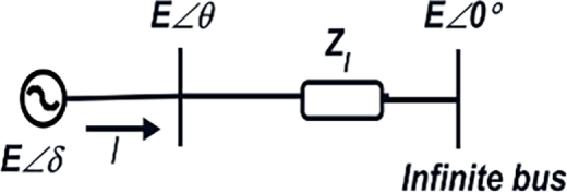
Figure 2: Diagram of simplified SMIB model
Differential equations of the flux-decay model are defined as:
The stator algebraic equations are:
And
Let us consider Rs = 0 for this model. Therefore, Eqs. (4) and (5) can thus be rewritten as
Now
Hence,
Expanding the RHS
Equating the real and imaginary parts,
Substituting of
Cross multiplication and separation into imaginary parts yield
Therefore, the differential equations are represented by Eqs. (1)–(3), and algebraic equations are provided by Eqs. (8)–(11) for an SMIB model.
Now, let us linearize these Eqs. (1), (2) and (8)–(11) around variables Id, Iq, θ, Vd, and Vq.
It is defined as:
Eqs. (13) and (14) are obtained with the linearization of the three differential Eqs. (1)–(3) and replacing the values of Id, and Iq:
Substituting for d
A simplified fast-acting static exciter is now considered, being described with a first-order block with a gain Ka and time constant Ta, as shown in Fig. 3.
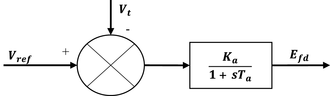
Figure 3: A fast acting exciter
The exciter equation is observed in (15):
Except for k3, which is the impedance ratio, all parameters (k1 to k2) vary according to operating conditions. These equations represent the linearization coefficients for small disturbances of a single generator related to an infinite bus through an external impedance. The suffix 0 represents the initial value. The linearized Philips-Heffron model is shown in Fig. 4.
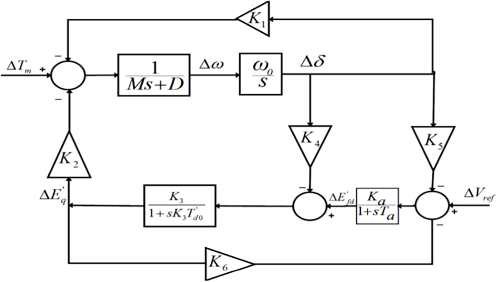
Figure 4: The linearized Philips-Heffron model
An approach to resolve the problem of unstable oscillations generated by the power system is to provide supplementary damping (for the rotor winding) to the generator rotor. It can be performed by traditional PSS, providing drivers for the excitation system [38]. The Vs input of the exciter, see Fig. 5, is the output of the power regulator, and its input signal depends on the speed (or frequency) of the rotor. The traditional drive stabilizer is modelled as follows: PSS is composed of three blocks.
• Washout Gain
• Washout Circuit
• Lead-Lag Compensator
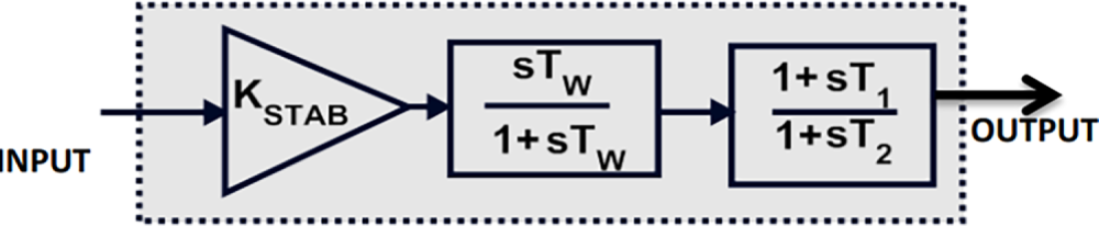
Figure 5: Conventional PSS
The gain of PSS shows the amount of damping, i.e., increases in the gain improve the act of damping. This gain Kpss can range from 20 to 200.
This washout circuit is a high-pass filter that ensures that the PSS only reacts to the generator’s speed deviations and avoids a reaction to the stationary condition of the system. This Tw can be chosen from 1 to 10 s.
This block has a lead-lag compensator, as it is observed in Fig. 4. The number of lead-lag compensations is dependent on the total phase lag of AVR and the field of the generator, although each stage of the compensators, T1, must be greater than T2 to give the lead phase.
2.3 Linear Quadratic Regulator (LQR)
The linear-quadratic controller is a classic optimal state feedback controller that reduces deviations in the state paths of a system with minimal control effort [39]. The objective of the Linear Quadratic Regulator (LQR) controller is to maintain optimum system performance by reducing the cost function between the control input vector and the state vector. Using the Lyapunov method, the LQR design problem of the algebraic equation is explained by the algebraic Riccati equation (ARE) that provides the transformation matrix P between main and secondary states. The optimal state feedback gain is used by the ARE solution in the optimization technique based on the Lagrange multiplier. The weighting matrices LQR regulate the disadvantages for deflections in the paths of the state variables x and the control input u. If the matrices Q and R are selected randomly, the optimal controller does not provide a significant amount of point tracking performance, caused by the lack of an i-term integral as opposed to PID controllers. For this reason, the main issue in designing an optimal controller with LQR is the selection of Q-matrices and R Conventional. The matrices Q and R are adjusted to get the required value iteratively, following the experience of the developers. Any values of Q and R may lead to variations in the system reaction, indicating that the reaction is not optimal. A systematic approach is defined for the choice of the weighting matrices to determine the original values of the Q and R matrices. However, this methodology only proposes initial values and then iterates the coefficients to obtain an optimal Le, which will be adjusted accordingly. The second-order crane system was presented in reference [40], while the concept of a third-order magnetic levitation system is extended in this paper, proposing a systematic framework for the selection of weighting LQR matrices. The advantages of the methodology provide a methodical approach to the selection of the weighting matrices based on the design guidelines, reducing the time of the optimal state feedback controller by using basic mathematical equations to select the Q and R matrices, which significantly reduces performance. The objectives of time-domain systems in cost conversion allow a simple and modular LQR design.
The following subsection details the step-by-step formulation of the LQR controller, including the state-space representation, cost function definition, and the procedure for obtaining the optimal feedback gain.
2.3.1 Design of LQR Controller
It is determined that the role of LQR is to provide the controlled input vector u(t) to achieve the minimization of the performance index J:
The matrices Q and R establish the relative significance of the error and the consumption of this energy. Eq. (16) can be rewritten as (17)
The equation is determined as given in (18) to solve the parameter-optimization problem
Using both sides of (19), it is obtained that this equation must be valid for any x,
It is known that R is a positive Hermitian, so it is possible to write (R = TTT), where T is a non-singular matrix and:
The minimization of (17) is required to obtain the minimization of J concerning K:
From (22), it is possible to obtain (23) and (24)
Thus, a control law is defined by Eq. (25)
in which P must satisfy ARE (26)
Step 1: Collect data for Matrix A, B, Q, R and N. These are the primary variables necessary to model LQR. Generally, both Q and R are positive real symmetric matrices, and the d value of matrix N is zero.
Step 2: Calculate Eigenvalues ‘e’, P matrix using Eq. (26), and K matrix using Eq. (24) above.
These steps can be simplified by MATLAB command [k, p, e] = lqr(A, B, Q, R).
The performance of the SMIB system is established by using software called MATLAB/SIMULINK.
The SMIB system parameters without PSS:
Generator:
Excitation system:
Transmission line:
PSS parameters:
Table 1 shows the system parameters for SMIB with PSS/LQR analysis.
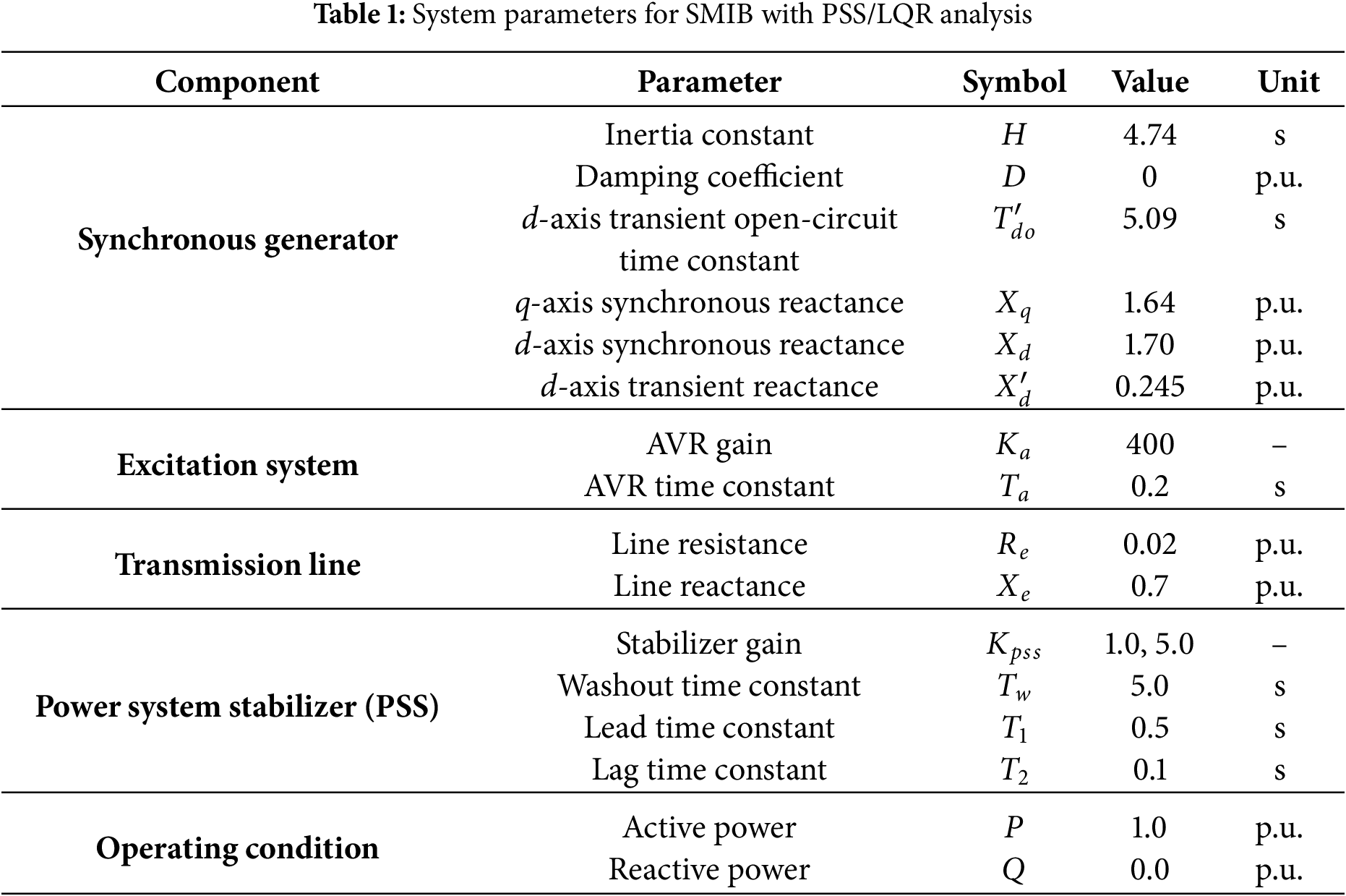
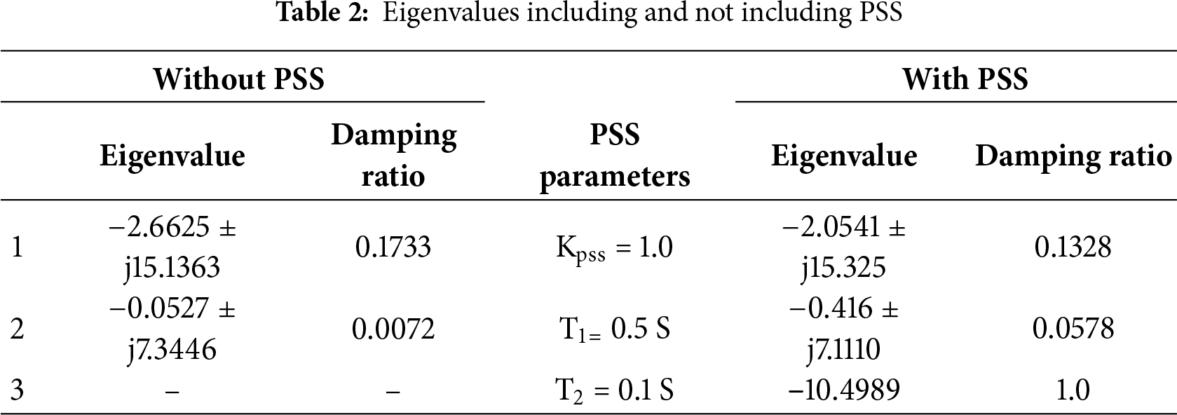
Using the above operating conditions, the eigenvalues and the electromechanical swing modes of a SMIB system are computed from the system matrix. The eigenvalues and damping ratios are given in Table 2 with and without PSS.
Case 1:
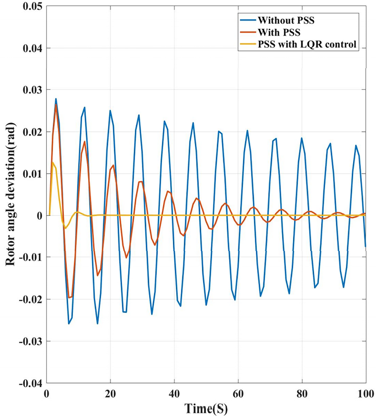
Figure 6: Rotor angle deviation of the system without PSS, with PSS, and PSS with LQR control
Case 2:
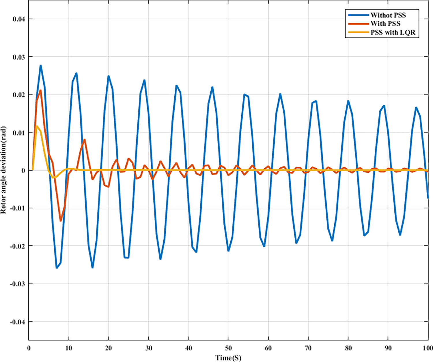
Figure 7: Rotor angle deviation without PSS, with PSS, and PSS with LQR control
It is observed from Figs. 6 and 7 that PSS with LQR control in the SMIB system gives a better response.
System eigenvalues and damping ratios of the electromechanical mode are observed in Table 3 when subjected to different operating conditions.
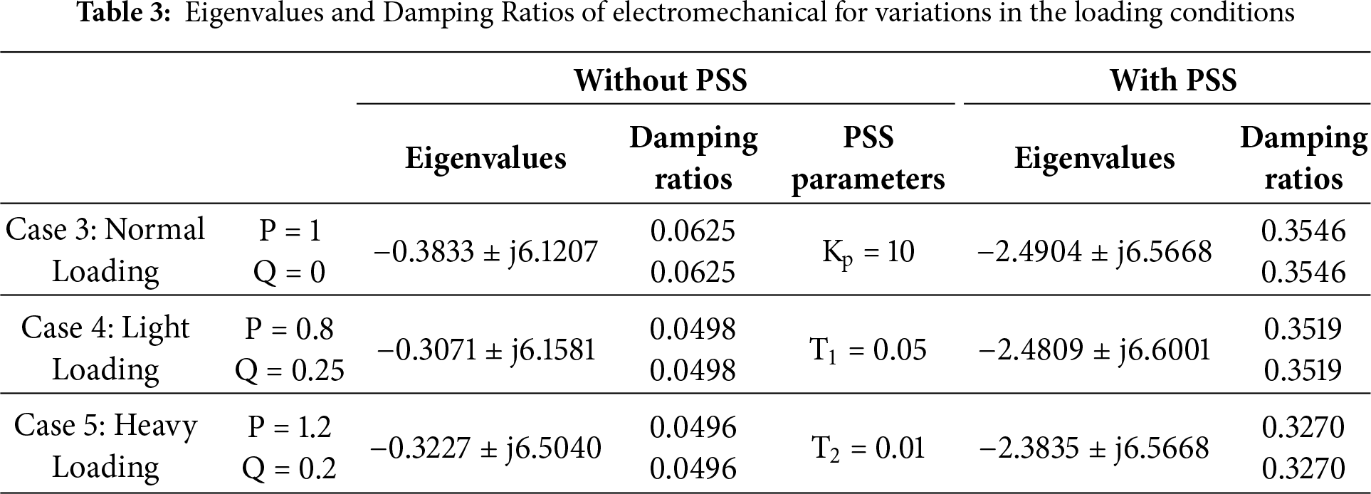
The deviation of rotor angle and rotor speed is observed in Fig. 8a,b, respectively.
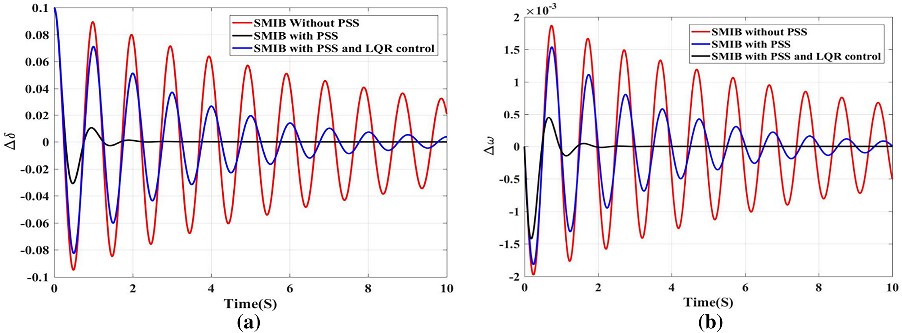
Figure 8: (a) Deviation of the rotor angle for normal loading conditions. (b) Deviation of rotor speed for normal loading conditions
It has been demonstrated that in all the cases, normal loading conditions with properly tuned PSS and LQR provide better damping to the system.
3 Modelling with Unified Power Flow Controller
Different LFO between 0.1 to 3 Hz are examined when large power grids are associated using weak links. These oscillations can continue and grow, and if the damping is insufficient, they will cause the separation of the system [41]. Over the years, by applying additional stabilization signals to the voltage reference input of the automatic voltage regulator (AVR), the installation of a PSS offers a simple and cost-effective way to generate damping torque values, thereby improving the performance of the system stability. However, when the operating conditions of the system change significantly, its performance will decrease [42,43]. It is therefore necessary to apply new management strategies in emergencies, such as failure of power lines and/or generators to operate the energy system effectively without compromising system safety and energy quality. FACTS is an efficient methodology that has emerged as an effective approach to control power flow and suppress network fluctuations. Although the damping coefficient of FACTS-based stabilizer controllers is usually not their leading application, their capability to improve the damping performance of the drive system has been recognized [44,45]. Fig. 9 shows a schematic of the overall study system showing the SMIB, UPFC, EV load, and the LQR control loop. The UPFC is one of the most relevant FACTS product series, and its main objective is the control and optimization of the flow of active and reactive power, voltage, and current of a certain line on the UPFC bus, see Fig. 10 [17]. This is performed by adjusting the monitoring variables of the transmission system, e.g., voltage, impedance of the line, and phase angle [39]. In addition to these basic functions, it can also ensure an effective damping effect through an additional controller to limit the oscillation of the electrical system of the networked modern automobile and increase the system stability [46].
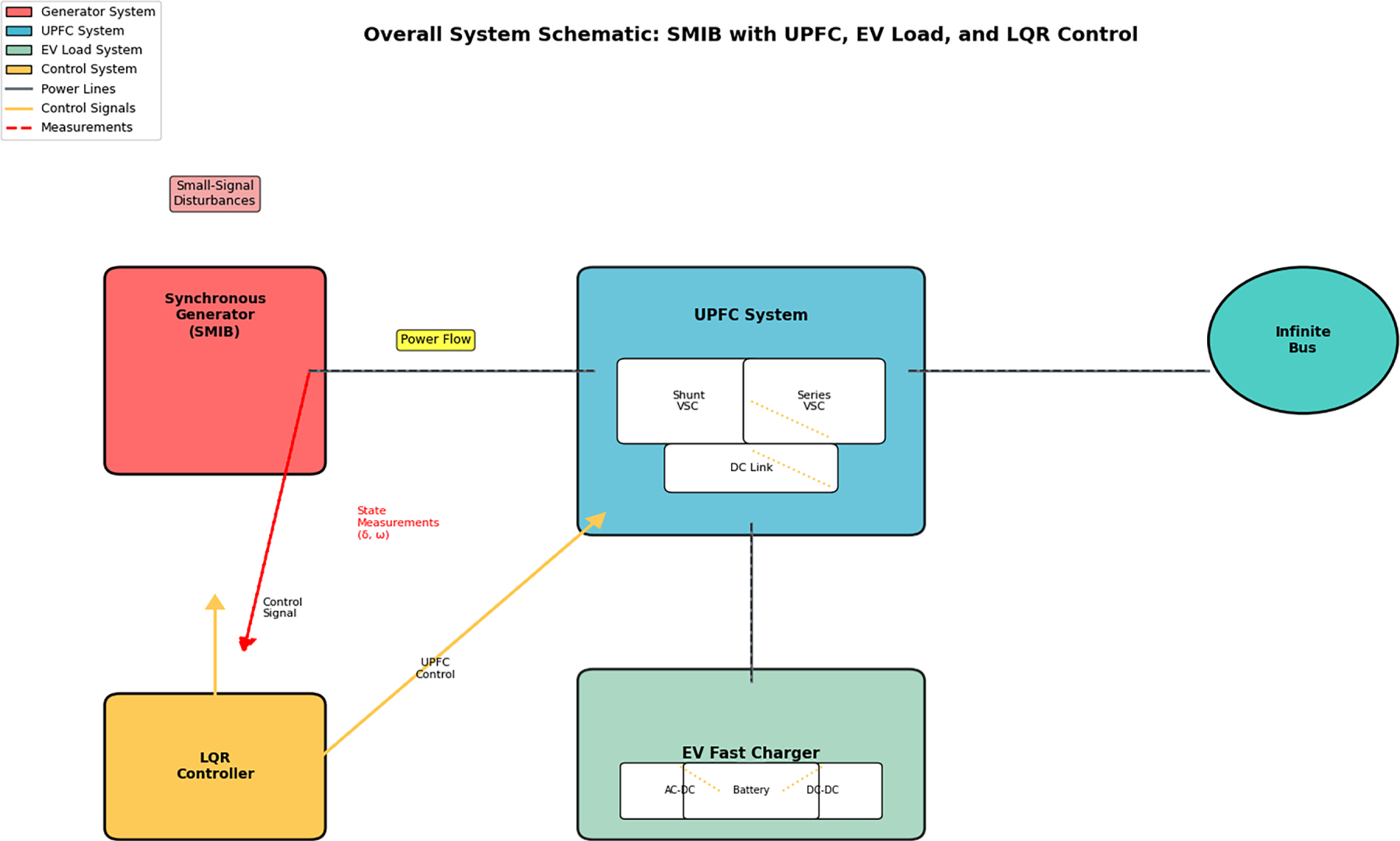
Figure 9: Schematic of the overall study system showing the SMIB, UPFC, EV load, and the LQR control loop
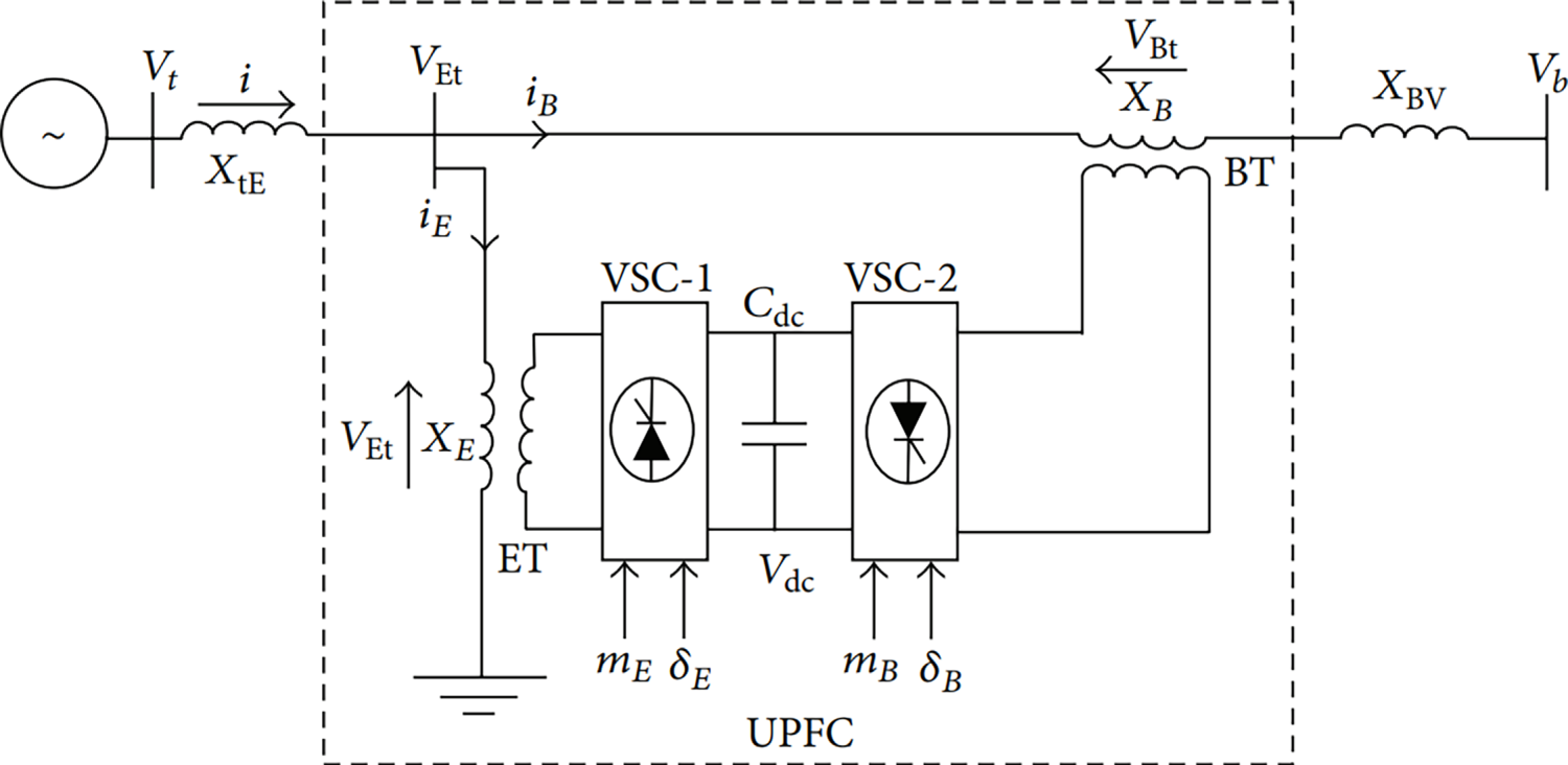
Figure 10: SMIB system with UPFC
It is considered that the possible connections between the PSS and FACTS damping controllers can enhance the overall performance of the electrical system, but the inconsistent local design of the PSS and FACT damping controllers can lead to unstable interactions when the damping system vibrates [47]. The synchronized design of stabilizers based on PSS and FACTS is necessary to use multiple stabilizers to improve system stability and avoid inconveniences related to their operation.
The test system used for this study is a standard Single Machine Infinite Bus (SMIB) system, a well-established benchmark for small-signal stability analysis.
3.2 SMIB Model Equipped with UPFC
The SMIB installed with UPFC, see Fig. 11, and the SMIB with UPFC with DC voltage, see Fig. 12, both with a power oscillation damper (POD) in the input state. The generator drives numerous buses through transmission lines and UPFC. The UPFC is formed by two GTO-based three-phase VSCs, which are fully coupled with a common DC link. VSC-1 is connected in shunt with the line through an excitation transformer (ET), while mE and δE variables characterize the amplitude modulation ratio and phase angle signals. The parameters mB and δB signify the amplitude modulation ratio and segment perspective alerts of converter VSC-2, which is introduced in series with the transmission line by a boosting transformer (BT). Synchronized energy compensation in sequence line with the external voltage supply is provided by these four input control inputs of UPFC.
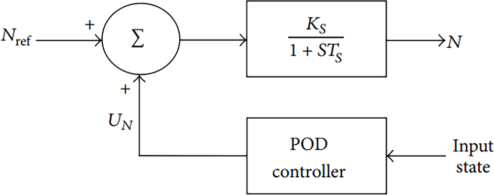
Figure 11: UPFC with damping controller
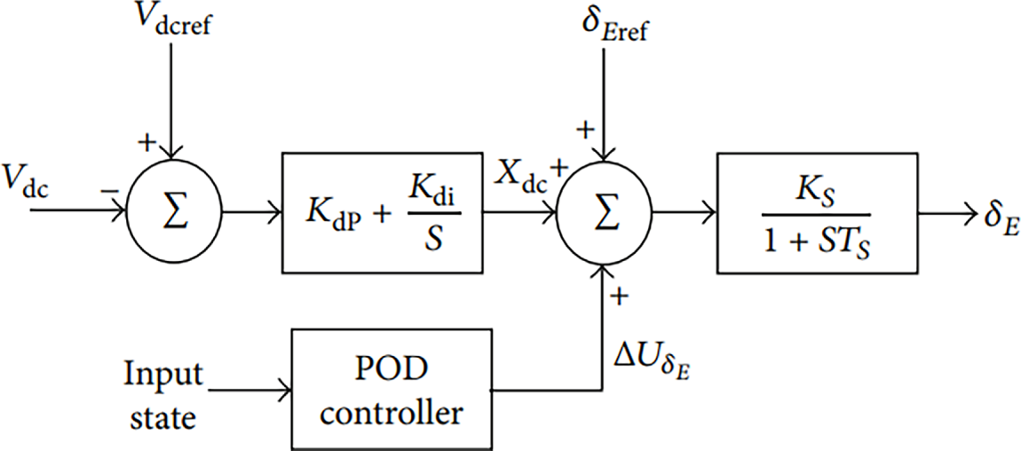
Figure 12: UPFC with damping controller and DC voltage regulator
Considering Fig. 11, it is determined that:
VEt = excitation transformer voltage
iE = excitation transformer current
rE = excitation transformer resistance and lE = excitation transformer inductance.
Similarly,
VBt = boosting transformer voltage
iB = boosting transformer current
rB = boosting transformer resistance and lB = boosting transformer inductance.
For this case, it is not considered the resistance and transient of UPFC transformers, and applying Park’s transformation it is obtained the following equations are obtained:
where XE = ET reactance and XB = BT reactance.
From Fig. 10, it is provided:
where Vt is the voltage of the generator terminal, Vb is the infinite-bus voltage, xtE and xBV are the transmission line reactance, and I is the armature current. Now, the armature current and terminal voltage can be written considering the d-axis and q-axis components:
Now, from Eqs. (33) and (35), it is provided the following equations:
Again from (36)–(38), we can have the current injection of UPFC as:
where,
3.4 Linearized Model of SMIB with UPFC
Using the SMIB model defined in the previous section and the UPFC model defined in Section 3.3 around the nominal operating conditions, it is defined as:
where,
being the linearization constants K1–K9, Kpc, Kpe, Kpδe, Kpb, Kpδb, Kqc, Kqe, Kqδe, Kqb, Kqδb, KVc, KVe, KVδe, KVb, KVδb, Kce, Kcδe, Kcb, and Kcδb the initial operating conditions and the functions of the system parameters.
Representing these equations in a state space model as:
where,
and
The Phillips-Heffron including UPFC transfer function model presents 28 constants, while the Phillips-Heffron model includes only 6 coefficients, as observed in Fig. 13, demonstrating that the damping torque is given by the UPFC. UPFC is separated into two parts: direct-damping torque and different coefficients. The direct-damping torque is used in the electromechanical oscillation loop of the generator, whose sensitivity is mostly quantified by the constants Kpc, Kpe, Kpδe, Kpb, and Kpδb. The second part is formed by the coefficients KVc, KVe, KVδe, KVb, and KVδb being applied for the generator field channel. Its sensitivity is attached to the field voltage deviation, described as the indirect-damping torque.
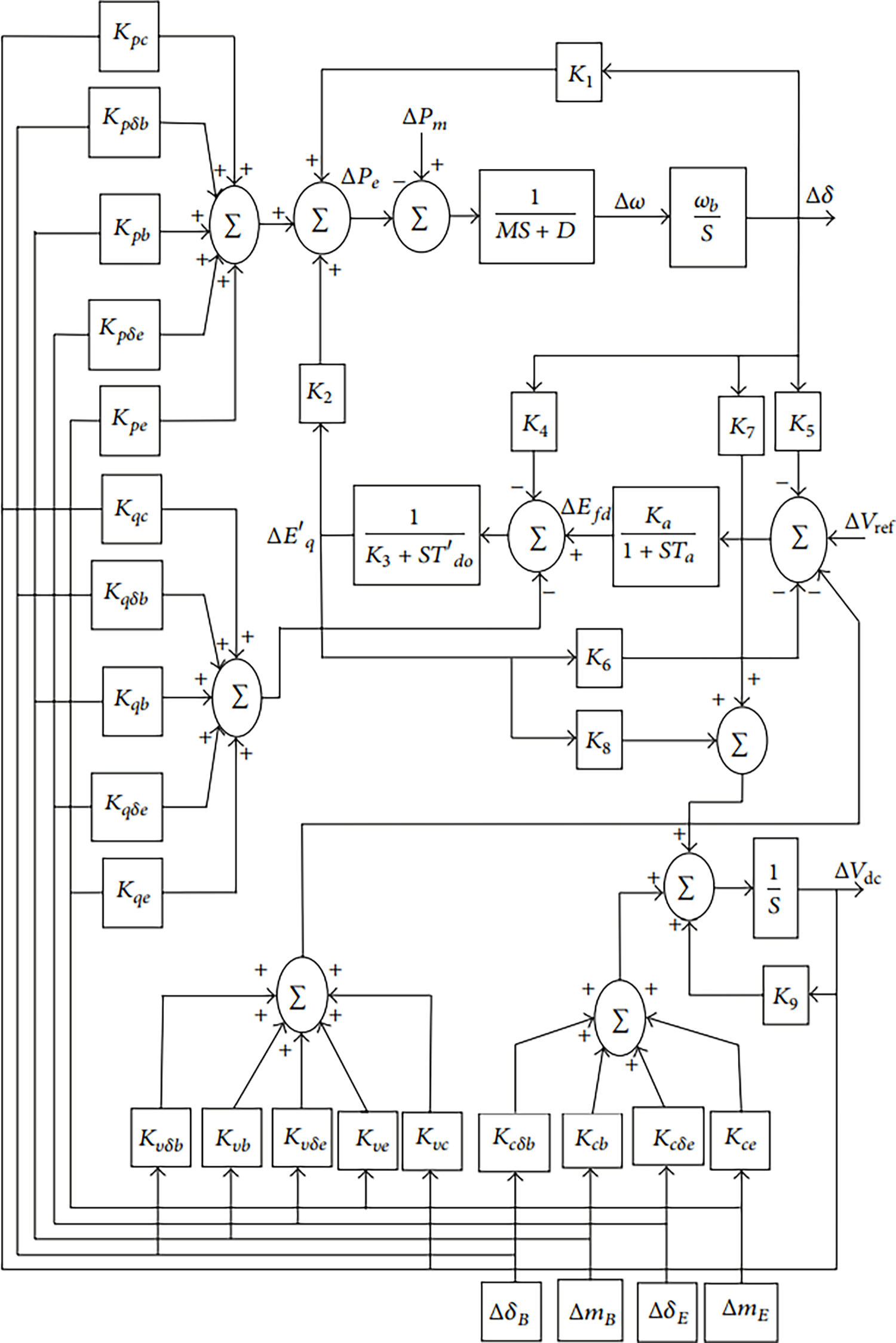
Figure 13: Adapted Heffron-Philips transfer function model of SMIB power system with UPFC
The performance of the SMIB with the UPFC system is developed by applying software called MATLAB/SIMULINK. The SMIB system parameters without PSS:
Generator:
Excitation system:
Transformer:
Transmission line:
Operating conditions:
UPFC parameters:
Table 4 shows the system parameters for SMIB with UPFC Analysis
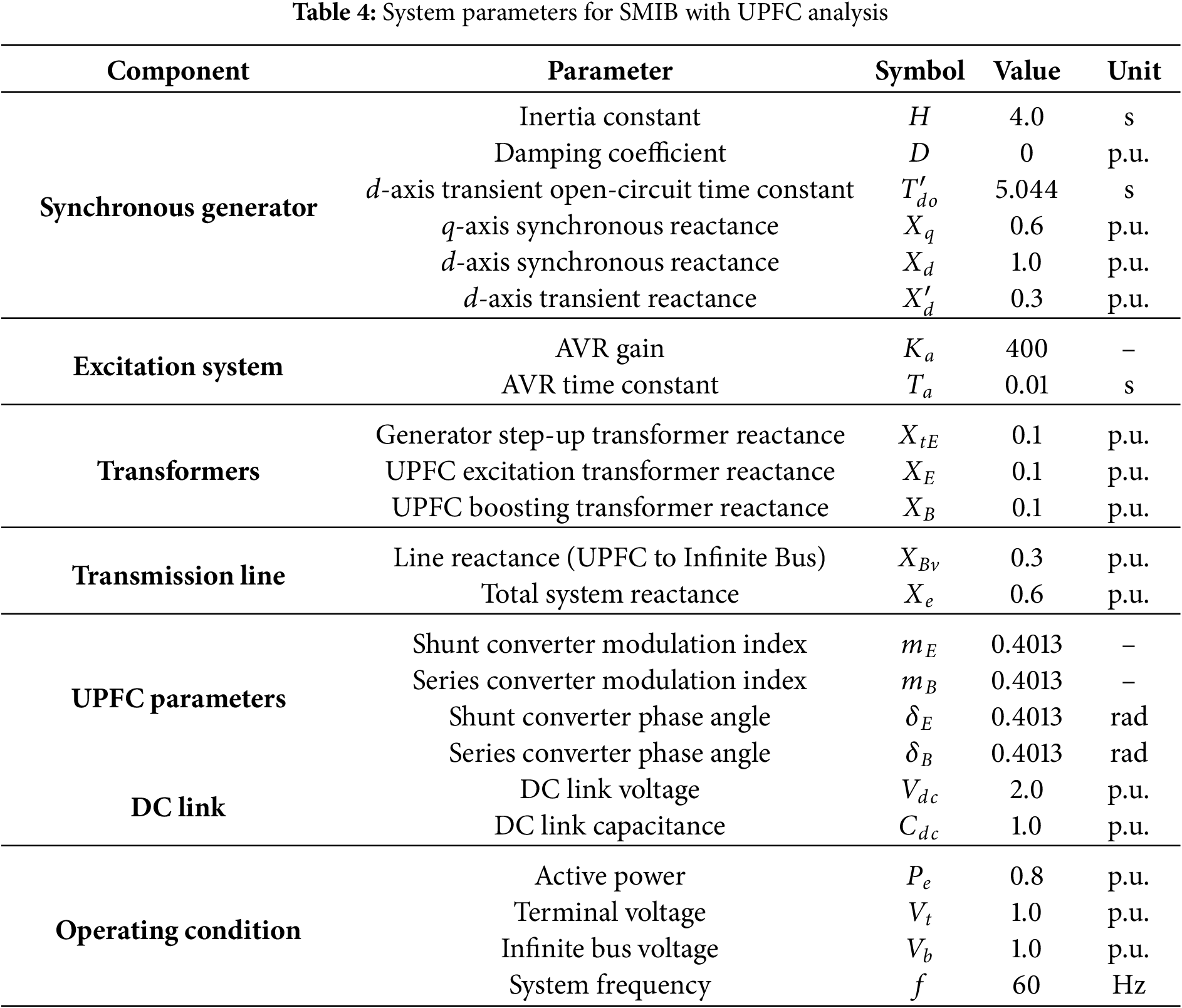
Parameters of DC link:
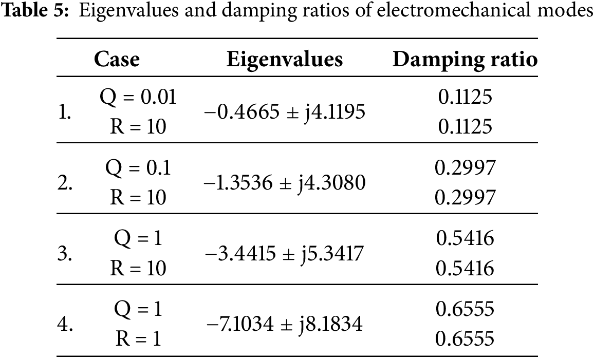
The eigenvalues and the Damping ratios for different cases are computed in Table 5.
The deviation in rotor speed and angle is shown in Figs. 14 and 15, respectively.
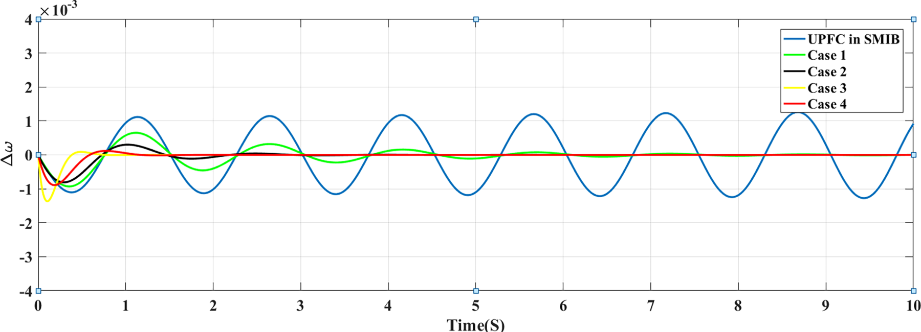
Figure 14: Deviation in rotor speed in SMIB with UPFC and UPFC with LQR control
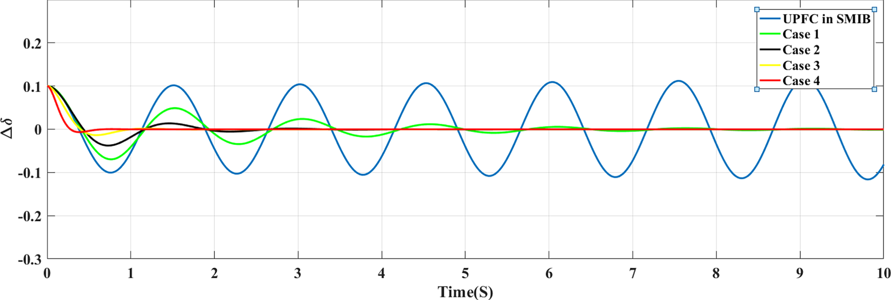
Figure 15: Deviation in rotor angle in SMIB with UPFC and UPFC with LQR control
Table 5 shows the eigenvalues and damping ratios of the electromechanical mode using different weights of Q and R matrices. The parameters Q and R applied for this study for Figs. 14 and 15 are parameters designed to apply penalties for state variables and control signals. It is observed from the table that the higher these values are, the higher penalties are applied to these signals. It is established that larger values for R involve more stabilization of the system with reduced weighted energy. Furthermore, the selection of a small R-value implies that it does not pretend to penalize the control signal, being a low-cost control strategy. In the same way, the selection of larger values for Q implies that the stabilization of the system is performed with minimal state changes, while larger Q values involve less concern for the changes in the states. It is confirmed that a suitably tuned LQR gives a better response.
4 Modelling of Electric Vehicle Load for Stability Studies
The incorporation of EV in the power grid poses significant challenges to electrical engineering around the world. Evaluating the potential impact of integrating EVs into the network is critical to the safe operation of the network. Researchers have studied various topics related to the integration of EV networks. However, the literature search in the next section shows that the impact of EV charging on the stability of the power system is not fully understood [48]. The main factors with high influence on the instability of the system are the stability of the voltage and the ability to resist fluctuations. However, an accurate load model of EVs has not been developed to study system stability. Therefore, this section discusses the advancements of static and dynamic charging systems for EVs. EV chargers are mainly divided into AC chargers and DC chargers, depending on their performance and charging status. Tier 1 chargers are mainly used for household charging. The Tier 2 charger can be a household or industrial charger according to its rating, while Tier 3 chargers are fast commercial chargers. The rated output of the fast charger may reach 200 kW [49], reducing the charging cycle to a few minutes. It is comparable to the average refuelling time of a traditional car. Fast charging is likely to become popular because it will be a suitable and efficient charging solution for electric car users. It is essential to evaluate their impact on the energy system. Although there is a charging model derived from experiments for charging equipment for level 1 EVs, there is currently no charging model for fast charging equipment for EVs. Their static and dynamic behavior is shown in this study.
The robustness of the research results on the influence of EVs on the electrical system depends on the accuracy of the simulation, which contains the built-in load model to characterize the EV load. The simulation of the EV load needs to characterize the EV as a function of the power supply voltage. However, various types of charging models have been used in the state of the art to illustrate the charging behavior of EVs in power system research, including EVs that are considered to be constant current charging; on the other hand, EVs are characterized by stable performance. In addition, these links are based on a derived load model rather than a derived model. The ZIP model was used in the study, and model tests were not referenced. In addition, school and room models of EVs have also been developed in, can be used to analyze the demand for EVs. In the estimation of the dynamic model used for the single-stage charger of EVs, the small number symbols proposed in [50] for the probability research of the small signal stability and the stability research are found. However, modern high-performance chargers will significantly affect system stability and are composed of two stages (AC-DC and DC-DC) instead of a basic single-stage structure (AC-DC). It is important to create a system charging model to represent the charging of EVs for accurate studies of stability and reliability. A verified EV charger is formed by two converters, namely the front-end AC-DC converter and the battery-side DC-DC converter, as observed in Fig. 16. This is accomplished by turning on the active rectifier or combining the rectifier with a circuit of power factor correction, as it is defined in [51]. The second phase uses several types of DC/DC converters, with resonance or pulse width modulation (PWM). It is required a DC/DC converter is required to preserve a charging current suitable for various states of charge (SOC) requirements and battery cell temperatures. Therefore, the second stage of the converter keeps the ripple of the charging current within the safe range of the battery.
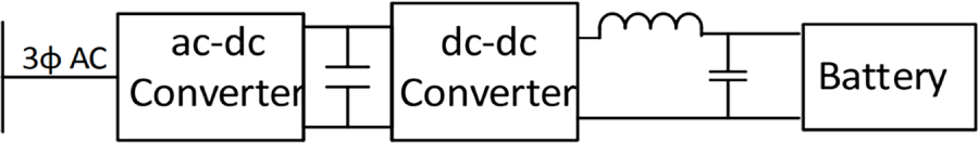
Figure 16: EV charger schematic diagram
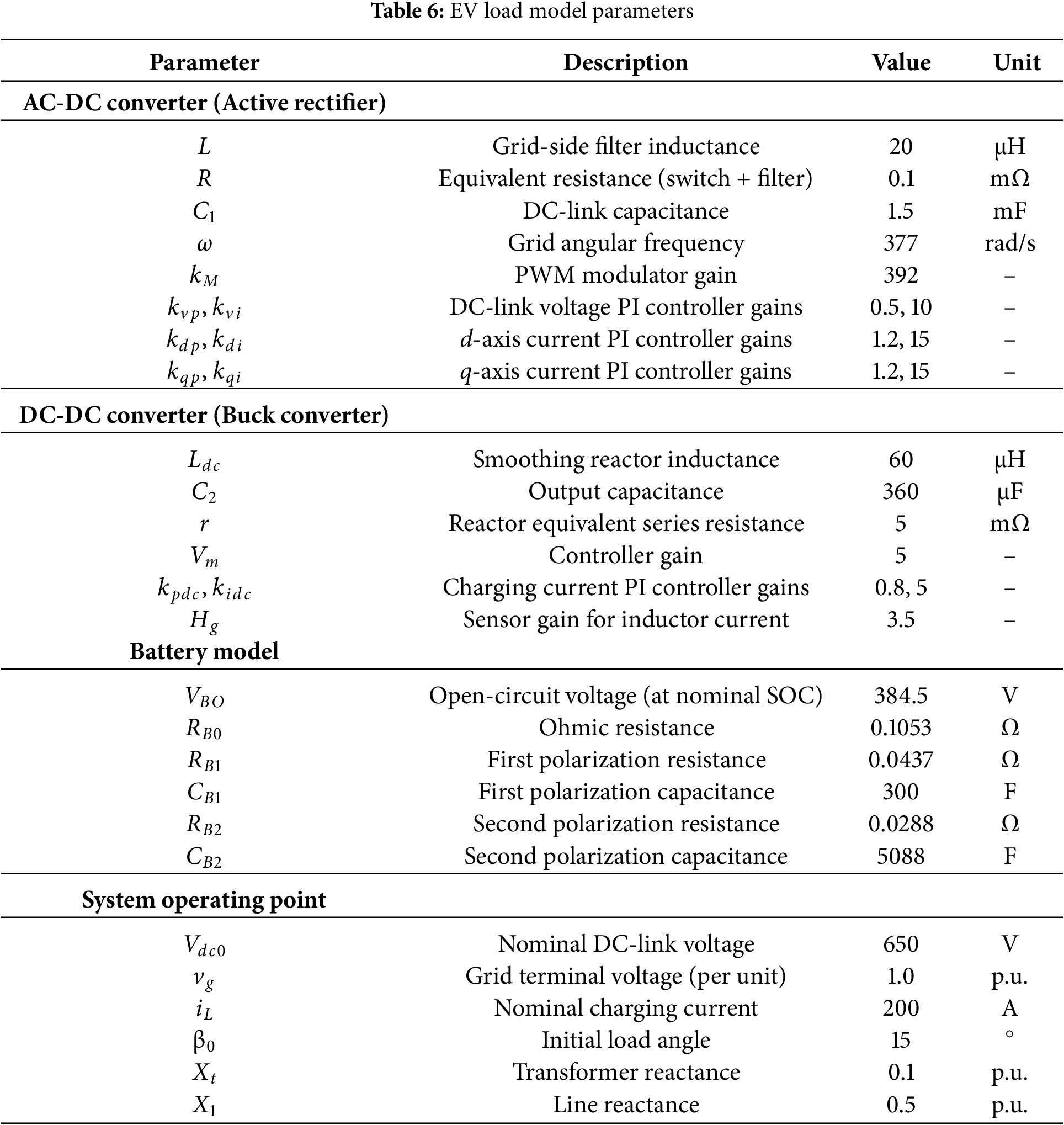
It is considered here a fast charger for EVs, based on an active rectifier front end and a DC/DC step-down converter to simulate the static and dynamic charging behavior of EVs. Table 6 shows the EV load model parameters.
4.2 Static Load Model Development
The static analog DC fast charger presented in this section is formed by an active rectifier and a step-down converter on the battery side. This charging circuit presents several suitable characteristics, e.g., unit power factor operation and the capability to connect to diverse input voltages. It produces a stable DC output voltage that is not affected by input voltage fluctuations within specific limits. In addition, it has emerged as an effective and attractive alternative for medium power applications beyond several kilowatts. The active rectifier can limit all harmonic distortion. The charging configuration is determined in Fig. 17.
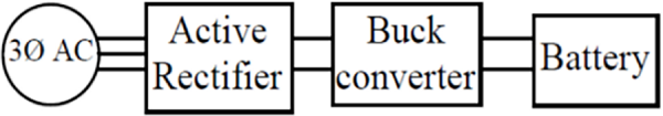
Figure 17: EV fast charger schematic diagram
The load simulation applied to check the voltage reliability of the electrical system needs to regulate the load change compared to the supply voltage. The power-to-voltage ratio is determined through analysis of the charger as displayed in Fig. 18.
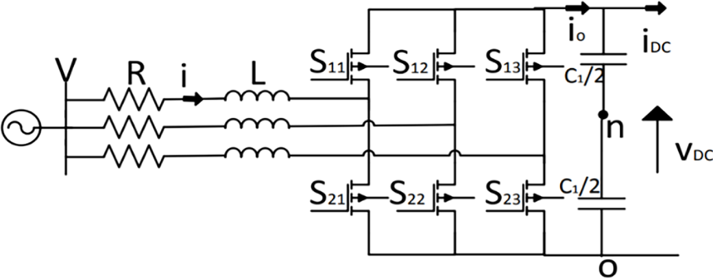
Figure 18: Circuit diagram of an active rectifier connected to the grid
From Fig. 18, the following equations are developed [52]:
The S11, S12, S13 = 1, when the switches are in the ON state; otherwise S11, S12, S13 = 0. R is the impedance of the first stage of the converter. The resistor R consists of the active rectifier switch resistor (Rs) and the parasitic input filter resistor (RL). The inductance of the input filter choke is represented by L. For a symmetrical three-phase system, adding (51) to (53), we get Eq. (54).
Now we can rewrite (51)–(53) as (55)–(57):
The output current io of the active rectifier at any instant is given by (58):
and, it is provided
Representing the above equations in dq reference
where,
with
Now, representing dd and dq in dq reference frame:
Dd and Dq are in an established employment relationship. The active and reactive power in the Dq reference frame are obtained from Formulas (68) and (69).
The AC/DC converter illustrated in Fig. 19 controls the DC link voltage and continues the operation with a power factor of 1. The D-axis current is applied for adjusting the intermediate circuit voltage.
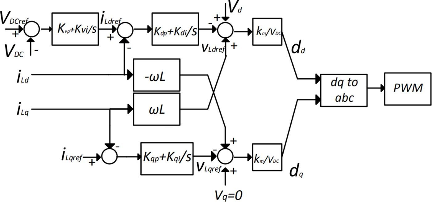
Figure 19: Circuit diagram of active rectifier controller
The dq-frame rotates at a speed ω, and the d-axis is aligned with the voltage vector of the network. Therefore, Vq = 0. In addition, iqref is set to zero to ensure unity power factor operation. Condition, iq = 0. (65)–(68) can be modified in (70)–(73).
Considering (70), (72), and (73),
Now, let us consider the second stage of the EV fast charger, i.e., the buck converter, see Fig. 20.
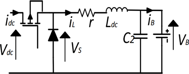
Figure 20: Circuit diagram of the buck converter
From Fig. 20, the following Eqs. (75) and (76) are obtained:
Being VB, the battery terminal voltage is defined by battery characteristics and charging current. It mainly relies on the state of charge of the battery, the impedance, and the charging current. The reference charging current is defined by managing the battery system through the monitoring of battery voltage, temperature, and SOC. The constant current and constant voltage (CC-CV) charging method has been highly used as the main battery charging method. In the first charging phase, the buck converter regulator provides constant values of the charging current. When the battery voltage achieves the set value, a constant derating current is introduced into the battery until it is completely charged. This includes simulated drumming. The battery can be defined as an alternating voltage source (EB), which is related to a series with a resistor (RB1) and a parallel combination of alternating current. The capacitor (C) and resistor (RB2) are determined in Fig. 21.
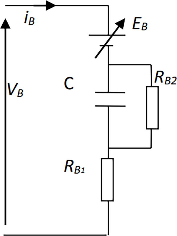
Figure 21: Battery model schematic diagram
The capacitor may be opened for static analysis. Therefore, the resistor (RB = RB1 + RB2) in series with the AC voltage source (EB) is equivalent to a battery. The established views of (75) and (76) are given in (77) and (78).
The buck converter must operate in a lossless switching mode with constant conduction. Considering the steady-state operating mode ratio k, the steady-state equation can be derived from the following equations:
Combining (74), (79), and (80);
Therefore, the power supply voltage depends on (Pvd). This component can be expressed as (49).
This corresponds to the standard exponential charging mode, as shown in (84), which has a negative alpha value, where P0 is the power consumption at the reference voltage (V0).
4.4 Modelling of the AC-DC Converter and Controller
The dynamic model of the AC-DC converter determined in Fig. 17 is derived from here. A dataset of differential and algebraic equations is derived to define the features of the transducer. AC operation is carried out in the dq framework, and the DC-DC boost converter can be defined as follows. The method of converting abc to dq is described in Section 4.3, and more information can be found in reference [53].
By selecting d axis along the grid voltage vector VL∠θ,
The Eqs. (98) and (99) can be rewritten as,
The real and reactive e power consumption are calculated as,
Considering the power balance of the rectifier and accepting lossless switching,
The simulation of the AC-DC converter controller is shown in Fig. 19. It supports operation with one DC link voltage and power factor, as observed in Section 4. The variables x1, x2, and x3 are three added state variables to label the dynamic behavior of the AC-DC converter controller.
Solving (92)–(94) and (95)–(98) we get,
And,
4.5 Modelling of DC-DC Converters and Their Controllers
This section analyses the second stage of the charger, based on a DC-DC converter. This converter and its controller are described in Fig. 22, and they require lossless switching and buck converter control. The battery charging reference current (IBref) is established by the battery management system based on various factors. The effective series resistance of the current smoothing reactor is r, and the proportional constant and PI integral constant are called kpdc and Kidc. The analytical expression of the second stage is as follows: Variable x4 is an aggregated state variable, which describes the DC dynamics of the DC/DC converter regulator.
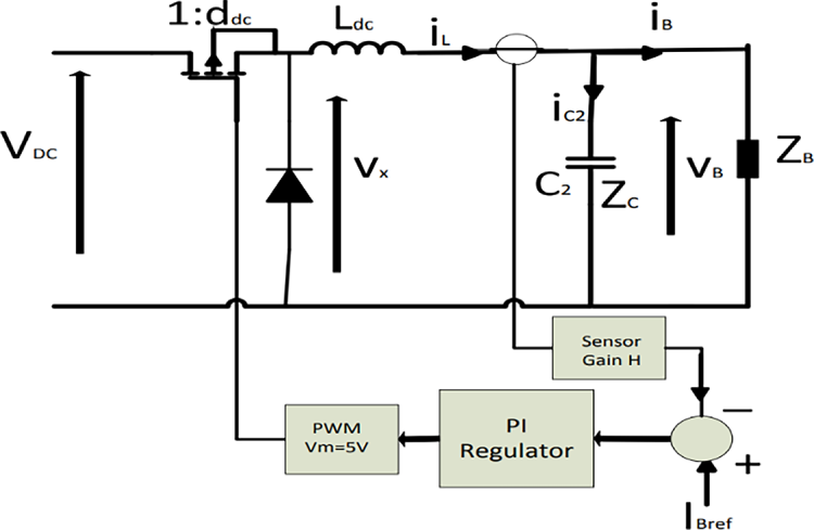
Figure 22: Circuit diagram of DC-DC converter and controller
Modern electrical equipment uses lithium-ion (Li-ion) batteries or nickel metal hydride (NiMH) due to better unit energy and longer service life [21]. The dynamic performance of the Li-ion battery determines that the thermos-electrochemical reaction uses a certain area when charging or discharging the battery. Battery performance depends on SOC, operating temperature, charging or discharging current, supplier availability, etc. Machine simulation used for vibration balance research requires a service factor version determined by the battery, and the complexity of the battery model should be reduced without affecting its accuracy if the motor is hardly disturbed. The thermal battery model defines the effect of changes in electrolytes and ambient temperature on battery performance. Li-ion batteries contain an advanced liquid cooling system, while NiMH batteries use a simple forced air-cooling system, and it can be assumed that the temperature of the battery will remain constant within a few minutes. Therefore, the thermal behavior of the battery has a negligible effect on the accuracy of the weak signal stability study and can be ignored to simplify the final battery module.
This research includes a widely used battery model, see Fig. 23. Two parallel RC circuits determine the transient behavior of the battery, while RBO describes the charge/discharge power loss of the battery. The open circuit voltage of the battery is a function of the battery’s SOC. The electrochemical bias resistance and capacity of the battery are labelled RB1 and CB1. The bias resistance of the battery density and capacity is represented by RB2 and CB2.
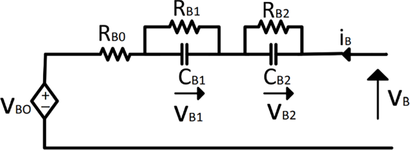
Figure 23: Diagram of a circuit battery
The greater the number of parallel RC circuits in series, the higher the accuracy of the model, although it is found that the series connection of two parallel RC circuits provides fairly reliable dynamic performance with reduced computational complexity. There are only two batteries with RC modules connected in parallel. The following are differential equations and algebraic equations describing battery dynamics.
4.7 Electric Vehicle Dynamic Load Model
The model of the dynamic load EV can be established by taking into account the analysis in Sections 4.2–4.6. The dynamic load EV model can be defined using the eleventh-order model presented in the differential Eqs. (109) and algebra (110).
4.8 Small Signal Stability Analysis with Dynamic EV Load Representation
This section contains the model established in Section 4.4 to estimate the effect of EV charging on weak signal stability in the power system. The analysis considers the modified SMIB with a load bus test system, see Fig. 24, and the classic model with a synchronous Machine Model.
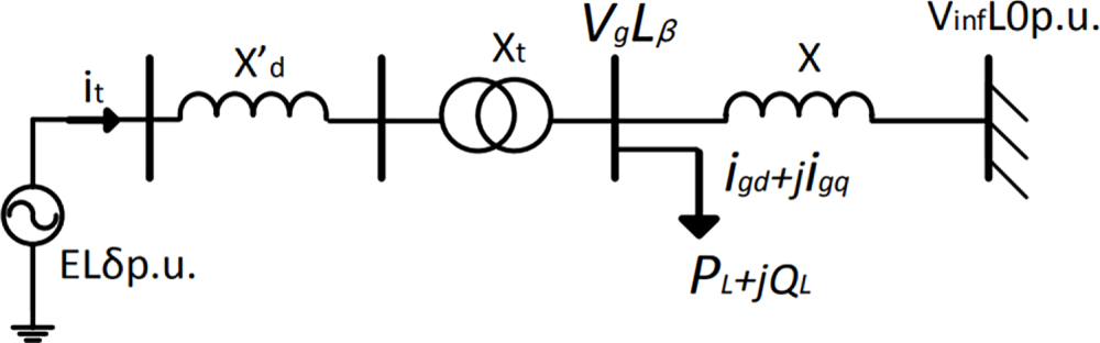
Figure 24: Modified SMIB model
The electrical power output of the synchronous generator (Pe) is determined as,
Or,
The linearized power output can be written as in (62)
The bus voltage vg can be defined in the dq frame by (115), and linearized vg is described as in (116).
Now vgd and vgq can be linearized as in (118) and (119),
Considering only the imaginary part of (117),
On linearizing the (121) results (122)
On linearizing id and iq we get Eqs. (126) and (127)
Now referencing in global quantities, we get
Linearized equations of (123) and (124)
Linearized differential Eqs. (136) and (146) can be expressed by the matrix shown in (147). By analyzing the eigenvalues of the system state matrix, the impact of the EV charging load on the stability of the weak signal of the system is estimated (Asys) as shown in (147).
4.9 Analysis of Small Signal Stability of SMIB Connected with EV and UPFC
The small signal stability of the SMIB system is evaluated in this section when it is connected to EV and UPFC. The system model is defined by a tenth-order model characterized by the state space model Eq. (148).
where
The performance of the SMIB with the UPFC system is carried out by using software called MATLAB/SIMULINK.
Generator:
Excitation system:
Transformer:
Transmission line:
Operating conditions:
UPFC parameters:
From Fig. 24a,b, it is confirmed that the LQR control with proper tuning of Q and R matrices gives a really good response.
EV Load Model Parameters
The eigenvalues and damping ratios of the electromechanical mode are available in Tables 7 and 8 when it is exposed to different operating constraints.
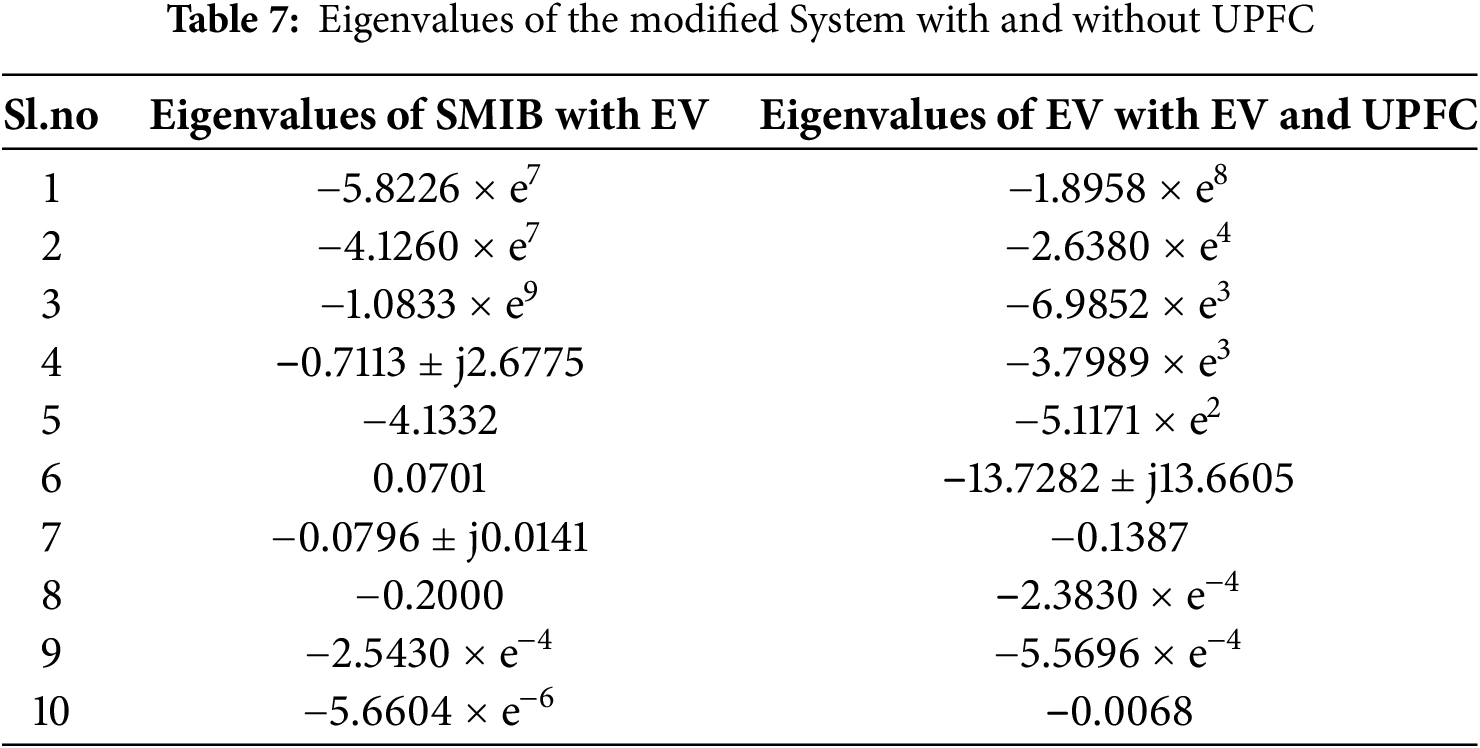
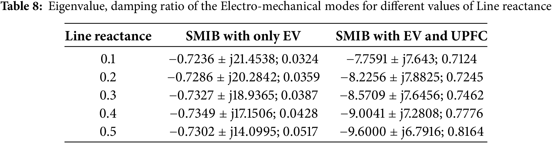
Fig. 25 demonstrates that as the value of Xe is increased, the corresponding eigenvalue tends to move away from the origin, i.e., the eigenvalues tend to move towards the left-hand side (LHS) of the s-plane, which implies the damping ratios and system stability are improved.
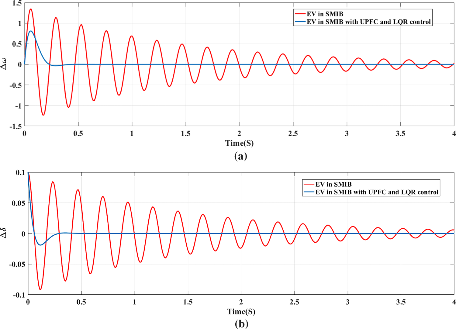
Figure 25: (a) Rotor speed deviation in the SMIB system with EV and EV with LQR Control. (b) Deviation in rotor speed in the SMIB system with EV and EV with LQR Control
Fig. 25 and Table 7 demonstrate that as the value of X ~e~ is increased, which implies the damping ratios and system stability are improved. This analysis also provides insight into how system strength (inversely related to reactance) affects stability when integrated with EV loads.
6 Conclusion and Future Scope of the Work
This work considered optimal control-based small signal stability analysis of power systems, including the Flexible AC Transmission System and electric vehicle charging load. Charging electric vehicles brings many challenges to the power system, and it has been found that the voltage-dependent charging behaviour of electric vehicles not only affects the stability of the system voltage but also affects the small signal stability of the power system. It is helpful to take action when planning an electric car charger. The results show that charging an EV will have a negative effect on the small signal stability of the system. Therefore, when planning an electric vehicle charger, it is important to consider the small signal stability part of the system. Since these state variables are connected to the battery and DC/DC converter control system, a suitably tuned DC/DC converter controller seems to minimize the impact. The results demonstrated that the system response using a modified Single Machine Infinite Bus power system with a Unified Power Flow Controller and Linear Quadratic Regulator control gives better response with decreased settling time, rise time, and peak overshoot.
The results demonstrated that the system response using a modified Single Machine Infinite Bus power system with a Unified Power Flow Controller and Linear Quadratic Regulator control gives a superior response compared to the system with only a PSS, with quantitatively decreased settling time, rise time, and peak overshoot.
While the proposed LQR-UPFC scheme demonstrates excellent performance in simulation, several practical implementation challenges must be considered for real-world deployment. These include the computational burden of solving the Riccati equation for large-scale systems, communication delays in wide-area control signals, and sensitivity to system parameter uncertainties, which could affect controller robustness. Furthermore, this study assumes full state feedback, which may not always be available, necessitating the use of state observers in practice.
The scope of future work is determined by:
• Power System Stabilizer is a very costly device, and it will not be economical to install Power System Stabilizer in every synchronous generator. The number of Power System Stabilizers can be optimized for more economical operation, considering the stability of the system.
• Also, the other Flexible AC Transmission System controllers like Static VAR Compensator, Thyristor Controlled Series Capacitor, etc., can be designed to improve stability, and they can be coordinated with the Power System Stabilizer also.
• Optimal coordinated design of multiple damping controllers based on Power System Stabilizers and Unified Power Flow Controller device can achieve dynamic stability.
• The renewable energy sources, e.g., solar photovoltaic and wind, could be considered in a large multi-area system. Hence, the stochastic study of the system can be performed to obtain more accurate results than the deterministic approach.
Acknowledgement: Not applicable.
Funding Statement: The authors received no specific funding for this study.
Author Contributions: The authors confirm contribution to the paper as follows: Naveen Guguloth: Conceptualization; Methodology; Formal analysis; Investigation; Data curation; Software, Supervision, Validation; Writing—original draft; Writing—reviewing & editing. Prasenjit Dey: Methodology; Formal analysis; Investigation; Data curation; Software, Supervision, Validation; Writing—original draft; Bishwajit Dey: Conceptualization; Formal analysis; Investigation; Data curation; Software, Supervision, Validation; Writing—reviewing & editing. Isaac Segovia Ramírez: Funding acquisition; Methodology, Project administration; Resources; Software; Supervision; Writing—reviewing & editing. Fausto Pedro García Márquez: Conceptualization; Funding acquisition; Methodology, Project administration; Resources; Software; Supervision; Validation; Writing—original draft; Writing—reviewing & editing. All authors reviewed and approved the final version of the manuscript.
Availability of Data and Materials: The data that support the findings of this study are available from the Corresponding Author, upon reasonable request.
Ethics Approval: Not applicable.
Conflicts of Interest: The authors declare no conflicts of interest to report regarding the present study.
Abbreviations
| ARE | Algebraic Riccati Equation |
| AVR | Automatic Voltage Regulator |
| BEV | Battery Electric Vehicle |
| BT | Boosting Transformer |
| CAFE | Corporate Average Fuel Economy |
| CC-CV | Constant Current and Constant Voltage |
| EV | Electric Vehicle |
| FACTS | Flexible AC Transmission System |
| HEV | Hybrid Electric Vehicle |
| IPFC | Interline Power Flow Controller |
| ML | Machine Learning |
| LFO | Low-Frequency Oscillations |
| LQR | Linear Quadratic Regulator |
| PHEV | Plug-in Hybrid Electric Vehicle |
| POD | Power Oscillation Damper |
| PSS | Power System Stabilizer |
| PV | Photovoltaic |
| PWM | Pulse Width Modulation |
| SMIB | Single Machine Infinite Bus |
| SOC | State of Charge |
| SSSC | Static Synchronous Series Compensator |
| SVC | Static VAR Compensator |
| TCSC | Thyristor Controlled Series Capacitor |
| UPFC | Unified Power Flow Controller |
References
1. Asif M, Muneer T. Energy supply, its demand and security issues for developed and emerging economies. Renew Sustain Energy Rev. 2007;11(7):1388–413. doi:10.1016/j.rser.2005.12.004. [Google Scholar] [CrossRef]
2. García Márquez FP, Segovia Ramírez I, Pliego Marugán A. Decision making using logical decision tree and binary decision diagrams: a real case study of wind turbine manufacturing. Energies. 2019;12(9):1753. doi:10.3390/en12091753. [Google Scholar] [CrossRef]
3. Sánchez PJB, Asensio MT, Papaelias M, Márquez FPG. Life cycle assessment in autonomous marine vehicles. In: Proceedings of the Fifteenth International Conference on Management Science and Engineering Management. Cham, Switzerland: Springer International Publishing; 2021. p. 222–33. doi:10.1007/978-3-030-79206-0_17. [Google Scholar] [CrossRef]
4. Jenkins N. Embedded generation. Power Eng J. 1995;9(3):145–50. doi:10.1049/pe:19950309. [Google Scholar] [CrossRef]
5. García Márquez FP, Segovia Ramírez I, Mohammadi-Ivatloo B, Marugán AP. Reliability dynamic analysis by fault trees and binary decision diagrams. Information. 2020;11(6):324. doi:10.3390/info11060324. [Google Scholar] [CrossRef]
6. García Márquez FP, Schmid F, Collado JC. Wear assessment employing remote condition monitoring: a case study. Wear. 2003;255(7–12):1209–20. doi:10.1016/s0043-1648(03)00214-x. [Google Scholar] [CrossRef]
7. Taylor P. Energy technology perspectives. Int Energy Agency. 2010;692:1–19. [Google Scholar]
8. Allcock C, Barghout J, Drye K. EV City Case Book [Internet]. [cited 2025 Nov 1]. Available from: https://www.osti.gov/etdeweb/biblio/22112376. [Google Scholar]
9. Khaleel M, Nassar Y, El-Khozondar HJ, Elmnifi M, Rajab Z, Yaghoubi E, et al. Electric vehicles in China, Europe, and the United States: current trend and market comparison. Int J Electr Eng Sustain. 2024;2:1–20. [Google Scholar]
10. Global EV Outlook 2024. Paris, France: International Energy Agency; 2024. [Google Scholar]
11. Kundur P. Power systems stability and control. New York, NY, USA: McGraw-Hi1l; 2022. [Google Scholar]
12. Sauer P, Pai M. Power system dynamics and stability. Upper Saddle River, NJ, USA: Prentice Hall; 1997. [Google Scholar]
13. Dey B, Raj S, Mahapatra S, Márquez FPG. Optimal scheduling of distributed energy resources in microgrid systems based on electricity market pricing strategies by a novel hybrid optimization technique. Int J Electr Power Energy Syst. 2022;134:107419. doi:10.1016/j.ijepes.2021.107419. [Google Scholar] [CrossRef]
14. Padiyar K. Power system dynamics. Hyderabad, India: BS Publications; 2008. [Google Scholar]
15. Anderson PM, Fouad AA. Power system control and stability. Hoboken, NJ, USA: John Wiley & Sons, Inc.; 2008. [Google Scholar]
16. Pai M, Gupta DS, Padiyar K. Small signal analysis of power systems. Oxford, UK: Alpha Science Int’l Ltd.; 2004. [Google Scholar]
17. Hingorani NG, Gyugyi L. Understanding FACTS: concepts and technology of flexible AC transmission systems. Piscataway, NJ, USA: Wiley-IEEE Press; 2000. [Google Scholar]
18. Zarghami M, Crow ML, Jagannathan S. Nonlinear control of FACTS controllers for damping interarea oscillations in power systems. IEEE Trans Power Deliv. 2010;25(4):3113–21. doi:10.1109/TPWRD.2010.2055898. [Google Scholar] [CrossRef]
19. Tang Y, Meliopoulos APS. Power system small signal stability analysis with FACTS elements. IEEE Trans Power Deliv. 1997;12(3):1352–61. doi:10.1109/61.637014. [Google Scholar] [CrossRef]
20. Bindal RK. A review of benefits of FACTS devices in power system. Int J Eng Adv Technol. 2014;3(4):105–8. [Google Scholar]
21. Yu Z, Yang C, Wang Q. The impact of large-scale EV charging on the real-time operation of distribution systems: a comprehensive review. arXiv:2507.21759. 2025. [Google Scholar]
22. Sun L, Teh J, Liu W, Lai CM, Chen LR. Impact of electric vehicles on power system reliability and related improvements: a review. Electr Power Syst Res. 2025;247:111838. doi:10.1016/j.epsr.2025.111838. [Google Scholar] [CrossRef]
23. Su Y, Teh J. Two-stage optimal dispatching of AC/DC hybrid active distribution systems considering network flexibility. J Mod Power Syst Clean Energy. 2023;11(1):52–65. doi:10.35833/mpce.2022.000424. [Google Scholar] [CrossRef]
24. Prakash A, El Moursi MS, Parida SK, Kumar K, El-Saadany EF. Damping of inter-area oscillations with frequency regulation in power systems considering high penetration of renewable energy sources. IEEE Trans Ind Appl. 2024;60(1):1665–79. doi:10.1109/TIA.2023.3312061. [Google Scholar] [CrossRef]
25. Tayri A, Ma X. Grid impacts of electric vehicle charging: a review of challenges and mitigation strategies. Energies. 2025;18(14):3807. doi:10.3390/en18143807. [Google Scholar] [CrossRef]
26. Gautam M. Deep reinforcement learning for resilient power and energy systems: progress, prospects, and future avenues. Electricity. 2023;4(4):336–80. doi:10.3390/electricity4040020. [Google Scholar] [CrossRef]
27. Mohamed TH, Bevrani H, Hassan AA, Hiyama T. Decentralized model predictive based load frequency control in an interconnected power system. Energy Convers Manag. 2011;52(2):1208–14. doi:10.1016/j.enconman.2010.09.016. [Google Scholar] [CrossRef]
28. Liu J, Yao Q, Hu Y. Model predictive control for load frequency of hybrid power system with wind power and thermal power. Energy. 2019;172:555–65. doi:10.1016/j.energy.2019.01.071. [Google Scholar] [CrossRef]
29. Khamies M, Magdy G, Kamel S, Khan B. Optimal model predictive and linear quadratic Gaussian control for frequency stability of power systems considering wind energy. IEEE Access. 2021;9:116453–74. doi:10.1109/access.2021.3106448. [Google Scholar] [CrossRef]
30. Komurcugil H, Biricik S, Bayhan S, Zhang Z. Sliding mode control: overview of its applications in power converters. IEEE Ind Electron Mag. 2021;15(1):40–9. doi:10.1109/MIE.2020.2986165. [Google Scholar] [CrossRef]
31. Wu L, Liu J, Vazquez S, Mazumder SK. Sliding mode control in power converters and drives: a review. IEEE/CAA J Autom Sin. 2022;9(3):392–406. doi:10.1109/jas.2021.1004380. [Google Scholar] [CrossRef]
32. Yin Y, Liu J, Sánchez JA, Wu L, Vazquez S, Leon JI, et al. Observer-based adaptive sliding mode control of NPC converters: an RBF neural network approach. IEEE Trans Power Electron. 2019;34(4):3831–41. doi:10.1109/TPEL.2018.2853093. [Google Scholar] [CrossRef]
33. Sebaaly F, Vahedi H, Kanaan HY, Moubayed N, Al-Haddad K. Design and implementation of space vector modulation-based sliding mode control for grid-connected 3L-NPC inverter. IEEE Trans Ind Electron. 2016;63(12):7854–63. doi:10.1109/TIE.2016.2563381. [Google Scholar] [CrossRef]
34. Shamsollahi P, Malik OP. Design of a neural adaptive power system stabilizer using dynamic back-propagation method. Int J Electr Power Energy Syst. 2000;22(1):29–34. doi:10.1016/s0142-0615(99)00032-0. [Google Scholar] [CrossRef]
35. Sharma G, Panwar A, Arya Y, Kumawat M. Integrating layered recurrent ANN with robust control strategy for diverse operating conditions of AGC of the power system. IET Gener Transm Distrib. 2020;14(18):3886–95. doi:10.1049/iet-gtd.2019.0935. [Google Scholar] [CrossRef]
36. Bigdeli N, Ghanbaryan E, Afshar K. Low frequency oscillations suppression via CPSO based damping controller. J Operat Automat Power Engi. 2013;1(1):22–32. [Google Scholar]
37. Chakrabarti A, Halder S. Power system analysis: operation and control. 3rd ed. Delhi, India: PHI Learning Pvt. Ltd.; 2010. [Google Scholar]
38. Ho Y-C. Applied optimal control: optimization, estimation, and control. Hoboken, NJ, USA: Halsted Press; 1975. [Google Scholar]
39. Marquez FPG. An approach to remote condition monitoring systems management. In: Proceedings of the 2006 IET International Conference on Railway Condition Monitoring; 2006 Nov 29–30; Birmingham, UK. p. 156–60. doi:10.1049/ic:20060061. [Google Scholar] [CrossRef]
40. Oral Ö, Çetin L, Uyar E. A novel method on selection of Q and R matrices in the theory of optimal control. Int J Syst Cont. 2010;1(2):84. [Google Scholar]
41. Kumkratug P. Power system stability controls. In: Power system stability and control. Boca Raton, FL, USA: CRC Press; 2007. p. 169–88. doi:10.1201/9781420009248-18. [Google Scholar] [CrossRef]
42. Rezazadeh A, Sedighizadeh M, Hasaninia A. Coordination of PSS and TCSC controller using modified particle swarm optimization algorithm to improve power system dynamic performance. J Zhejiang Univ Sci C. 2010;11(8):645–53. doi:10.1631/jzus.c0910551. [Google Scholar] [CrossRef]
43. Pal B, Chaudhuri B. Robust control in power systems. New York, NY, USA: Springer Science & Business Media; 2006. [Google Scholar]
44. Kumkratug P. Power system stability enhancement using unified power flow controller. Am J Appl Sci. 2017;7:1504–8. doi:10.3844/AJASSP.2010.1504.1508. [Google Scholar] [CrossRef]
45. Chow JH, Sanchez-Gasca JJ, Ren H, Wang S. Power system damping controller design-using multiple input signals. IEEE Control Syst Mag. 2000;20(4):82–90. doi:10.1109/37.856181. [Google Scholar] [CrossRef]
46. Taher SA, Abrishami AA. UPFC location and performance analysis in deregulated power systems. Math Probl Eng. 2009;2009(1):109501. doi:10.1155/2009/109501. [Google Scholar] [CrossRef]
47. Wang H, Xu H. FACTS-based stabilizers to damp power system oscillations—a survey. In: Proceedings of the 39th International Universities Power Engineering Conference, 2004; 2004 Sep 6–8; Bristol, UK. p. 318–22. [Google Scholar]
48. Dharmakeerthi CH, Mithulananthan N, Saha TK. Overview of the impacts of plug-in electric vehicles on the power grid. In: 2011 IEEE PES Innovative Smart Grid Technologies; 2011 Nov 13–16; Perth, WA, Australia. p. 1–18. doi:10.1109/ISGT-Asia.2011.6167115. [Google Scholar] [CrossRef]
49. SAE Hybrid Committee. SAE charging configurations and ratings terminology. Troy, MI, USA: Society of Automotive Engineers; 2011. [Google Scholar]
50. Bauer P, Stembridge N, Doppler J, Kumar P. Battery modeling and fast charging of EV. In: Proceedings of 14th International Power Electronics and Motion Control Conference EPE-PEMC 2010; 2010 Sep 6–8; Ohrid, Macedonia. p. S11-39–45. doi:10.1109/EPEPEMC.2010.5606530. [Google Scholar] [CrossRef]
51. Wong WC, Chung CY, Chan KW, Chen H. Quasi-Monte Carlo based probabilistic small signal stability analysis for power systems with plug-in electric vehicle and wind power integration. IEEE Trans Power Syst. 2013;28(3):3335–43. doi:10.1109/TPWRS.2013.2254505. [Google Scholar] [CrossRef]
52. Kuperman A, Levy U, Goren J, Zafranski A, Savernin A, Peled I. Modeling and control of a 50KW electric vehicle fast charger. In: 2010 IEEE 26-th Convention of Electrical and Electronics Engineers in Israel; 2010 Nov 17–20; Eilat, Israel. p. 188–92. doi:10.1109/EEEI.2010.5661955. [Google Scholar] [CrossRef]
53. Young K, Wang C, Wang LY, Strunz K. Electric vehicle battery technologies. In: Electric vehicle integration into modern power networks. New York, NY, USA: Springe; 2012. p. 15–56. doi:10.1007/978-1-4614-0134-6_2. [Google Scholar] [CrossRef]
Cite This Article
 Copyright © 2026 The Author(s). Published by Tech Science Press.
This work is licensed under a Creative Commons Attribution 4.0 International License , which permits unrestricted use, distribution, and reproduction in any medium, provided the original work is properly cited.
 Downloads
 Citation Tools