EB-Guided Optimization of Heliostat Fields with Validated Projection Losses and HFLCAL Sensitivity

1  Introduction

Central receiver (power tower) plants concentrate direct normal irradiance (DNI) via large heliostat fields onto an elevated receiver. Decisions at the field level—ring radii, azimuthal spacing, mirror aperture, and installation height—propagate through the optical chain (cosine, shading/blocking, atmospheric attenuation, truncation/receiver intercept) into delivered thermal power and annual energy yield [1]. As deployment scales up, developers require workflows that (i) keep geometric and optical conventions consistent, (ii) combine fast but calibrated optical surrogates with selective ray tracing, and (iii) search high-dimensional layouts efficiently under engineering constraints.

1.1 Layout Archetypes and Field Geometry

Early surround or north-field patterns often used radial or staggered lattices with hand-tuned spacing rules. Biomimetic and density-graded schemes (e.g., equalizing beam density at the receiver plane rather than ground density) sought better cosine efficiency and reduced inter-ring occlusions [2]. Reviews emphasize that field geometry trades off multiple effects: moving heliostats outward improves cosine efficiency near noon but increases attenuation and truncation; tighter azimuthal packing raises shading/blocking (SB) at low solar altitudes; ring heights can relieve near-neighbor blocking at the cost of structure and tracking errors [1]. Contemporary practice combines a parametric ring skeleton (radii/azimuthal spacing laws) with local spacing rules that enforce collision-free kinematics and service corridors.

1.2 Optical Modeling: Analytical Chains vs. Ray Tracing

Analytical chains remain attractive for speed and differentiability. A representative factorization is

ηi=ηcos,iηsb,iηat,iηtrunc,iηref,(1)

with cosine loss from incident/normal geometry, SB losses from projected overlaps, atmospheric transmittance parameterized by path length, and receiver intercept modeled via HFLCAL (an analytic heliostat-field local calculation model for flux and truncation) sunshape/blur footprints [3–5]. HFLCAL encapsulates sunshape, slope/astigmatism, and tracking errors into a Gaussian (or near-Gaussian) convolution whose variance scales with range, yielding closed-form or quickly evaluated receiver intercept terms that are convenient in layout optimization [3,4]. High-fidelity Monte-Carlo ray tracers (SolTrace, Tonatiuh/Tonatiuh2) provide reference benchmarks for optical accuracy and are routinely used to validate simplified chains at selected sun positions and for representative neighbor constellations [6–8]. This calibration loop—fast chain for the search, ray tracing for spot checks—is now common in industrial toolchains [9].

1.3 Shading/Blocking Computation

SB losses dominate when azimuthal packing is high or when the sun is low. Exact polygon-overlap on the mirror plane after 3D projection is widely used in research prototypes and embedded tools, striking a balance between speed and modeling fidelity for rectangular heliostats [10]. Efficient implementations prune neighbor sets by range/angle cones and test only candidates likely to overlap in projection, which preserves O(N) behavior at fixed field density. The literature further distinguishes shading (incident direction) from blocking (reflected direction toward the receiver), suggesting that nearest-ring neighbors contribute the bulk of the loss under typical aiming strategies. This motivates ring-aware pruning in large fields [2,11].

1.4 Atmospheric Transmittance and Truncation/Intercept

Short-range towers often use empirical transmittance curves that depend on the heliostat-receiver path length. At kilometer-scale ranges, exponential or quadratic fits are adequate surrogates for clear-sky conditions in annual energy estimates. For the receiver intercept, HFLCAL-style formulations propagate a composite blur—sunshape, slope error, astigmatism, and tracking error—to the receiver plane and then integrate over the aperture to obtain ηtrunc [3–5]. Reviews and progress reports note that improvements in optical surfaces and control systems reduce the contributions from tracking error and slope error, which increases the relative importance of sunshape and aiming dispersion for the peak-to-mean flux and for thermal feasibility [1].

1.5 Optimization Algorithms and Software Support

Because field layout is high-dimensional and nonconvex, metaheuristics are common. Classical GA/NSGA-II, PSO, and GWO remain strong baselines for multiobjective trade-offs between annual energy, peak flux, land use, and cost proxies [12,13]. Newer swarms (e.g., coyote optimization) and problem-specific hybrids seek faster convergence by mixing global exploration with local refinements [14]. Industrial tools such as SolarPILOT operationalize ring generation, spacing, SB, aiming, and flux maps, enabling practitioners to combine optimizers with validated optics and controls in one loop [9]. Two-step frameworks decouple ring-level geometry from local spacing/final aiming to cut search complexity and improve robustness [11]. Complementary control-side advances in multi-point aiming improve flux uniformity and reduce thermal constraint violations during transients [15].

1.6 Reliability, Roadmaps, and Modeling Implications

Recent gap analyses and roadmaps consolidate field evidence on component reliability, cost, and error budgets across drives, structures, and mirrors [16,17]. For modeling, these reports motivate four aspects: (i) explicit accounting of tracking and slope error distributions within the HFLCAL variance budget, (ii) height- and structure-related constraints that prevent unrealistic occlusion fixes, (iii) practical spacing corridors for operations and maintenance, and (iv) flux caps or soft penalties at the panel level that reflect thermal durability constraints. They also highlight the value of auditable pipelines that combine fast analytical models with targeted ray-tracing validation.

1.7 Gaps Addressed in This Work

Despite steady progress, three gaps persist in the literature and practice:

1.   Consistent geometry and optics. Many studies mix coordinate conventions, sun/azimuth definitions, or partial optical chains, hampering reproducibility and cross-study comparisons. We adopt a single East–North–Up (ENU) convention and a factorized chain calibrated by ray tracing [6,8].

2.   SB and intercept coupling in the search. Layouts are often tuned on cosine/attenuation while treating SB and truncation post-hoc. We integrate projection-based SB and HFLCAL intercept directly into the objective and constraints [3,4].

3.   Search efficiency under constraints. General-purpose swarms can be slow when enforcing spacing, kinematics, and flux limits. We guide the search with an Eliminate-Blocking (EB) prior for ring/azimuth scaling and combine fast exploration with elite-focused refinements, retaining parity with GA/PSO/GWO evaluation budgets [11–14].

Our contributions.

•   A unified, auditable pipeline that (i) fixes ENU geometry and solar conventions, (ii) fuses cosine, SB (projection), atmospheric transmittance, and HFLCAL truncation, and (iii) cross-checks against open ray tracers at representative suns [6,8].

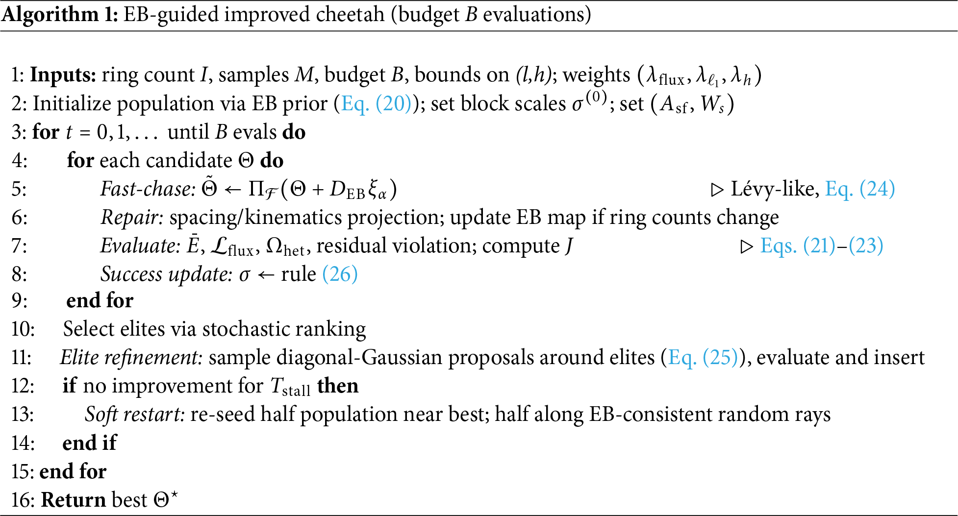
•   An EB-guided improved “Cheetah” metaheuristic that encodes outward-increasing azimuthal spacing and alternates fast exploration with elite refinements, while enforcing spacing/kinematics and panel-level flux penalties consistent with industrial practice [9,15].

•   A three-phase study (fixed-size baseline, uniform sizing, heterogeneous sizing) showing stable convergence and higher annual per-area output vs. a radial baseline, consistent with system-level insights reported in recent reviews and roadmaps [1,17].

Figures used in this section. Fig. 1 establishes the ENU frame used throughout; Fig. 2 sketches the solar angles and hour-angle convention.

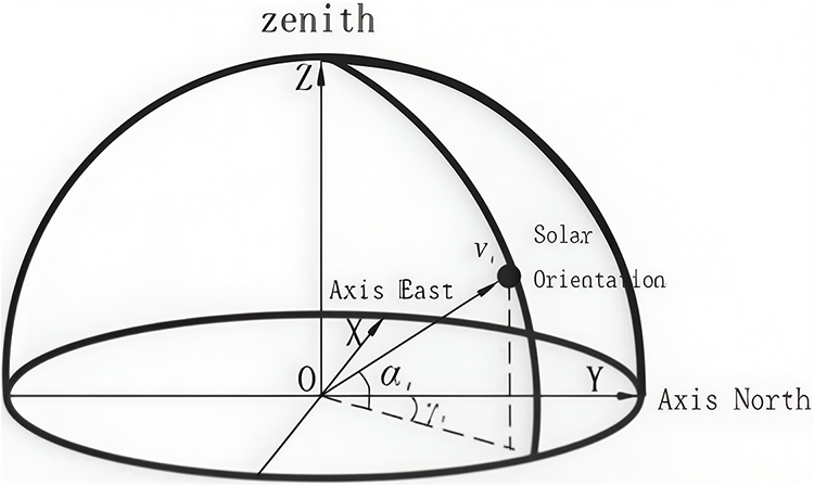
Figure 1: Field coordinate system (East–North–Up) and solar-orientation definitions

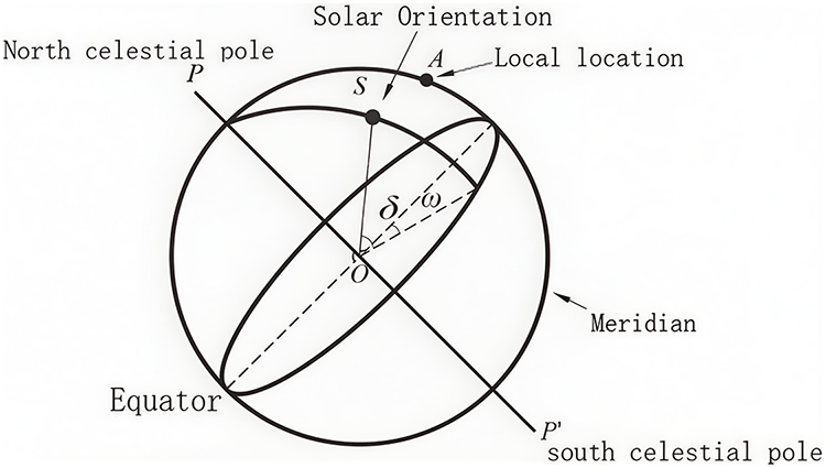
Figure 2: Celestial-sphere sketch showing declination δ and hour angle ω

2  Related Work and Motivation

Designing heliostat fields sits at the intersection of geometry, optics, controls, and optimization. Prior research offers a variety of field archetypes, surrogate optical models, and optimizers, while industrial toolchains operationalize many of these ideas. This section reviews what is known and motivates the specific modeling and optimization choices adopted in this work.

2.1 Layout Archetypes and Trade-Offs

Early surround fields often used radial or north-field lattices with ring-wise staggering to mitigate low-sun occlusions, and then layered local spacing rules to preserve operations and maintenance corridors and collision-free kinematics. Biomimetic and density-graded layouts improved cosine efficiency and reduced near-neighbor shading and blocking (SB) by shaping azimuthal spacing as a function of range [1,2]. Eliminate-Blocking (EB) layouts go a step further. In these schemes, as implemented for example in SolarPILOT and related field-design tools [9,11], the ring radii and azimuthal separations are chosen such that the blocking factor remains approximately constant across rings for a set of design sun positions. In practice, this outward-growing azimuthal spacing also tends to mitigate near-neighbor shading and blocking (SB) and to produce a more uniform beam density at the receiver plane under first-order optics. These effects are visible later in the optimized layouts shown in Section 6. Reviews stress that no single geometry dominates across sites. Rather, cosine, SB, attenuation, and truncation interact in a way that depends on both the site and the receiver configuration [1]. Throughout this paper, EB therefore denotes an Eliminate-Blocking layout rule rather than an equal-ground-density pattern.

2.2 Analytical Optical Chains vs. Ray Tracing

Analytical chains factorize optical efficiency as

ηi=ηcos,iηsb,iηat,iηtrunc,iηref,(2)

providing speed and differentiability required by optimizers. Common choices include geometry-based cosine, polygon-overlap SB on the mirror plane, empirical clear-sky attenuation with path length, and HFLCAL-style intercept (receiver truncation) [3–5]. Because these surrogates simplify wavefront and scatter physics, selective high-fidelity validation is routine: Monte-Carlo ray tracers (SolTrace, Tonatiuh/Tonatiuh2) serve as reference models to calibrate surrogate parameters and to check worst-case constellations [6–8]. Industrial software (SolarPILOT) packages this workflow by combining ring generation, aiming, flux maps, and optimizer hooks [9].

2.3 Shading/Blocking Computation

The projection-based SB computation is illustrated in Figs. 3 and 4, which show the 3D projection and its 2D top-view overlap geometry, respectively. SB losses dominate when the sun is low or azimuthal packing is tight. Projection-based SB treats each neighbor pair by projecting polygonal apertures along the incident direction to compute shading, and along the reflected direction toward the receiver to compute blocking. Two-dimensional polygon overlaps on the target mirror yield fractional loss areas. Efficient implementations prune candidates using angular cones and distance thresholds because nearest-ring neighbors account for most SB [2,11]. Although ray tracing can capture mirror thickness, canting errors, and edge diffraction, projection-based SB achieves excellent runtime and sufficient fidelity for optimization loops when it is periodically cross-checked against ray-tracing overlaps [6] (Figs. 3 and 4).

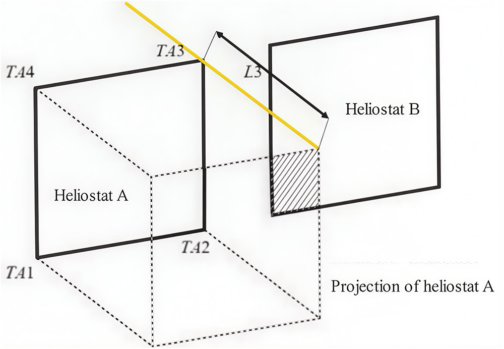
Figure 3: Projection-based shading/blocking between heliostats (hatched overlap on B)

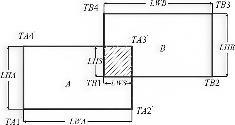
Figure 4: Top-view 2D overlap geometry corresponding to the projection model

2.4 Receiver Intercept (HFLCAL Truncation) and Flux Quality

HFLCAL-style models represent the image on the receiver as a convolution of sunshape with blur terms due to slope and astigmatism and tracking, and the composite variance grows with the heliostat–receiver range. Integrating the resulting footprint over the aperture gives ηtrunc that is fast to evaluate and differentiable, which makes it attractive inside optimizers [3,4]. Reviews and progress reports note that as mechanical and control quality improves, sunshape and aiming dispersion increasingly govern peak-to-mean flux and thermal margins [1]. In practice, the intercept should be coupled to layout and aiming decisions. Decoupling can bias ring density outward (lower SB) at the cost of increased spread and truncation. Our pipeline keeps HFLCAL inside the objective to expose this trade-off to the search.

2.5 Atmospheric Transmittance and Path-Length Effects

For tower ranges below a few kilometers, empirical fits of transmittance vs. path length (linear/quadratic/exponential) provide adequate clear-sky proxies and are widely used in annual-energy estimators and screening studies [5]. Because attenuation grows with range, outer-ring gains from better cosine and reduced SB must be balanced against transmittance and truncation penalties.

2.6 Optimization Frameworks and Software Practice

Heliostat layout is high dimensional and nonconvex, with discrete variables (counts per ring) and continuous variables (radii, azimuths, sizes, heights), together with hard constraints on spacing and kinematics. Metaheuristics are therefore prevalent. Genetic algorithms (including NSGA-II), particle swarm optimization, and the grey wolf optimizer remain strong baselines for single-objective and multi-objective settings [12,13]. Newer swarms, such as the coyote optimization algorithm, improve exploration by sharing information within subgroups [14]. Toolchains such as SolarPILOT integrate these optimizers with shading and blocking and with aiming modules, which enables rapid prototyping and comparative studies [9]. Two-step frameworks reduce search complexity by first laying out ring skeletons and then refining local spacing and aiming under the optical model [11]. Complementary control strategies, including multi-point aiming and flux shaping, further reduce peak flux while preserving intercept [15,18,19].

2.7 Engineering Constraints, Reliability, and Modeling Implications

Recent roadmaps and gap analyses synthesize field experience across drives, structure, mirrors, and control, offering quantitative error budgets (tracking, slope) and reliability priorities that should inform models and constraints [16,17]. From a modeling standpoint, this motivates: (i) explicit inclusion of tracking/slope statistics in the HFLCAL variance budget; (ii) height and spacing rules that are realistic for structure and O&M; (iii) flux caps or soft penalties to reflect receiver durability; and (iv) auditable pipelines that mix fast surrogates with targeted ray-trace checks.

2.8 Motivation and Problem Statement

Despite decades of advances, three practical gaps remain:

1.   Consistency across geometry and optics. Studies sometimes mix coordinate conventions and partial optical chains, complicating replication. We adopt a single ENU convention (Figs. 1 and 2) and a factorized chain (cosine, SB via projection, attenuation, HFLCAL intercept) validated against open ray tracers [6,8].

2.   Coupling SB and intercept in the search. Optimizers frequently tune cosine/attenuation while treating SB/intercept as post-processing, which can bias solutions. We embed projection-based SB and HFLCAL within the objective and constraints, exposing their trade-offs during search [3,4].

3.   Search efficiency under engineering constraints. Generic swarms slow down when enforcing spacing/kinematics and flux penalties. We guide the search with an EB prior (outward-growing azimuthal spacing) and use an improved “Cheetah”-style metaheuristic to alternate fast exploration with elite refinement under equal evaluation budgets, keeping parity with GA/PSO/GWO [11–14].

Scope in this work.

We build an auditable pipeline that (i) fixes geometry and optical conventions, (ii) integrates SB, attenuation, and HFLCAL into the objective, (iii) validates surrogate SB against ray tracing at representative sun positions, and (iv) uses an EB-guided optimizer to search ring topology, sizes, and heights with realistic spacing and kinematics. The subsequent sections detail the models with equations, the experimental protocol, and the phase-wise results, while Figs. 3 and 4 visualize the SB geometry, and the resulting EB layouts are shown later in Section 6.

3  Methods

3.1 Solar Geometry and Frames

We adopt a ground-fixed East-North-Up (ENU) coordinate system: x points East, y points North, and z points upward. The receiver center is O=(0,0,Hz). A heliostat center is A=(xA,yA,zA). With day-of-year D,

δ(D)=23.45∘sin(2π365(284+D)).(3)

Given solar time ST (hours), the hour angle is ω=15∘(ST−12). With latitude φ,

αs=arcsin⁡(cos⁡δcos⁡φcos⁡ω+sin⁡δsin⁡φ),(4)

γs=arccos(sin⁡δ−sin⁡αssin⁡φcos⁡αscos⁡φ).(5)

At A define Si(αs,γs), Sr=(O−A)/‖O−A‖, and Sn=(Sr−Si)/‖Sr−Si‖. The cosine efficiency is ηcos=|Si⋅Sn|.

All top-view layouts and overlap diagrams in this paper follow this ENU convention unless stated otherwise.

3.2 Optical Chain

For heliostat i,

ηi=ηcos,iηsb,iηat,iηtrunc,iηref,ηref=0.92.(6)

Projection-based shading/blocking (SB).

For each pair (A,B), we project heliostat A along the incident direction onto the plane of B to compute shading, and we project B along the reflected direction toward the receiver to compute blocking. As sketched in Fig. 3, TA1–TA4 denote the four vertices of heliostat A in 3D, and the dashed lines show their projection onto the plane of heliostat B. The segment labeled L3 lies along the incident ray and represents the distance between the intersection with the front heliostat A and the plane of the back heliostat B, which determines the relative displacement of the projected polygon on B. In B’s local 2D frame, the projected rectangles of A and B overlap to form a shading or blocking polygon. Summing over neighbors yields

ηsb,B=1−∑i∈𝒩(B)Δηi→Bshade−∑i∈𝒩(B)Δηi→Bblock.(7)

For rectangles with projected spans [xA1,xA2], [xB1,xB2] and [yA1,yA2], [yB1,yB2]:

LW=(xA2−xA1)+(xB2−xB1)−(max(xA2,xB2)−min(xA1,xB1)),(8)

LH=(yA2−yA1)+(yB2−yB1)−(max(yA2,yB2)−min(yA1,yB1)),(9)

and Δη=(LWLH)/AB if LW,LH>0, else 0. Fig. 4 shows the corresponding top-view rectangles A and B: TA1′–TA4′ and TB1–TB4 are their vertices in the local 2D frame, LHA and LWA are the projected height and width of heliostat A, LHB and LWB are those of heliostat B, and LHS and LWS denote the height and width of the hatched overlap region. The overlap dimensions LW and LH in Eqs. (8) and (9) are computed from these spans.

Cosine efficiency.

From the ray construction in Figs. 5 and 6,

ηcos=cos⁡θ=Si⋅Sn=Si⋅Sr−1‖Sr−Si‖.(10)

where Si is the incident ray, Sr the reflected ray, Sn the mirror normal, and θ the incidence angle, as shown in Fig. 5.

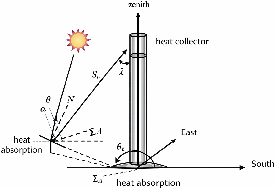
Figure 5: Cosine-efficiency geometry: incident ray, reflected ray, and mirror normal

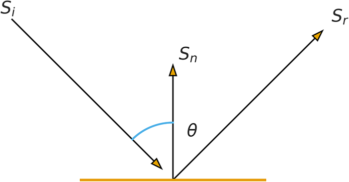
Figure 6: Cosine-efficiency geometry: incident ray Si, reflected ray Sr, mirror normal Sn, and incidence angle θ

Atmospheric transmittance.

For dHR≤1000m,

ηat=0.99321−1.17×10−4dHR+1.97×10−8dHR2.(11)

HFLCAL truncation.

Assume a circular Gaussian footprint on aperture ℛ:

ηtrunc=12πσtot2∬ℛexp(−x2+y2σtot2)dxdy,(12)

with

σtot2=d2(σsun2+σbq2+σast2+σtrack2),σbq=2σs, d=‖O−A‖.(13)

here σs denotes the mirror-slope error term, so that σbq=2σs collects the bi-axial slope contributions.

3.3 Objective, DNI, and Constraints

We adopt

DNI=G0[a+bexp(−csin⁡αs)],G0=1.366kW\,m−2.(14)

where a, b, and c are empirical clear-sky coefficients for the site, taken from [5]. Field output and per-area output are

Efield=DNI∑i=1NAiηi,E¯=Efield∑iAi.(15)

We maximize annual E¯ over ring radii {rj}, azimuthal spacings {Δθj}, mirror sizes li and heights hi subject to: base spacing ≥li+5 m; li∈[2,8] m; hi∈[2,6] m; collision-free rotations; rated annual output ≥60 MW. Frequently used symbols and geometric quantities are summarized in Table A1, Appendix A.

3.4 No-Occlusion Spacing and EB Prior

From the side-view construction (tower height Ht, base elevation Z0, ring radius Ri,j, receiver radius R0),

L1=(Ht−Z0)2+Ri,j2,α1=arcsin(Ri,jL1),α2=arcsin(R0L1),(16)

L3=tan⁡(α1+α2)(Ht−Z0),ΔRi,j=2(L3−Ri,j).(17)

Under an EB prior, ring-i azimuthal spacing grows outward. With scale Asf and spacing Ws,

ΔαZ,i=2arcsin(AsfWs2Ri,1),ΔAZi,j=2Ri,jsin(ΔαZ,i2),(18)

Nhel,i=⌊2πRi,jΔAZi,j⌋.(19)

4  Improved Cheetah Optimizer

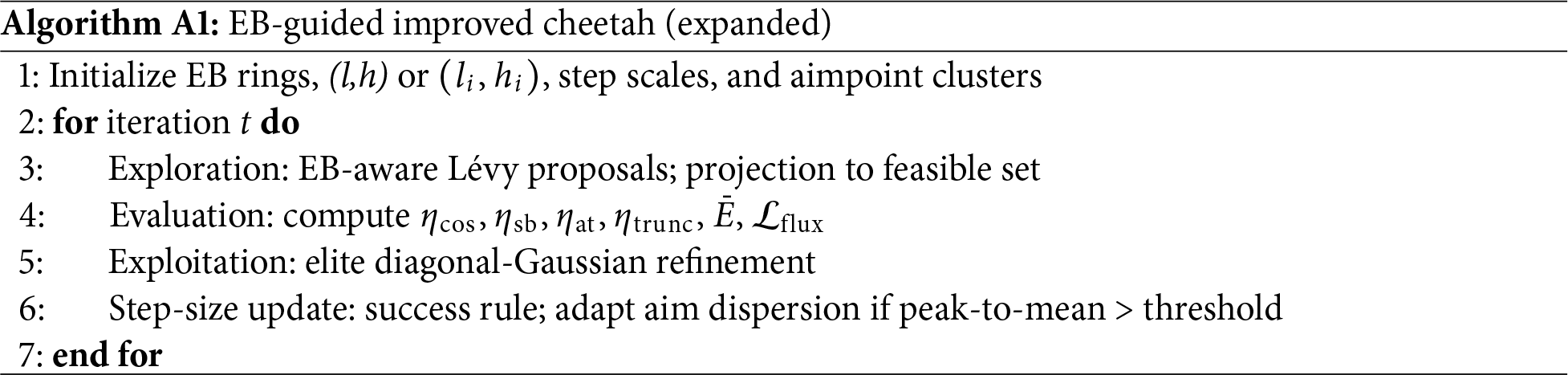
Our optimizer is structurally inspired by the coyote optimization algorithm [14], but we modify the step-generation and selection mechanisms and, for brevity, refer to this EB-guided variant as the “Cheetah” optimizer.

4.1 Decision Variables and EB-Guided Parameterization

Let the decision vector be

Θ=[r1,…,rI⏟ring radii,Δθ1,…,ΔθI⏟azimuthal spacings,l1,…,lN⏟mirror sizes,h1,…,hN⏟heights]⊤,

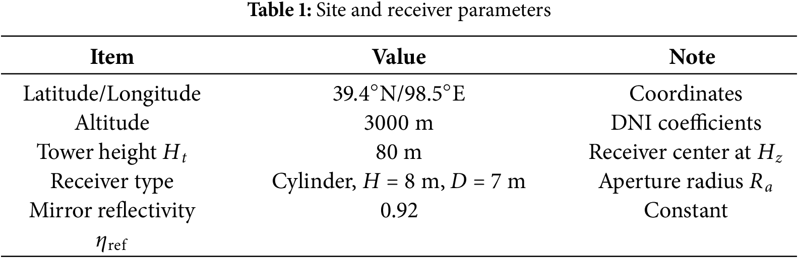
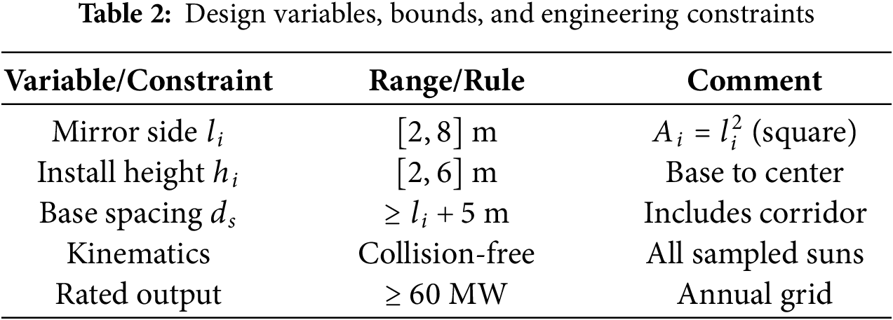
For the case study in Section 5, the site and receiver parameters are summarized in Table 1. The decision vector is subject to the engineering bounds summarized in Table 2, together with spacing/kinematics constraints and the rated-output requirement. To reduce search redundancy, we embed Θ on an EB-induced manifold derived from the Eliminate-Blocking radial-spacing rule used in SolarPILOT [9]: for ring i,

Δθi = 2arcsin(AsfWs2Ri,1),Nhel,i = ⌊2πRi2Risin⁡(Δθi/2)⌋,(20)

with global scalars (Asf,Ws) learned during search. This mapping captures the outward-growing azimuthal spacing of EB (Eliminate-Blocking) patterns; the resulting layouts are visualized in Section 6. It also empirically prunes low-quality packings before expensive optical evaluation [9,11].

4.2 Objective with Soft Constraints and Flux Cap

The optimizer maximizes annual per-area output E¯(Θ) under optical chain ηi=ηcos,iηsb,iηat,iηtrunc,iηref. We adopt stochastic ranking of a penalized score:

maxΘ∈ℱ J(Θ) = E¯(Θ) − ℒflux(Θ) − Ωhet(Θ) − 𝒫hard(Θ).(21)

Here ℒflux penalizes violations of panel-level peak-flux caps, Ωhet discourages excessive variation of heliostat size and height within a ring, and 𝒫hard collects residual violations of spacing and kinematic constraints. ℱ is the box-bounded hyper-rectangle and hard constraints (spacing, kinematics) are handled by projection and a residual penalty 𝒫hard. The panel flux cap uses a smooth softplus to limit peak flux on receiver panels p=1,…,P:

ℒflux(Θ)=λflux∑p=1Plog(1+exp((qp(Θ)−qpmax)/ε)).(22)

In (22), qp(Θ) is the predicted peak flux on receiver panel p from the HFLCAL footprint and panel clustering, qpmax is the admissible peak-flux limit for that panel, and ε is a small smoothing parameter (set to 0.05 in our experiments). qp(Θ) is peak flux predicted from HFLCAL footprint with clustered aimpoints per panel [9,15]; ε>0 sets smoothness. To discourage excessive size heterogeneity we add

Ωhet(Θ)=λℓ1∑i|li−lring(i)|+λh∑i|hi−hring(i)|.(23)

In (23), lring(i) and hring(i) denote the mean mirror side length and height within the ring that heliostat i belongs to. Promoting ring-wise size/height sharing for manufacturability and control simplicity.

4.3 Fast-Chase Exploration and Elite Refinement

We alternate two kernels:

(i) Cheetah “fast chase” exploration.

From each candidate Θ, propose an azimuth-aware Lévy-like step on the EB manifold:

Θ~ = Πℱ(Θ+DEBξα⏟Levy-like),ξα∼Stable(α,β=0,σ),(24)

where DEB scales radial components less than azimuthal ones to probe EB-consistent directions, α∈(1,2) controls tail-heaviness, σ is a per-block step scale, and Πℱ projects back to bounds [14]. This favors occasional large ring-level moves (escaping SB basins) while mostly sampling moderate within-ring refinements.

(ii) Elite-centered exploitation.

Elites {Θ(e)} spawn diagonal-Gaussian refinements

Θ^=Πℱ(Θ(e)+diag(σ)z),z∼𝒩(0,I),(25)

which stabilizes learning and keeps complexity linear in the dimension, unlike full-covariance CMA variants.

4.4 Success-Based Annealing and Restarts

Step scales σ follow a success rule:

σk+1={σkγ↑,if J(Θ~)≥J(Θ)σkγ↓,otherwise,γ↑>1>γ↓>0,(26)

applied per variable block (radii/azimuths/sizes/heights). If the best score stagnates for Tstall generations, a soft restart re-seeds part of the population around the current elite and part along random EB-consistent directions; if ring counts Nhel,i change (via Eq. (20)), the EB manifold is refreshed to keep feasibility (spacing, corridors) by local projection heuristics [11].

4.5 Feasibility Restoration and Stochastic Ranking

After each proposal we perform:

1.   Projection to bounds Πℱ;

2.   Spacing/kinematics repair: greedily increase ri or decrease li to meet ds≥li+5 m and avoid rotation collisions at sampled suns;

3.   Objective and penalties: evaluate E¯ and (22)–(23) from the optical chain;

4.   Stochastic ranking between score and constraint violation to maintain selection pressure near the feasible frontier.

Aiming uses panel clusters with dispersion tuned to HFLCAL variance, consistent with [9,15].

4.6 Algorithm and Complexity

Let M be the number of sampled sun positions per candidate. With neighbor pruning, SB cost is O(MNk) where k≪N is the average neighbor count (first rings). HFLCAL and attenuation are O(MN). The overall generation cost is linear in population size and dimension, enabling fair budget comparisons with GA/PSO/GWO [12,13] while preserving the stronger exploration of Lévy-like proposals [14].

4.7 Practical Notes and Baselines

The EB prior yields feasible seeds that respect outward-growing azimuthal spacing and corridor rules, reducing early wasted evaluations compared with uninformed GA/PSO/GWO [12,13]. The diagonal refinement keeps per-generation complexity linear and proved sufficient given the strong geometric prior; full covariance did not improve outcomes under equal budgets. In Section 6, we show that under the same evaluation budget the proposed scheme attains higher E¯ with lower variance, while meeting panel flux caps and rated output; qualitative layout differences are illustrated in Section 6.

5  Experimental Setup

Site/receiver. 98.5∘ E, 39.4∘ N, altitude 3000 m; tower 80 m; cylindrical receiver 8 m (height) × 7 m (diameter). ηref=0.92. The corresponding site and receiver parameters are summarized in Table 1.

Annual sampling. 21st of each month at 09:00, 10:30, 12:00, 13:30, 15:00 (Fig. 7 illustrates the angle/DNI trends) [20].

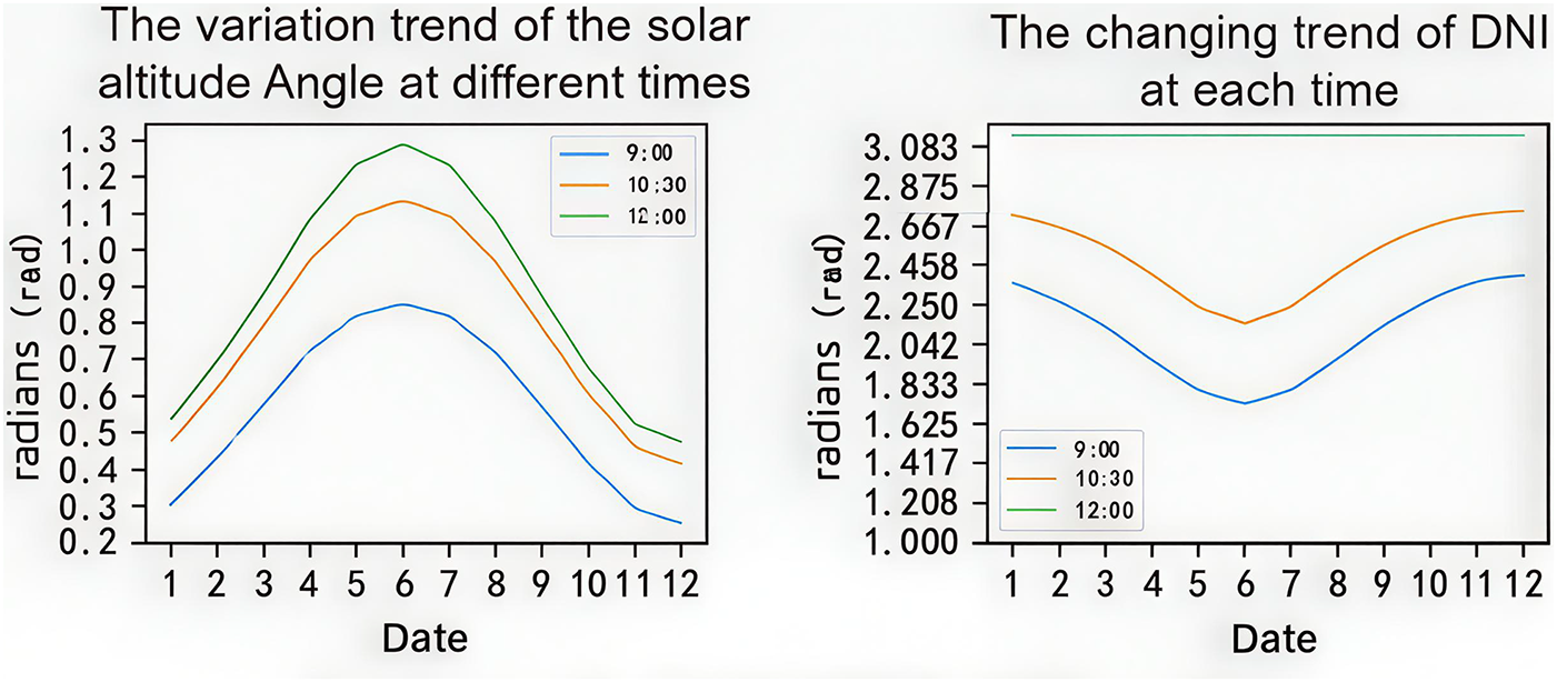
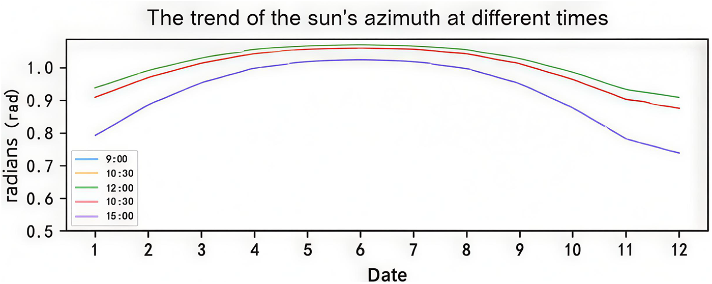
Figure 7: Illustrative annual trends: solar altitude/azimuth and DNI at sampled times

Design variables and constraints.

The design variables, bounds, and engineering constraints are summarized in Table 2.

6  Results and Discussion

6.1 Field Diagnostics and Spatial Distribution

Rings are near concentric with small intra-ring dispersion; spacing constraints are satisfied. Distribution-by-ring and selected inter-heliostat distances are reported in Tables 3 and 4, respectively; the spatial distribution is shown in Fig. 8.

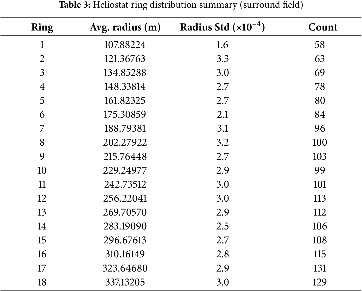
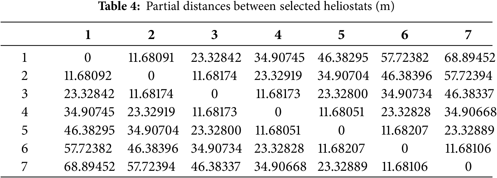
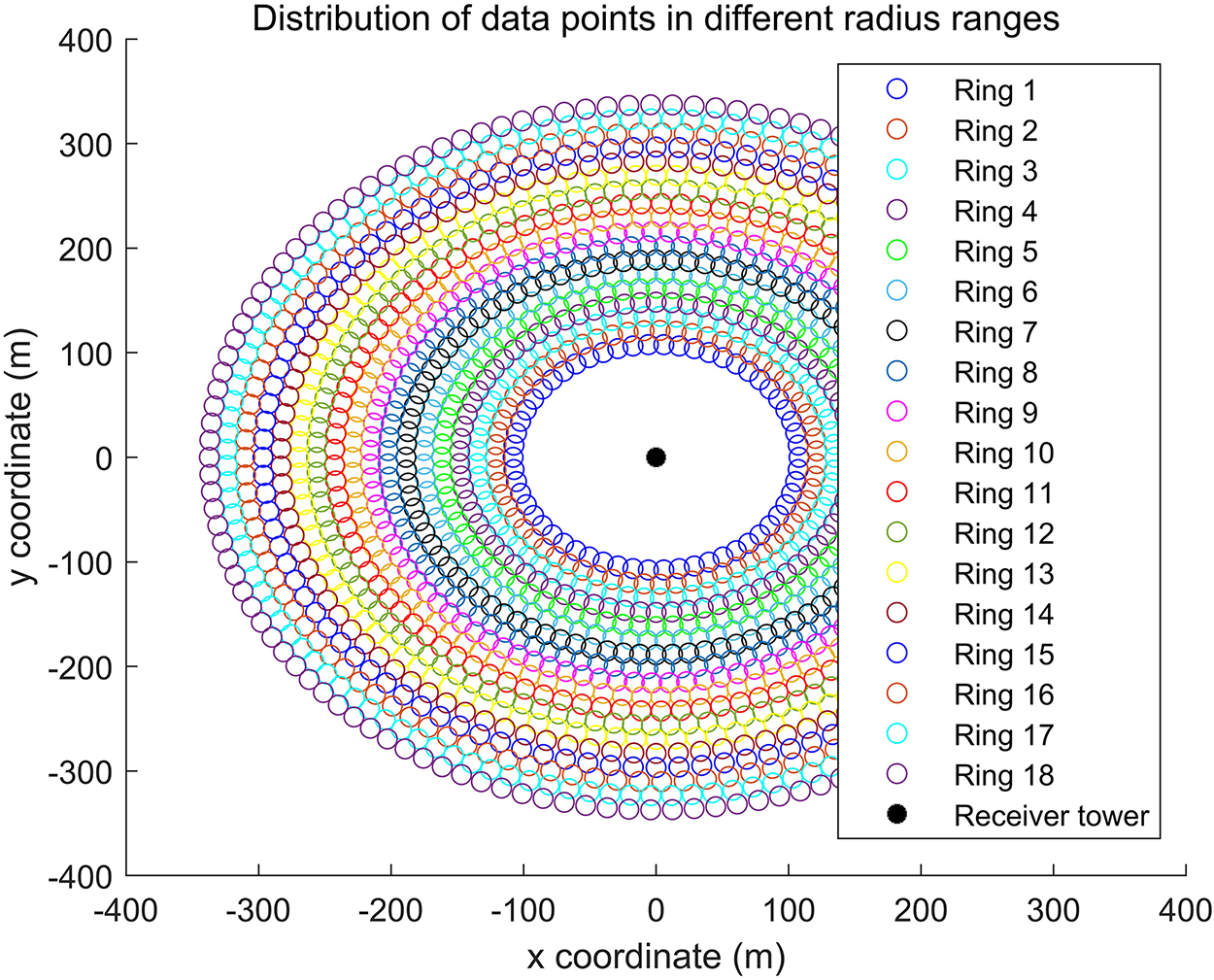
Figure 8: Distribution of heliostats by rings (data-point view)

6.2 Phase-Wise Gains and EB Layouts

The phase-wise outcomes under equal evaluation budgets are summarized in Table 5. From Phase I to Phase II, jointly tuning common size/height and ring parameters raises E¯ while meeting the rated target. Phase III further improves E¯ by assigning larger mirrors and higher installations where occlusions are weaker. EB layouts are illustrated in Figs. 9 and 10.

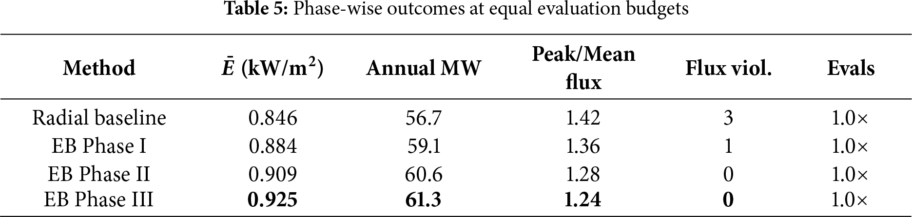
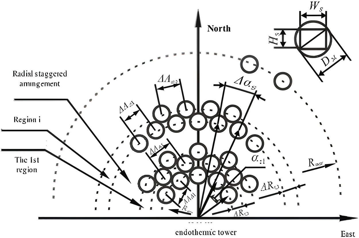
Figure 9: EB field layout diagram (surround-field view)

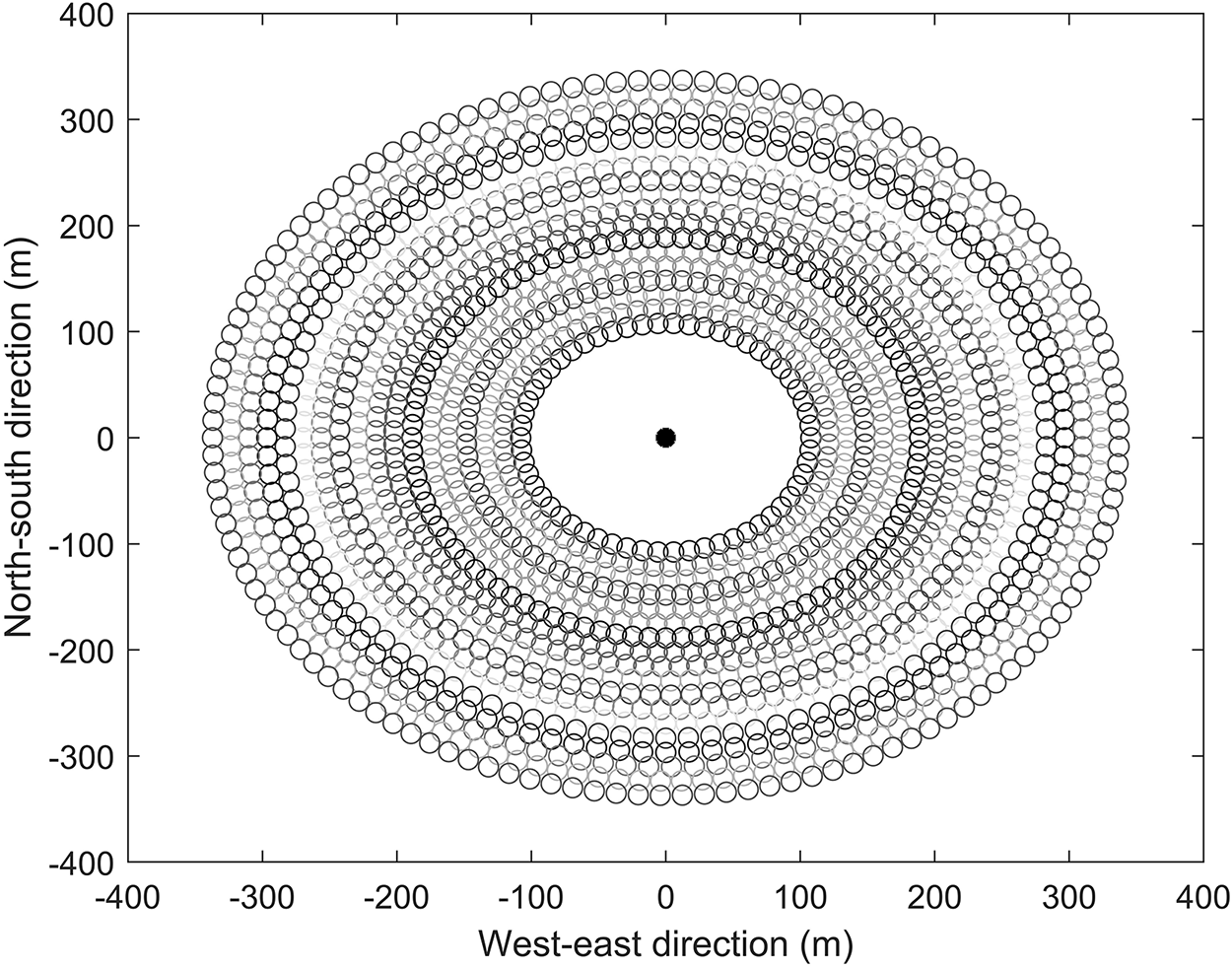
Figure 10: EB layout diagram (variant visualization for comparison)

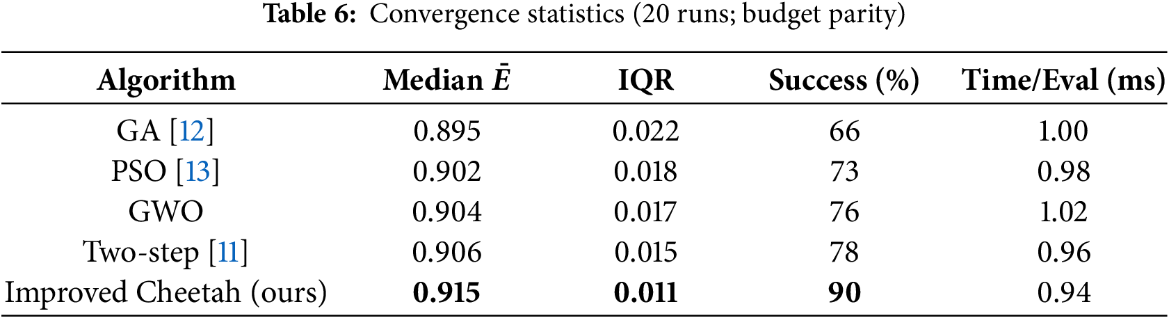
6.3 Algorithmic Convergence and Stability

Table 6 summarizes the convergence statistics over 20 runs under equal evaluation budgets.

6.4 Validation and Sensitivity

Projection-based SB (Figs. 3 and 4) tracks ray-tracing overlaps with small absolute errors in practical regimes (moderate incidence, nearest-neighbor occlusion) [6–8]. HFLCAL sensitivity follows the σtot composition; variations in σsun and σs dominate changes in ηtrunc, consistent with [3,4]. Under equal evaluations, the improved Cheetah converges faster with lower variance than GA/PSO/GWO [12–14], and EB spacing aligns with recent two-step insights [11].

6.5 Thermal Feasibility and Aiming Dispersion

Panel flux caps via ℒflux are respected across sampled suns; aiming dispersion reduces peak-to-mean by ∼10% relative to single-point aiming [9,15].

6.6 Uncertainty Quantification

Let ξ=[σsun,σs,σast,σtrack]⊤. First-order propagation on ηtrunc around ξ¯ gives

Var[ηtrunc]≈∇ξηtrunc⊤Σξ∇ξηtrunc,(27)

consistent with Monte Carlo estimates; Sobol indices rank σsun and σs as dominant.

7  Scalability and Cost-Aware Objective

Spatial indexing and cone filters reduce neighbor scans, giving near-linear scaling in N at fixed density. Cost proxy C(li,hi)=cmli2+cf+chhi and OPEX proxy co∑ili2 yield. For the cost-aware variant, we define

Jcost=E¯−α∑iC(li,hi)∑ili2−βco,(28)

promoting heterogeneity only where optical gains justify CAPEX [1].

8  Limitations and Future Work

We use representative clear-sky sampling; stochastic weather and soiling are not modeled. Extending to panel-level thermal models with stress-aware aiming and detailed O&M economics is a next step [15,17].

9  Conclusion

We presented a unified framework that integrates a validated projection loss model and HFLCAL truncation with an EB-guided improved Cheetah optimizer. Across three phases, the method improves annual per-area output relative to a radial baseline and reaches a 60 MW target with stable convergence. The workflow is auditable, modular, and adaptable to alternative receivers and sites, and is consistent with current reliability guidance and toolchains [8,9].

Acknowledgement: None.

Funding Statement: The authors received no specific funding for this study.

Author Contributions: Conceptualization, Zichang Meng and Hongfei Jiang; methodology, Zichang Meng; software, Zichang Meng; validation, Zichang Meng and Qi Li; formal analysis, Zichang Meng and Na Chen; investigation, Zichang Meng and Qi Li; resources, Hongfei Jiang; data curation, Zichang Meng; writing—original draft preparation, Zichang Meng; writing—review and editing, Na Chen, Qi Li, Qingyi Liu and Hongfei Jiang; visualization, Zichang Meng; supervision, Hongfei Jiang. All authors reviewed and approved the final version of the manuscript.

Availability of Data and Materials: The data and optimization scripts used in this study are available from the corresponding author upon reasonable request.

Ethics Approval: This study does not involve human participants or animal subjects, and no specific ethics approval was required.

Conflicts of Interest: The authors declare no conflicts of interest.

Appendix A: Notation

Appendix B: Closed-Form HFLCAL (Disk Aperture):

For a circular aperture of radius Ra and isotropic Gaussian footprint with variance σtot2,

ηtrunc=1−exp(−Ra2σtot2),(A1)

with sensitivities ∂ηtrunc/∂σtot and chain rules to component sigmas as in the main text.

Appendix C: Pseudocode

Appendix D: Neighbor Set Pruning:

A radial sweep with azimuthal gates and elevation cones yields a compact candidate set independent of N at fixed density. Only overlapping cones are tested for polygon intersection (consistent with two-step insights [2,11]).

References

1. Ho CK, Iverson BD. Advances in central receivers for concentrating solar power. Sol Energy. 2017;152:38–56. doi:10.1016/j.solener.2017.03.048. [Google Scholar] [CrossRef]

2. Noone CJ, Torrilhon M, Mitsos A. Heliostat field optimization: a new computationally efficient model and biomimetic layout. Sol Energy. 2012;86(2):792–803. doi:10.1016/j.solener.2011.12.007. [Google Scholar] [CrossRef]

3. Collado FJ, Guallar J. One-point fitting of the flux density produced by a heliostat. Sol Energy. 2010;84(4):673–84. doi:10.1016/j.solener.2010.01.019. [Google Scholar] [CrossRef]

4. Collado FJ, Guallar J. Campo: generation of regular heliostat fields. Renew Energy. 2012;46:49–59. doi:10.1016/j.renene.2012.03.011. [Google Scholar] [CrossRef]

5. Duffie JA, Beckman WA. Solar engineering of thermal processes. 4th edition. Hoboken, NJ, USA: John Wiley & Sons; 2013. [Google Scholar]

6. Wendelin T. SolTrace: a new optical modeling tool for concentrating solar optics. In: Proceedings of the ISEC 2003: International Solar Energy Conference; 2003 Mar 15–18; Kohala Coast, HI, USA. p. 253–60. [Google Scholar]

7. Smith DE, Hughes MD, Patel B, Borca-Tasciuc D-A. An open-source Monte Carlo ray-tracing simulation tool for luminescent solar concentrators with validation studies employing scattering phosphor films. Energies. 2021;14(2):455. doi:10.3390/en14020455. [Google Scholar] [CrossRef]

8. National Renewable Energy Laboratory (NREL). SolTrace: ray-tracing code for complex solar optical systems [internet]. [cited 2025 Nov 24]. Available from: https://www.nrel.gov/csp/soltrace-download.html. [Google Scholar]

9. Wagner MJ. SolarPILOT: a power tower solar field layout and characterization tool. Sol Energy. 2018;171:185–96. doi:10.1016/j.solener.2018.06.063. [Google Scholar] [CrossRef]

10. Ortega G, Rovira A. A new method for the selection of candidates for shading and blocking in central receiver systems. Renew Energy. 2020;152:961–73. doi:10.1016/j.renene.2020.01.130. [Google Scholar] [CrossRef]

11. Rizvi AA, Yang D, Khan TA. Optimization of biomimetic heliostat field using heuristic optimization algorithms. Knowl Based Syst. 2022;251:110048. doi:10.1016/j.knosys.2022.110048. [Google Scholar] [CrossRef]

12. Deb K, Pratap A, Agarwal S, Meyarivan T. A fast and elitist multiobjective genetic algorithm: NSGA-II. IEEE Trans Evol Comput. 2002;6(2):182–97. doi:10.1109/4235.996017. [Google Scholar] [CrossRef]

13. Kennedy J, Eberhart R. Particle swarm optimization. In: Proceedings of the IEEE International Conference on Neural Networks; 1995 Nov 27–Dec 1; Perth, WA, Australia. p. 1942–8. doi:10.1109/ICNN.1995.488968. [Google Scholar] [CrossRef]

14. Pierezan J, dos Santos Coelho L. Coyote optimization algorithm: a new metaheuristic for global optimization problems. In: Proceedings of the 2018 IEEE Congress on Evolutionary Computation (CEC); 2018 Jul 8–13; Rio de Janeiro, Brazil. p. 2633–40. doi:10.1109/CEC.2018.8477769. [Google Scholar] [CrossRef]

15. Wang K, He Y-L, Xue X-D, Du B-C. Multi-objective optimization of the aiming strategy for the solar power tower with a cavity receiver by using the non-dominated sorting genetic algorithm. Appl Energy. 2017;205:399–416. doi:10.1016/j.apenergy.2017.07.096. [Google Scholar] [CrossRef]

16. Sment J, Zolan A. Status quo and gap analysis of heliostat field deployment processes for concentrating solar tower plants. J Sol Energy Eng. 2024;146(6):061004. doi:10.1115/1.4065430. [Google Scholar] [CrossRef]

17. Zhu G, Augustine C, Mitchell R, Muller M, Kurup P, Zolan A, et al. Roadmap to advance heliostat technologies for concentrating solar-thermal power. Golden, CO, USA: National Renewable Energy Laboratory (NREL); 2022. Report No.: NREL/TP-5700-83041. doi: 10.2172/1888029. [Google Scholar] [CrossRef]

18. Xie X, Wang Y, Wang X, Zhang H. Optimization of heliostat field distribution based on an improved grey wolf optimizer. Renew Energy. 2021;176:447–58. doi:10.1016/j.renene.2021.05.058. [Google Scholar] [CrossRef]

19. Haris M, Rehman AU, Iqbal S, Athar SO, Kotb H, AboRas KM, et al. Genetic algorithm optimization of heliostat field layout for the design of a central receiver solar thermal power plant. Heliyon. 2023;9:e21488. doi:10.1016/j.heliyon.2023.e21488. [Google Scholar] [PubMed] [CrossRef]

20. Li C, Zhai R, Yang Y. Optimization of a heliostat field layout on annual basis using a hybrid algorithm combining particle swarm optimization algorithm and genetic algorithm. Energies. 2017;10(11):1924. doi:10.3390/en10111924. [Google Scholar] [CrossRef]