
 Login
Login Register
 Submit a Paper
 Propose a Special lssue
 Open Access
ARTICLE

A Fast Calculation Method for Dynamic Carbon Emission Factors Based on ILU Decomposition and BiCGSTABs
1 Metrology Center of Guangdong Power Grid Co., Ltd., Qingyuan, 511545, China
2 Dongguan Power Supply Bureau, Guangdong Power Grid Co., Ltd., Dongguan, 523129, China
3 Foshan Graduate School of Innovation, Northeastern University, Foshan, 528312, China
* Corresponding Author: Xiaoshun Zhang. Email:
(This article belongs to the Special Issue: Low-Carbon Situational Awareness and Dispatch Decision of New-Type Power System Operation)
Energy Engineering 2026, 123(6), 4 https://doi.org/10.32604/ee.2025.073240
Received 13 September 2025; Accepted 30 October 2025; Issue published 27 May 2026
 View Full Text
 Download PDF
Abstract
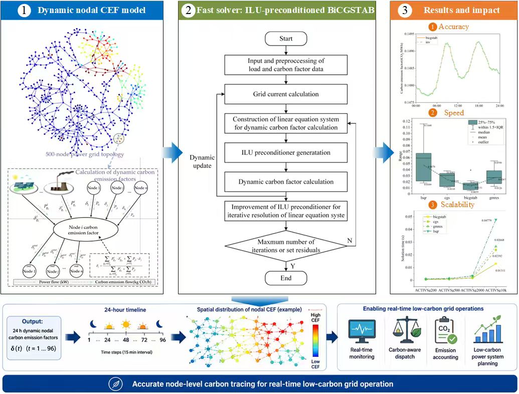
This paper addresses the challenge of efficiently calculating dynamic carbon emission factors (CEFs) in large-scale power systems. Traditional methods that rely on direct matrix inversion are computationally intensive and become impractical for networks with thousands of nodes. To overcome this limitation, a fast and scalable computational framework is proposed based on the incomplete LU (ILU) preconditioned biconjugate gradient stabilized (BiCGSTAB) iterative solver. The proposed approach formulates the nodal CEF model as a sparse linear system and employs Krylov subspace acceleration with ILU preconditioning to enhance convergence and numerical stability. The method is applied to synthetic power grid test cases ranging from 200 to 10,000 nodes to evaluate its accuracy and efficiency. Results show that the ILU-preconditioned BiCGSTAB algorithm achieves convergence within seven iterations, reducing computation time by more than two orders of magnitude compared with conventional direct matrix inversion. The method accurately tracks both local and imported carbon emissions at each node, providing fine-grained temporal and spatial emission profiles. Moreover, the ILU decomposition can be reused across time steps, further improving computational efficiency for dynamic and real-time scenarios. Overall, the proposed method demonstrates excellent scalability and robustness, making it well suited for high-frequency, real-time carbon emission monitoring in large power systems. The findings provide a computational foundation for carbon-aware dispatch, emission accounting, and policy-oriented applications in future low-carbon power grids.Graphic Abstract
Keywords
Under the national goals of “carbon peaking and carbon neutrality,” the power sector faces increasingly strict emission regulations. Traditional average carbon emission factors fail to capture regional and temporal differences, often underestimating actual emissions. In contrast, marginal or nodal emission factors offer more accurate and localized assessments. Carbon flow theory has recently been introduced to model emissions as a “virtual flow” that follows power flows, enabling emission traceability and the development of nodal carbon emission factor models. This helps reveal hidden disparities and supports region-specific decarbonization policies.
Based on this theory, several studies have proposed matrix-based models that calculate nodal emission factors through direct matrix inversion. Reference [1] calculated carbon emission flow in power systems using a matrix-based approach involving direct matrix inversion. While effective for small networks, this method faces computational challenges in large-scale applications. Reference [2] developed a carbon emission model for high-speed rail traction based on carbon flow theory and solved it via direct matrix inversion; however, this approach, while effective for localized applications, is computationally inefficient and difficult to scale to large power systems. Reference [3] calculated carbon emission factors for high-speed rail systems using carbon flow theory and direct matrix inversion. Reference [4] proposed a dynamic carbon emission factor model for distribution networks based on a generalized inverse matrix formulation. While their method enables accurate mapping between carbon factors and power flows, the reliance on matrix inversion limits scalability and computational efficiency in large-scale systems. Reference [5] developed a flow-based carbon accounting framework that computes nodal emission factors via linear system solutions. While accurate, the method relies on direct matrix operations, which may limit scalability in large power networks. Reference [6] computed nodal carbon emission factors by directly inverting the system allocation matrix in an improved carbon emission flow model. Although accurate, the method’s reliance on matrix inversion may limit its scalability under large-scale or real-time conditions.
The above studies have adopted matrix-based carbon flow models that compute nodal emission factors via direct matrix inversion. While accurate, these methods rely on dense linear algebra operations that are computationally expensive and difficult to scale. For a power system with an Jacobian matrix, the computational complexity of direct solvers can reach up to
Reference [7] proposed a parallel method for solving large-scale sparse state-space matrices in power systems, using incomplete LU decomposition with threshold pivoting (ILUTP) preconditioning combined with the biconjugate gradient stabilized (BiCGSTAB) iterative solver. This approach effectively reduces computational time and improves scalability in stability analysis applications. Reference [8] proposed a fast parallel solver for large sparse linear systems arising in bioluminescence tomography, based on preconditioned BiCGSTAB combined with CUDA. The method leverages incomplete Cholesky factorization and compressed row storage scheme (CSR) sparse matrix storage to enhance convergence and computational efficiency. Recent studies have investigated the application of iterative solvers in large-scale energy systems. Świrydowicz et al. [9] benchmarked several Krylov-based solvers for power grid optimization problems, highlighting their scalability in sparse grid matrices. Li et al. [10] demonstrated that a GPU-accelerated, preconditioned iterative solver significantly improves the efficiency of power flow analysis in large power systems. Qu et al. [11] further analyzed multigrid-preconditioned Krylov methods, confirming their effectiveness for non-symmetric and large-scale energy system models.
The above studies have successfully applied ILU-preconditioned BiCGSTAB algorithms to large-scale sparse systems in other fields. However, most existing CEF studies still rely on direct matrix inversion, which is simple and accurate for small systems but becomes inefficient for large-scale nodal networks. To date, no research has addressed this computational bottleneck or applied this approach to dynamic electric carbon emission factor calculations, where fast and scalable solutions are increasingly critical.
To address this gap, this paper introduces an ILU-preconditioned BiCGSTAB iterative algorithm to efficiently solve the nodal carbon emission factor model. BiCGSTAB is well-suited for nonsymmetric sparse systems, and the ILU preconditioner improves matrix conditioning to speed up convergence. While effective in other sparse problem domains, this method is applied here for the first time to carbon emission analysis. With proper parameter tuning, the approach ensures accuracy while significantly reducing computation time, making it suitable for real-time analysis in large-scale power grids. The main contributions are as follows:
• This paper adopts the BiCGSTAB iterative algorithm to efficiently solve nodal carbon emission factors in large-scale, nonsymmetric sparse systems. By leveraging Krylov subspace acceleration, the method achieves high precision with significantly lower computational cost than direct solvers, addressing the limitations of traditional approaches in large-scale and dynamic grid scenarios.
• An ILU preconditioner is integrated to improve numerical stability and convergence efficiency. By preserving matrix sparsity and enhancing conditioning, it reduces residual norms and supports repeated use in multi-period simulations, making the approach well-suited for real-time and time-series carbon emission analysis.
The novelty and contribution of this study lie in two main aspects. First, it is the first to employ an iterative-solver-based framework for large-scale dynamic carbon emission factor computation, overcoming the computational inefficiency of traditional matrix inversion. Second, compared with existing iterative methods such as CG, GMRES, and LSQR, the proposed ILU-preconditioned BiCGSTAB algorithm provides faster and more stable convergence for non-symmetric, sparse, and time-varying systems, offering clear advantages in both accuracy and scalability for real-time carbon emission analysis.
The remainder of this paper is organized as follows: Section 2 formulates the node-level dynamic CEF model, deriving the sparse linear system that captures carbon flow across power system nodes. Section 3 presents the fast computation framework based on the ILU-decomposed BiCGSTAB iterative solver, including analyses of matrix structure, preconditioning strategy, numerical efficiency, and its application to real-time carbon emission modeling. Section 4 provides a comprehensive case study using large-scale synthetic power grid datasets to validate the proposed method’s accuracy, scalability, and computational performance. Section 5 concludes the paper with a summary of key findings and a discussion of future research directions.
2 Calculation of Dynamic Carbon Emission Factors
In order to evaluate carbon emissions across nodes in a power system dynamically and efficiently, this work constructs a node-level carbon emission factor (CEF) model. The method accounts for both direct generation-side emissions and the imported carbon intensity from neighboring nodes through active power flow. The formulation is inherently recursive and reflects the coupling among all nodes within the network. Fig. 1 illustrates the overall modeling framework, including the grid topology and the flow-based CEF calculation logic.

Figure 1: Flow-based calculation of nodal carbon emission factors in a 500-node power grid
For a given node
where,
Eq. (1) captures the physical and environmental interactions at each node and forms the basis for further algebraic transformation. To facilitate a numerical solution for the entire network, Eq. (1) is algebraically rearranged into the following linear form:
By applying this equation to all nodes in the system, we derive a sparse linear algebraic system in the compact form:
In this equation,
The structure of Eq. (3) reflects both the network topology and the real-time power flow distribution, forming a consistent and physically interpretable representation of carbon emission propagation across the grid.
To quantify numerical difficulty and its impact on Krylov convergence, we evaluate the condition number

Figure 2: Condition number of the sparse coefficient matrix A vs. matrix dimension across four test systems
These values increase with system size, reflecting the growing challenge of the unpreconditioned problem. With an ILU preconditioner
To improve readability of the mathematical formulations in Eqs. (1)–(3), the key variables and parameters are summarized in Table 1, which lists their definitions and corresponding units.

3 Fast CEF Computation Based on ILU-Decomposed BiCGSTAB Solver
As previously established in Eq. (3), the dynamic CEF at each node is computed by solving a sparse linear system. Given that Eq. (3) must be solved repeatedly across multiple time intervals, the efficiency of the solver is critical. Direct inversion, though accurate, has computational complexity on the order of
3.1 Structure and Sparsity of the System Matrix
The matrix
The right-hand side vector
This structure leads to a matrix with a relatively small average number of nonzero entries per row—commonly denoted as
3.2 Preconditioned BiCGSTAB Framework
BiCGSTAB is used to solve
where
with a target tolerance
To improve convergence, we introduce a left preconditioner
where,
with
During preconditioning, the residual update step becomes:
and all matrix-vector products in the BiCGSTAB loop are replaced with operations involving
To clearly illustrate the computational structure of the proposed preconditioned iterative solver for dynamic CEF estimation, the workflow is summarized in Fig. 3. The process begins with the input and preprocessing of load and carbon factor data, followed by grid current calculations and the formation of a sparse linear equation system. An ILU preconditioner is then generated and further improved to enhance convergence efficiency. The solver computes the dynamic carbon factor iteratively and checks convergence at each step. Convergence is determined by either reaching the maximum number of iterations or satisfying a predefined residual threshold. If convergence is not reached, the solver performs dynamic updates to refine the grid currents and ILU preconditioner for the next iteration cycle.

Figure 3: Iterative workflow of ILU-preconditioned BiCGSTAB for dynamic carbon factor computation
3.3 Numerical Efficiency and Reusability
A key advantage of BiCGSTAB with ILU(0) is the reusability of the ILU decomposition
Furthermore, the average iteration count for convergence is empirically bounded:
which implies a total complexity of:
per solve. Compared to the
The computational complexity of the proposed ILU-preconditioned BiCGSTAB solver per iteration is approximately
3.4 Application to Carbon Emission Modeling
The solution
Nodal emissions:
Branch losses:
Total daily emissions:
Thus, the proposed method forms the computational backbone for fast, high-resolution carbon emission analysis across a wide range of power system scenarios.
To verify the accuracy and computational efficiency of the proposed BiCGSTAB method with ILU preconditioning for CEF calculations, we conducted a series of numerical experiments based on publicly available synthetic power system cases developed by Texas A&M University. These cases, known as ACTIVSg, represent power grids of varying sizes and structural complexity, designed to mimic the statistical and operational characteristics of real-world systems without exposing confidential data.
Specifically, four test cases were selected: ACTIVSg200 (approximately 200 buses), ACTIVSg500 (500 buses), ACTIVSg2000 (2000 buses), and ACTIVSg10k (10,000 buses). These systems simulate the regional grids of Central Illinois, South Carolina, Texas, and the Western United States, respectively. Each system features distinct levels of complexity in terms of topology, voltage levels, and area partitioning, ranging from a single-zone, three-voltage network to a 16-zone, multi-voltage structure including 500 kV down to 13.2 kV.
Table 2 summarizes the basic characteristics of these four test cases, including the number of buses, loads, generators, and branch lines, as well as voltage levels and simulated geographical areas.

The test systems also incorporate diverse energy portfolios with varying carbon intensities. For instance, the ACTIVSg10k model includes 2485 generators using coal, natural gas, nuclear, hydro, wind, and solar energy. The average carbon emission factors for these energy types range from 0.0382 to 0.7175

Based on the above settings, we calculated the total daily carbon emissions for each system using the BiCGSTAB method. These simulations span 96 time steps (every 15 min over 24 h), covering both nodal injection losses and branch transmission losses. Table 4 reports the results.

To validate the numerical accuracy of the proposed BiCGSTAB algorithm with ILU preconditioning, a comparison was conducted against the direct matrix inversion (inv) method. As shown in Fig. 4, the carbon emission factor curves calculated by both methods over a 24-h period exhibit an exact match, demonstrating that the iterative solver achieves high numerical accuracy consistent with the direct solution. The results confirm that BiCGSTAB is suitable for reliable CEF estimation in power system applications.

Figure 4: Comparison of carbon emission factor calculated by BiCGSTAB and matrix inversion methods over 24 h
Using the BiCGSTAB method, we further computed the total carbon emissions of the ACTIVSg200 system over a full day (96 time intervals). The result, illustrated in Fig. 5, shows the temporal variation of aggregate emissions measured in tons of

Figure 5: Total carbon emissions calculated by BiCGSTAB in the ACTIVSg200 system over 24 h
To further evaluate the efficiency and robustness of the proposed BiCGSTAB algorithm on large-scale systems, we performed comparative experiments using the ACTIVSg10k case, which contains 10,000 buses and over 12,000 branches. Four commonly used iterative solvers were selected for comparison: least squares QR (LSQR), conjugate gradient squared (CGS), BiCGSTAB, and generalized minimum residual (GMRES).
We standardize solver parameters to ensure a fair comparison across methods. All iterative solvers terminate when the relative residual

Figure 6: Convergence accuracy of BiCGSTAB, CGS, GMRES, and LSQR over 9 iterations on the ACTIVSg10k system. BiCGSTAB converges fastest to high precision
To assess time stability across multiple trials, Fig. 7 shows a boxplot comparing the execution time range of the four iterative methods over repeated runs on the 10k system. BiCGSTAB not only exhibits the lowest average runtime but also the narrowest variance, indicating both high computational speed and consistency. In contrast, LSQR shows the largest variability and longest tail, suggesting it is less reliable under large-scale sparse matrix conditions.

Figure 7: Runtime statistics of iterative solvers (boxplot). BiCGSTAB shows the lowest average runtime and best stability among all methods
To evaluate solver scalability, Fig. 8 compares the solution time of each method as system size increases. All solvers show rising computation time with larger grids, but BiCGSTAB grows the slowest, maintaining the shortest runtime across all cases. In contrast, LSQR scales poorly, with its time increasing steeply in the 10k case. This confirms that BiCGSTAB offers not only accuracy and stability but also excellent scalability for large-scale applications.

Figure 8: Solver runtime vs. system size. BiCGSTAB shows the best scalability performance
In order to quantitatively illustrate the performance trends observed in Figs. 6–9, detailed numerical results are summarized in Tables 5 and 6. Table 5 lists the convergence accuracy evolution of each iterative solver across nine iterations, while Table 6 reports the computation time of the proposed ILU-preconditioned BiCGSTAB and other solvers under different power grid scales. These tables provide clear numerical evidence supporting the observed trends in convergence, stability, and scalability.

Figure 9: Computation-time benefits of ILU preconditioner reuse in dynamic ECF. (a) Total time across four systems; (b) Speedup due to reuse (with/without first build); (c) Time breakdown over 96 periods (case_ACTIVSg200); (d) Time saving percentage across systems


As shown in Table 5, the ILU-preconditioned BiCGSTAB solver exhibits a monotonic residual reduction from
As shown in Fig. 9, we compare two strategies across 96 time periods for four benchmark systems (200, 500, 2000, and 10k buses): (i) re-factorization at every time step and (ii) reuse of the ILU factors computed at the first time step. For completeness, two reuse scenarios are reported: Strategy-1 includes the one-off initial factorization cost; Strategy-2 excludes it (ideal reuse). Totals over 96 periods are as follows:
• case_ACTIVSg200: re-factorization 0.065844 s; reuse-1 0.059550 s (9.56% saving;
• case_ACTIVSg500: re-factorization 0.077042 s; reuse-1 0.066552 s (13.62% saving;
• case_ACTIVSg2000: re-factorization 0.167054 s; reuse-1 0.122449 s (26.70% saving;
• case_ACTIVSg10k: re-factorization 1.231801 s; reuse-1 1.095325 s (11.08% saving;
The data show consistent time savings (
It is worth noting that the direct inverse method is not shown in the boxplot because its execution time was prohibitively long—averaging around 8 s per solve, which makes it impractical for large-scale dynamic carbon emission analysis.
Beyond the computational performance demonstrated above, the proposed ILU-preconditioned BiCGSTAB framework enables real-time and high-resolution CEF estimation even in large-scale nodal systems, which is essential for practical carbon management and policy applications. The ability to compute accurate emission factors across thousands of nodes within seconds allows system operators and regulators to track carbon flows dynamically and make timely, data-driven decisions. Such fast and scalable CEF calculations can significantly enhance regional emission accounting accuracy, support carbon pricing and emission trading mechanisms, and facilitate low-carbon dispatch and planning strategies in power systems of increasing complexity. These broader applications will be further explored in future studies integrating the proposed computational method with carbon policy and operational decision models.
This paper presents a fast and scalable method for calculating dynamic carbon emission factors (CEFs) in large-scale power systems using the ILU-preconditioned BiCGSTAB iterative solver. The proposed method effectively overcomes the computational limitations of traditional matrix inversion techniques, achieving significant improvements in both efficiency and scalability. Numerical results show that the BiCGSTAB solver with ILU preconditioning provides accurate and rapid CEF calculations, making it suitable for real-time carbon emission analysis in large power grids.
Compared with conventional direct solvers, the proposed approach achieves faster convergence and lower computational costs, particularly in dynamic grid scenarios involving multiple time intervals and large-scale systems. This work contributes to the field by introducing an efficient iterative framework for calculating dynamic CEFs, which can be applied to various power system configurations and support carbon emission monitoring and reduction strategies.
The case studies are based on synthetic ACTIVSg test systems, which accurately represent the structural and operational characteristics of real power grids. However, real-world data may contain measurement noise and missing information that could affect model accuracy. This limitation will be addressed in future work to enhance the robustness of the proposed method under practical operating conditions.
It should also be noted that the performance of the algorithm can be sensitive to the choice of preconditioner parameters. Future studies will explore adaptive or optimized preconditioning strategies to improve convergence stability under different grid conditions. Furthermore, future research will focus on integrating the proposed CEF model with renewable energy forecasting and real-time dispatch frameworks to support carbon-aware grid operations. The method may also be extended to multi-energy systems to analyze interactive carbon flows among electricity, heat, and gas networks, thereby strengthening its role in low-carbon system planning and operation.
Acknowledgement: Not applicable.
Funding Statement: This work was supported by the Science and Technology Project of China Southern Power Grid Co., Ltd. (031900KC24040022 (GDKJXM20240391)).
Author Contributions: The authors confirm contribution to the paper as follows: Conceptualization, Lihua Zhong and Xiaoshun Zhang; methodology, Lihua Zhong; validation, Lihua Zhong, Feng Pan and Yuyao Yang; formal analysis, Lihua Zhong; resources, Lei Feng and Jinghe Jiang; data curation, Guo Lin; writing—original draft preparation, Lihua Zhong; writing—review and editing, Lihua Zhong; visualization, Yuyao Yang; supervision, Xiaoshun Zhang. All authors reviewed the results and approved the final version of the manuscript.
Availability of Data and Materials: The data presented in this study are available on request from the corresponding author.
Ethics Approval: Not applicable.
Conflicts of Interest: The authors declare no conflicts of interest to report regarding the present study.
Abbreviations
| CEF | Carbon emissionfactors |
| ILU | Incomplete LU |
| BiCGSTAB | Biconjugate gradient stabilized |
References
1. Cheng Y, Zhang N, Kang C. Carbon emission flow: from electricity network to multiple energy systems. Global Energy Interconnect. 2018;1(4):500–6. doi:10.14171/j.2096-5117.gei.2018.04.010. [Google Scholar] [CrossRef]
2. Song J, Chen X, Lu C, Shi X, Yan Y, Zhang S. High-speed rail electric traction carbon emission calculation method based on carbon flow theory. IEEE Access. 2024;12:102096–110. doi:10.1109/access.2024.3425911. [Google Scholar] [CrossRef]
3. Wang Y, Qiu J, Tao Y, Zhao J. Carbon-oriented operational planning in coupled electricity and emission trading markets. IEEE Trans Power Syst. 2020;35(4):3145–57. doi:10.1109/tpwrs.2020.2966663. [Google Scholar] [CrossRef]
4. Zhang X, Guo Z, Pan F, Yang Y, Li C. Dynamic carbon emission factor based interactive control of distribution network by a generalized regression neural network assisted optimization. Energy. 2023;283:129132. doi:10.1016/j.energy.2023.129132. [Google Scholar] [CrossRef]
5. Chen X, Chao H, Shi W, Li N. Towards carbon-free electricity: a flow-based framework for power grid carbon accounting and decarbonization. arXiv:2308.03268. 2023. [Google Scholar]
6. Zhu X, Liu Z, Shen R, Wang Q, Tang A, You X, et al. Research on an improved carbon emission flow model considering electric vehicle charging fluctuation and hybrid power transaction. Energies. 2023;16(19):6835. doi:10.3390/en16196835. [Google Scholar] [CrossRef]
7. Wang K, Ye M, Liu Y. Parallel method for establishing the state-space equations of power systems. J Zhengzhou Univ (Eng Sci Edit). 2021;42(1):15–20. (In Chinese). [Google Scholar]
8. Feng J, Li Y, Li Z, Jia K. BLT fast parallel forward method combining preconditioned BiCGStab and CUDA. J Beijing Univ Technol. 2017;43(11):1658–65. (In Chinese). [Google Scholar]
9. Świrydowicz K, Darve E, Jones W, Maack J, Regev S, Saunders MA, et al. Linear solvers for power grid optimization problems: a review of GPU-accelerated linear solvers. Parallel Comput. 2022;111(1):102870. doi:10.1016/j.parco.2021.102870. [Google Scholar] [CrossRef]
10. Li X, Li F, Yuan H, Cui H, Hu Q. GPU-based fast decoupled power flow with preconditioned iterative solver and inexact newton method. IEEE Trans Power Syst. 2017;32(4):2695–703. doi:10.1109/pesgm.2017.8274624. [Google Scholar] [CrossRef]
11. Qu Y, Aage N, Li Q. On the effectiveness of multigrid preconditioned iterative methods for large-scale frequency response topology optimization problems. Adv Eng Softw. 2025;210:104017. doi:10.1016/j.advengsoft.2025.104017. [Google Scholar] [CrossRef]
12. Liu Z, Guan D, Wei W, Davis SJ, Ciais P, Bai J, et al. Reduced carbon emission estimates from fossil fuel combustion and cement production in China. Nature. 2015;524(7565):335–8. doi:10.1038/nature14677. [Google Scholar] [PubMed] [CrossRef]
13. Shan Y, Liu J, Liu Z, Xu X, Shao S, Wang P, et al. New provincial CO2 emission inventories in China based on apparent energy consumption data and updated emission factors. Appl Energy. 2016;184:742–50. doi:10.1016/j.apenergy.2016.03.073. [Google Scholar] [CrossRef]
14. Wang L, Wang Y, Du H, Zuo J, Li R, Zhou Z, et al. A comparative life-cycle assessment of hydro-, nuclear and wind power: a China study. Appl Energy. 2019;249:37–45. doi:10.1016/j.apenergy.2019.04.099. [Google Scholar] [CrossRef]
15. Varun, Prakash R, Bhat IK. Life cycle greenhouse gas emissions estimation for small hydropower schemes in India. Energy. 2012;44(1):498–508. doi:10.1016/j.energy.2012.05.052. [Google Scholar] [CrossRef]
16. Gemechu E, Kumar A. A review of how life cycle assessment has been used to assess the environmental impacts of hydropower energy. Renew Sustain Energ Rev. 2022;167:112684. doi:10.1016/j.rser.2022.112684. [Google Scholar] [CrossRef]
17. Ludin NA, Mustafa NI, Hanafiah MM, Ibrahim MA, Asri Mat Teridi M, Sepeai S, et al. Prospects of life cycle assessment of renewable energy from solar photovoltaic technologies: a review. Renew Sustain Energy Rev. 2018;96:11–28. doi:10.1016/j.rser.2018.07.048. [Google Scholar] [CrossRef]
18. Rahman A, Farrok O, Haque MM. Environmental impact of renewable energy source based electrical power plants: solar, wind, hydroelectric, biomass, geothermal, tidal, ocean, and osmotic. Renew Sustain Energ Rev. 2022;161:112279. doi:10.1016/j.rser.2022.112279. [Google Scholar] [CrossRef]
19. Proops JL, Gay PW, Speck S, Schroder T. The lifetime pollution implications of various types of electricity generation. An input-output analysis. Energy Policy. 1996;24(3):229–37. doi:10.1016/0301-4215(95)00154-9. [Google Scholar] [CrossRef]
20. Hondo H. Life cycle GHG emission analysis of power generation systems: Japanese case. Energy. 2005;30(11–12):2042–56. doi:10.1016/j.energy.2004.07.020. [Google Scholar] [CrossRef]
21. Amponsah NY, Troldborg M, Kington B, Aalders I, Hough RL. Greenhouse gas emissions from renewable energy sources: a review of lifecycle considerations. Renew Sustain Energy Rev. 2014;39(1):461–75. doi:10.1016/j.rser.2014.07.087. [Google Scholar] [CrossRef]
22. Saini P, Singh S, Kajal P, Dhar A, Khot N, Mohamed ME, et al. A review of the techno-economic potential and environmental impact analysis through life cycle assessment of parabolic trough collector towards the contribution of sustainable energy. Heliyon. 2023;9(7):e17626. doi:10.1016/j.heliyon.2023.e17626. [Google Scholar] [PubMed] [CrossRef]
23. Lenzen M. Life cycle energy and greenhouse gas emissions of nuclear energy: a review. Energy Conver Manag. 2008;49(8):2178–99. doi:10.1016/j.enconman.2008.01.033. [Google Scholar] [CrossRef]
Cite This Article
 Copyright © 2026 The Author(s). Published by Tech Science Press.
This work is licensed under a Creative Commons Attribution 4.0 International License , which permits unrestricted use, distribution, and reproduction in any medium, provided the original work is properly cited.
 Downloads
 Citation Tools
