
 Login
Login Register
 Submit a Paper
 Propose a Special lssue
 Open Access
ARTICLE

A Novel Comparative Analysis of Statistical and Deep Learning Approaches for Time Series Forecasting of Solar Energy Output
1 Laboratory of Intelligent Systems, Advanced Mechanics and Renewable Energy, Faculty of Sciences and Technology, Sultan Moulay Slimane University, Beni Mellal, Morocco
2 Laboratory MIET, Faculty of Sciences and Technology, Hassan 1st University, Settat, Morocco
* Corresponding Author: Said Benkachcha. Email:
(This article belongs to the Special Issue: Advances and Emerging Trends in Photovoltaic Technologies, Energy Storage, and Green Hydrogen)
Energy Engineering 2026, 123(6), 6 https://doi.org/10.32604/ee.2026.075406
Received 31 October 2025; Accepted 04 January 2026; Issue published 27 May 2026
 View Full Text
 Download PDF
Abstract
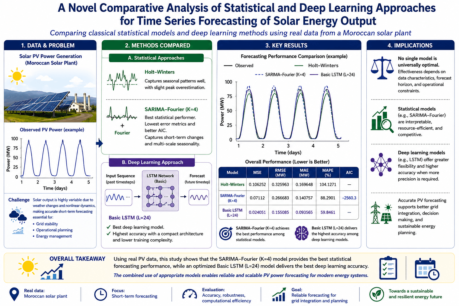
Accurate forecasting of solar photovoltaic (PV) power generation is essential for enabling reliable integration of renewable energy into modern power systems. Variability in solar production, driven by meteorological fluctuations and inherent nonlinear dynamics, presents significant challenges for grid stability, operational planning, and energy management. This study investigates and compares the performance of classical statistical forecasting techniques and advanced deep learning approaches using real PV production data from a Moroccan solar plant. The analysis focuses on accuracy, robustness, computational efficiency, and suitability for short-term operational applications. Among statistical approaches, the Holt–Winters model demonstrated strong capability in reproducing seasonal patterns, although it exhibited slight peak overestimation. The Seasonal ARIMA (SARIMA) model enhanced with Fourier terms provided the best statistical performance, achieving the lowest error metrics and an improved Akaike Information Criterion (AIC), confirming its ability to jointly capture short-term variations and multi-scale seasonality. In contrast, deep learning models offered superior representational flexibility but required higher computational cost and careful tuning. The Basic LSTM architecture, after sequence-length optimization, outperformed other neural models by delivering high predictive accuracy with a compact network structure and reduced training complexity. The results highlight that no single model is universally optimal; instead, forecasting effectiveness depends on data characteristics, horizon requirements, and operational constraints. Statistical models remain competitive for interpretable and resource-efficient applications, whereas neural models are advantageous when higher predictive precision is required. Overall, the findings contribute to the development of reliable and scalable PV forecasting strategies, supporting improved grid integration, enhanced decision making, and sustainable energy planning.Graphic Abstract
Keywords
The global energy sector is shifting toward renewable sources to combat climate change, with solar energy emerging as a promising solution [1]. Photovoltaic energy has the potential to produce clean, sustainable electricity and significantly reduce greenhouse gas (GHG) emissions. However, integrating solar power into electrical grids poses unique challenges due to the inherent variability and unpredictability of solar output. To maintain grid stability and optimize energy scheduling, accurate photovoltaic (PV) power forecasting is essential [2,3].
The energy industry’s commitment to reducing carbon emissions has accelerated the transition from fossil fuels—like coal, natural gas, and petroleum—that contributes to GHG emissions and environmental degradation. As industrialization increases energy demand, fossil fuel reserves are under pressure, reinforcing the need for renewable alternatives. Solar power is a key renewable resource, able to generate significant electricity without depleting non renewable reserves. Integrating solar energy into the grid provides environmental and economic advantages, such as lowered GHG emissions and reduced energy production costs [4,5].
Effective forecasting of renewable energy generation is essential for optimizing grid operations across various sources, including solar, wind, and hydroelectric power. By accurately predicting energy production, forecasting helps balance supply and demand, ensuring reliable integration of these resources into the power system [6]. In particular, solar PV forecasting plays a crucial role by reducing uncertainties in energy output, which is vital for the efficient and cost-effective management of renewable resources [7].
Nevertheless, integrating PV power into the grid remains challenging due to its variability. The rapid expansion of PV capacity has introduced new complexities in maintaining grid stability and reliability [8]. PV systems provide environmental benefits and are simpler to operate than fossil fuel plants, they face issues related to intermittency and output fluctuations. These variations can disrupt the balance between energy generation and consumption, risking grid stability. Therefore, accurate PV power forecasting is essential for addressing these challenges and stands as one of the most effective and economical strategies for ensuring a stable, efficient, and resilient energy supply [9].
Effective PV solar forecasting facilitates the integration of renewable energy at various scales, enhances grid management, supports peak shaving, and reduces overall operational costs. Accurate forecasts enable optimal energy scheduling, improved storage management, and help minimize financial losses caused by the under- or over-utilization of power systems [10]. PV solar forecasting approaches are classified based on two main factors: the forecast horizon and the forecasting method. The forecast horizon represents the time gap between the current moment and the prediction period [11,12], while the forecasting method determines the model’s ability to achieve accurate predictions. Addressing both factors improves the accuracy and applicability of PV power forecasts.
In the literature, PV solar forecasting techniques are commonly grouped according to their modelling philosophy and data requirements. These include physical methods, statistical approaches, machine learning techniques, deep learning models, and hybrid frameworks that combine multiple strategies to enhance prediction reliability.
Physical Methods: Physical methods rely on meteorological data, such as solar radiation, temperature, and cloud cover, to predict solar energy production. Techniques like Numerical Weather Prediction (NWP) and cloud imaging utilize physical models to estimate solar irradiance, which is then converted into expected PV power output. Physical methods are effective for forecasting when detailed weather data is available, as they capture external environmental factors influencing solar energy.
Statistical Methods: Statistical methods leverage historical data to uncover relationships between input variables (like weather data) and solar power output. Common models include Autoregressive (AR), Autoregressive Moving Average (ARMA), and Autoregressive Integrated Moving Average (ARIMA). Additionally, linear regression, support vector regression (SVR), and Markov chains are widely used [13]. While statistical methods are valuable for simpler data patterns, they often assume linearity, which may limit their effectiveness in capturing the complex dynamics of solar data.
Machine Learning (ML) Methods: ML methods excel in identifying complex patterns within large datasets without assuming predefined data structures. Techniques such as decision trees, random forests, and gradient boosting are particularly useful for handling non-linear relationships in data. ML models are highly effective for short-term forecasting, where fast predictions are necessary to support grid integration and operational decisions [14].
Deep Learning (DL) Methods: DL methods, a subset of ML, employ neural networks to model non-linear relationships in data. Models like Feedforward Neural Networks (FFNN), Recurrent Neural Networks (RNN), and Long Short-Term Memory (LSTM) networks are highly effective for time-dependent data, making them ideal for long-term solar forecasting. By capturing sequential dependencies, DL methods can model the complex and evolving patterns in solar power generation [15,16].
Hybrid Methods: Hybrid methods combine multiple forecasting approaches, often integrating physical and statistical methods or blending ML and DL models [17]. These methods aim to capture both short-term variability and long-term trends in PV power production [18]. For instance, combining physical models with ML techniques can enhance forecast accuracy by leveraging weather data and data-driven insights, providing a more comprehensive view of PV output.
In a 2023 study, Scott et al. [19] performed an in-depth analysis of forecasting methods across various time horizons and dataset sizes. The study aimed to assess different machine learning algorithms (MLAs) for predicting photovoltaic (PV) output at a university campus in central Manchester, England. Four MLA models—random forest (RF), neural networks (NN), support vector machines (SVM), and linear regression (LR)—were developed and validated using real-time data. The results revealed that RF achieved the lowest average root mean squared error (RMSE) of 32, outperforming SVM, LR, and NN, which recorded RMSE values of 32.3, 36.5, and 38.9, respectively.
Liu et al. [20] utilized a SCADA database to analyse offshore wind speeds collected from a measuring tower in Scotland over the course of 2018. They employed the Seasonal Auto-Regression Integrated Moving Average (SARIMA) method to forecast short-term wind speeds, assessing model performance through metrics such as R-square, Explained Variance Score, and Mean Absolute Error. The results indicated that the SARIMA model outperformed deep learning algorithms like Gated Recurrent Unit (GRU) and Long Short-Term Memory (LSTM), suggesting that traditional statistical methods may be more effective for short-term forecasting in this context.
de C Costa [21] utilized real-world data to predict photovoltaic power generation using various methods, including LSTM, Convolutional, and hybrid Convolutional-LSTM networks. The evaluation focused on different forecasting horizons, specifically half-hour and month timescales. Results indicated that Convolutional and Convolutional-LSTM networks consistently outperformed other methods. Agga et al. [22] proposed a hybrid deep learning architecture, CNN-LSTM, for short-term photovoltaic power production forecasting in Rabat, Morocco. The model demonstrated superior performance compared to traditional machine learning and single deep learning models, achieving enhanced prediction accuracy and stability.
Abdel-Basset et al. [23] utilized the PV data from the Desert Knowledge Precinct in Alice Springs, Australia, to develop a novel deep learning architecture named PV-Net for short-term forecasting of day-ahead PV energy. The results demonstrate that PV-Net consistently outperforms competing methods across all seasons.
Sharadga et al. [24] rigorously compared various time series prediction methods for photovoltaic power output forecasting, focusing on models such as feedforward neural networks, LSTM, and BI-LSTM. The BI-LSTM model achieved the highest accuracy with a correlation coefficient (R) of 98%.
Luo and Zhang [25] introduced a cascaded multi-fidelity deep learning (CMF-DL) framework that effectively integrates high- and low-fidelity data to enhance day-ahead PV forecasting, demonstrating superior accuracy and resilience to noise.
Sadeghi et al. [26] optimized LSTM hyperparameters for forecasting PV power in Yazd Province, Iran, achieving superior performance with the GSA-LSTM model compared to standard LSTM.
Mellit et al. [27] applied deep learning neural networks (DLNN) to predict short-term PV power at a microgrid in Italy, showing high accuracy across multiple time horizons.
These studies underscore the advancements in PV power forecasting, with optimized and hybrid deep learning models proving effective in enhancing forecast accuracy and reliability across diverse scenarios and regions. They also, highlight the varying effectiveness of traditional statistical, machine learning, and hybrid deep learning models depending on the forecasting horizon and data type, with hybrid and deep learning models generally excelling in scenarios with complex, time-dependent patterns.
The added value of this study lies in a unified experimental design applied to all models, the inclusion of a Fourier-enhanced SARIMA model, a structured comparison between LSTM variants, and explicit consideration of interpretability vs. accuracy when selecting forecasting methods.
This paper is organized into four main sections. Section 2 presents the methodology and modelling approaches adopted in this study, including data preparation, the development of statistical and deep learning models, and the evaluation framework. Section 3 discusses and compares the forecasting results, highlighting the strengths and limitations of each model under different operating conditions. Finally, Section 4 concludes the paper by summarizing the key findings and outlining relevant perspectives for future research.
2.1 PV Plant and Data Set Description
This study uses historical PV production data collected from January to December 2017. The data comes from a PV system installed at the Faculty of Science and Technology (FST) in Beni Mellal, Morocco, which consists of three 2 kWp mini-stations with different silicon technologies: Monocrystalline, Polycrystalline, and Amorphous. The system records energy output at 5-min intervals via PCDUINO boards, providing a robust dataset for forecasting.
To illustrate the overall behavior of the PV production across the three stations, the time-series evolution of power generation from January to June 2017 is presented in Fig. 1.

Figure 1: Time series of solar power generation from three PV plants from January to June 2017.
This study focuses exclusively on univariate PV power forecasting using Station 1 data to ensure a controlled evaluation setting. The integration of multiple stations and exogenous weather variables (irradiance, temperature, cloud cover) is identified as future work.
The PV production data were resampled to an hourly frequency in order to capture the most significant variations in power generation while reducing high-frequency noise. The data preparation process also included separating the dataset by PV station, allowing the models to learn station-specific generation patterns and improving forecast accuracy.
A closer inspection of the short-term variability and operational fluctuations of Station 1 is provided in Fig. 2, which highlights the PV production behavior during the April–May 2017 period.

Figure 2: Zoomed view of PV power generation for Station 1 during April–May 2017.
Although the complete dataset spans from January to December 2017, the experiments reported in this study focus on selected periods that are representative of different operating and variability conditions. Fig. 2 presents a zoomed view of PV power generation for Station 1 during April–May 2017, highlighting pronounced short-term variability and production irregularities that challenge forecasting models.
In order to maintain a controlled and consistent evaluation framework, all experiments were conducted using data from Station 1 only. The forecasting horizon was fixed to one hour ahead. The dataset was divided into training, validation, and test subsets following a chronological split consistent with standard time-series forecasting practices, as summarized in Table 1.

The adopted temporal partitioning used for neural networks is illustrated in Fig. 3, clearly showing the allocation of each data segment used during the learning process.

Figure 3: Data split for solar power forecasting using neural networks.
The same temporal partitioning was adopted for both neural network models and statistical models to ensure a fair and unbiased comparison. While neural networks explicitly rely on a three-way split (training, validation, and test) for learning, regularization, and hyperparameter tuning, statistical models traditionally employ a training–test framework. In this study, however, the validation subset is also introduced for statistical models in order to refine model configurations and assess out-of-sample performance prior to final testing, thereby ensuring methodological consistency across all approaches. The adopted splitting strategy for statistical models is illustrated in Fig. 4.

Figure 4: Data split for solar power forecasting using statistical models.
For scaling purposes, Min–Max normalization was fitted exclusively on the training set, and the resulting parameters were subsequently applied to both validation and test data. This strategy prevents information leakage and is particularly important for neural network models, which are sensitive to data scaling. Applying the same scaling strategy across all models further enhances the robustness and comparability of the experimental results.
2.3 Classical Time Series Forecasting Models for PV Solar Forecasting
Classical time series forecasting methods are fundamental tools for modelling and predicting solar radiation in PV (photovoltaic) solar forecasting. These models use past observations of a time series to predict future values, making them particularly effective for univariate data. The advantage of these methods lies in their ability to handle linear relationships and leverage the time dependency in the data, offering a balance between simplicity and predictive power. They are especially useful for time series data with trends, seasonality, and noise [28,29].
2.3.1 Auto-Regressive (AR) Model
The Auto-Regressive (AR) model is one of the simplest time series models, relying on the relationship between an observation and its previous values. It assumes that the current value
where:
The model captures how past observations influence the present.
The AR model is often applied in short-term energy prediction tasks, particularly in electricity demand forecasting, where recent lags carry strong predictive power [30,31].
2.3.2 Moving Average (MA) Model
The Moving Average (MA) model describes the current observation Yt as a linear combination of past residual errors. Unlike AR models, MA models rely on the correlation between observations and past forecast errors. The MA model of order q is formulated as:
where:
This model captures the direct impact of past errors on the current value [31].
2.3.3 Auto-Regressive Moving Average (ARMA) Model
The ARMA model combines the AR and MA models to provide a more comprehensive representation of time series data. It models the current observation as a function of both past values and past forecast errors. The ARMA model of order (p, q) is given by:
or in a compact form:
where
2.3.4 Autoregressive Integrated Moving Average (ARIMA) Model
The ARIMA model extends ARMA to handle non-stationary time series by including a differencing step. The “Integrated” component of ARIMA makes the series stationary by removing trends through differencing. An ARIMA model of order (p, d, q) is represented as:
or in a compact form:
where:
-
-
If
If
This formulation allows ARIMA to model time series data with trends and to produce reliable forecasts.
2.3.5 Seasonal Autoregressive Integrated Moving Average (SARIMA) Model
The
where:
The
where:
SARIMA models are particularly well-suited for forecasting solar radiation data that exhibits seasonal patterns, such as daily or monthly variations in solar output. By advancing through these classical timeseries models—from the simpler AR and MA models to the more complex ARIMA and SARIMA approaches—we gain a deeper understanding of their applicability to various types of time series data. Each model offers unique strengths for analysing and predicting solar radiation, making them valuable tools for improving the accuracy of PV energy forecasts [31].
Before fitting AR, ARMA, ARIMA, and SARIMA models, stationarity was assessed using the Augmented Dickey–Fuller (ADF) test. Orders (p, d, q) and seasonal parameters (P, D, Q, s) were selected by minimizing the Akaike Information Criterion (AIC).
Residual diagnostics, including autocorrelation (ACF/PACF) and normality checks, confirmed model adequacy.
2.3.6 SARIMA with Fourier Terms
To enhance the ability of the SARIMA model to capture complex seasonal behaviors, a hybrid approach is adopted by incorporating Fourier terms as external regressors. While traditional SARIMA relies on seasonal differencing to model periodicity, this mechanism may be insufficient when seasonal patterns are irregular or involve multiple frequencies.
The Fourier series provides a flexible representation of periodic functions through sine and cosine components, enabling a more expressive modeling of seasonal dynamics. The Fourier expansion of order K, with seasonal period p, is given by:
where p denotes the seasonal period (p = 24) and K represents the number of harmonics.
These additional regressors allow the SARIMA–Fourier model to flexibly represent multiple seasonal cycles and smooth temporal variations. The model is implemented using the SARIMAX framework, where the Fourier components are included as exogenous variables. This hybrid formulation aims to improve forecasting accuracy while preserving the interpretability of the underlying statistical structure [32].
The Holt-Winters model, also known as the triple exponential smoothing model, is widely used for time series forecasting and involves three components: level, trend, and seasonality [33,34]. Mathematically, the model can be described by the following equations:
where
2.4 Artificial Intelligence Methods for PV Solar Forecasting
Artificial Intelligence (AI) methods have gained prominence in time series forecasting, offering robust tools for modelling complex, nonlinear relationships in data. These methods, including Artificial Neural Networks (ANNs), Recurrent Neural Networks (RNNs), and Long Short-Term Memory (LSTM) networks, leverage deep learning architectures to improve prediction accuracy for solar radiation forecasting. They can effectively capture dependencies in data, making them ideal for both short-term and long-term predictions [35–37].
2.4.1 Artificial Neural Network (ANN)
Artificial Neural Networks (ANNs) are a class of machine learning models inspired by the structure of the human brain. They consist of interconnected layers of neurons that process input data through weighted connections and activation functions to generate predictions. ANNs are particularly effective in modeling nonlinear relationships between input variables and target outputs [38].
Among the different types of ANNs, the Feedforward Neural Network (FFNN), also known as the Multilayer Perceptron (MLP), is one of the most widely used architectures. An MLP consists of an input layer, one or more hidden layers, and an output layer. Each neuron in a layer is fully connected to the neurons in the subsequent layer, with connections parameterized by weights and biases. The network propagates information forward from the input to the output without cycles, hence the term “feedforward”.
The general architecture of the MLP used in this study is illustrated in Fig. 5.

Figure 5: Multilayer perceptron (MLP) architecture.
A Multilayer Perceptron (MLP) consists of multiple layers of perceptrons, where each perceptron computes a weighted sum of its inputs, adds a bias term, and applies an activation function to produce an output. In the first layer, the input vector
where
This process continues for all hidden layers until the final output layer:
which can be rewritten as:
where
2.4.2 Recurrent Neural Network (RNN)
Recurrent Neural Networks (RNNs) are a specialized type of neural network designed to handle sequential data. Unlike ANNs, RNNs include connections between nodes that form a directed cycle, allowing them to retain information about previous inputs through internal memory. This makes RNNs well-suited for timeseries forecasting, where past observations influence future predictions [39].
An RNN at time t is defined as:
where
The internal recurrent information-processing structure of an RNN is schematically represented in Fig. 6.

Figure 6: Schematic representation of a Recurrent Neural Network (RNN).
2.4.3 Long Short-Term Memory (LSTM)
Long Short-Term Memory (LSTM) networks are a key variant of RNNs, designed to capture long-term dependencies in sequential data. LSTMs overcome the vanishing gradient problem often encountered in standard RNNs, making them particularly effective for time series forecasting [40]. An LSTM cell consists of four key gates and operations:
• Forget Gate: Determines which information to discard from the previous cell state.
• Input Gate: Decides which new information to add to the cell state.
• Tanh Layer: Regulates updates to the cell state.
• Output Gate: Determines the output of the LSTM cell.
The internal mechanism of the LSTM cell is illustrated in Fig. 7.

Figure 7: LSTM cell structure: forget gate, input gate, tanh layer, and output gate.
The mathematical representations of each gate are as follows:
where
The updated cell state
Two LSTM variants were compared to assess the impact of architectural complexity under identical conditions.
An Optimized LSTM architecture with 100 and 80 units, incorporating dropout regularization and a non-linear dense head, was adopted to explicitly learn temporal dependencies from sliding windows of length L. The structural configuration of the optimized LSTM network adopted in this study is summarized in Table 2.

Model parameters are refined through a reproducible Train/Validation/Test strategy. The look-back window L is treated as a key hyperparameter and is tuned by evaluating multiple candidate values (e.g., 12, 24, 36, 48) on the validation set. For each L, the model is trained on the training set and assessed on validation data, and the optimal L is selected based on minimum validation error. Once L is fixed, network weights are learned via gradient-based optimization using the Adam optimizer with a reduced learning rate. Generalization is controlled using EarlyStopping and ModelCheckpoint, while the test set is reserved exclusively for final evaluation.
In contrast, a Basic LSTM is adopted as a lightweight baseline model. This variant does not involve hyperparameter tuning or look-back window selection, and is designed to provide a simple reference architecture for comparison with more advanced sequence-based LSTM models.
The architecture is intentionally simple and compact, consisting of a single LSTM layer followed by dropout regularization and a linear output layer. This design minimizes architectural complexity and computational cost, while still allowing the network to learn basic temporal patterns through its internal recurrent structure. The architecture of the Basic LSTM network is detailed in Table 3.

Model parameters are trained using the Adam optimizer with a fixed learning rate, minimizing the Mean Squared Error (MSE) loss on normalized data. Training follows a Train/Validation/Test strategy, where EarlyStopping and ModelCheckpoint are employed to prevent overfitting and to retain the best-performing model based on validation loss. The test set is strictly reserved for final evaluation and is not involved in any training or model selection step, ensuring an unbiased assessment of model performance.
The input is referred to as a sequence-based input of length L rather than a single-step input, as an explicit temporal window is constructed. Each observation is therefore represented together with its L−1 preceding values, allowing the Basic LSTM to exploit short-term temporal dependencies through a sliding-window formulation. Unlike deeper sequence-based LSTM architectures, the temporal context is incorporated using a compact architecture with a single recurrent layer, preserving model simplicity while enabling improved generalization.
2.5 Model Evaluation for PV Solar Forecasting
Evaluating the accuracy of forecasting models is crucial for ensuring reliable predictions in PV solar energy systems. This study uses several evaluation metrics, each providing unique insights into the model’s performance. The metrics include Correlation Coefficient (R), Mean Squared Error (MSE), Root Mean Squared Error (RMSE), and Mean Absolute Percentage Error (MAPE).
2.5.1 Correlation Coefficient (R)
The correlation coefficient measures the strength and direction of the linear relationship between observed and predicted values, making it especially useful in time series analysis. It is defined as:
where
2.5.2 Mean Squared Error (MSE)
MSE measures the average squared difference between predicted and observed values, which makes it sensitive to larger errors. It is calculated as:
This metric helps assess the overall accuracy of the model but can be influenced significantly by outliers due to its squared nature.
2.5.3 Root Mean Squared Error (RMSE)
RMSE is the square root of MSE, providing an error measure in the same units as the original data, making it more interpretable. It is defined as:
2.5.4 Mean Absolute Percentage Error (MAPE)
MAPE expresses the average error as a percentage, making it intuitive for understanding the relative accuracy of predictions:
where
The Akaike Information Criterion (AIC) is used to compare SARIMA-based models; lower values indicate better fit.
3 Discussion and Comparison of Results
The time series corresponding to the energy generation of three photovoltaic (PV) plants from January to June 2017 is presented in Fig. 1. This figure highlights the daily variability in production, where the peaks fluctuate from day to day. Additionally, there are noticeable days with significant variations in energy output, which can be attributed to changing weather conditions affecting solar power generation efficiency.
By zooming in on the data for April–May 2017, as shown in Fig. 2, we can observe more detailed irregularities in the production of the first PV plant. This variability emphasizes the need for advanced forecasting tools capable of capturing these irregular patterns in solar power generation, especially for short-term prediction. The production irregularities visible in this period demonstrate the challenges posed by non-linear fluctuations in PV energy output.
To further characterize the underlying temporal dynamics of PV power generation, a seasonal decomposition analysis was performed. The statistical summary of the decomposition components (original signal, trend, seasonality, and residuals) is reported in Table 4, which provides quantitative insight into the contribution of each component to the overall variability of the series.

Beyond the influence of weather conditions, the figures indicate no significant long-term trend over the six-month period. Instead, a strong seasonality is clearly present. The solar panels generate power during the day, with peaks occurring around midday, when the sun’s intensity is highest. Visually, this daily cycle demonstrates that, although no pronounced long-term trend is evident, the presence of a clear and consistent seasonal pattern must be taken into account in predictive modelling.
Using a common train–test structure ensures a fair comparison across all statistical and neural network models.
3.1 Comparison of Holt-Winters and AR Models
The Holt-Winters and Auto-Regressive (AR) models were evaluated on the test set in order to assess their ability to capture short-term photovoltaic power dynamics under identical experimental conditions. While both approaches rely on historical observations, they differ fundamentally in how seasonality is treated.
Based on the quantitative results reported in Table 5, the Holt-Winters model achieved a Mean Squared Error (MSE) of 0.1063 and a Mean Absolute Error (MAE) of 0.1696, whereas the AR model exhibited a lower MSE but a noticeably higher MAE. This indicates that, although the AR model can minimize squared errors in relatively stable periods, it tends to produce larger pointwise deviations when rapid fluctuations occur.

A qualitative comparison of the forecasting performance is illustrated in Fig. 8. Visual inspection of the prediction curves confirms this behavior. The Holt-Winters model provides a more faithful representation of the daily production cycles, thanks to its explicit seasonal component, while the AR model relies solely on past observations and does not explicitly account for periodic patterns. As a result, Holt-Winters better captures diurnal variability but slightly overestimates peak values, particularly during high-production periods.


Figure 8: Actual vs. predicted power using holt-winters model (Top) and AR model (Bottom).
Overall, the comparison highlights a trade-off between global error minimization and seasonal fidelity. The AR model performs reasonably well under stable conditions, but Holt-Winters remains more suitable for strongly seasonal photovoltaic datasets, where capturing daily production cycles is essential. Further refinement of the smoothing parameters or hybrid extensions may help mitigate peak overestimation and residual autocorrelation.
3.2 Comparison of SARIMA Model and Improvements with Fourier Terms
For the SARIMA–Fourier model, multiple candidate models were constructed by progressively increasing the number of Fourier harmonics (from K = 2 to K = 5). Each candidate was evaluated exclusively on the validation set, allowing the identification of an optimal trade-off between model flexibility and generalization capability. The validation-based selection results are summarized in Table 6.

As shown in Table 6, the fourth-order Fourier expansion (K = 4) achieved the best validation performance, while higher orders led to degraded results, indicating overfitting.
A qualitative comparison between the baseline SARIMA model and the SARIMA model enhanced with Fourier terms is presented in Fig. 9. This visual analysis highlights the improvement in capturing both short-term variability and complex seasonal oscillations when Fourier components are integrated.

Figure 9: Comparative forecasting results: (a) SARIMA model, and (b) SARIMA model with fourier terms for PV power prediction.
To further quantify performance differences, the two models were evaluated on the test dataset. The comparative evaluation of SARIMA, tuned SARIMA, and SARIMA with Fourier terms is reported in Table 7.

The comparison clearly indicates that the SARIMA model augmented with Fourier terms outperforms the baseline SARIMA model. As evidenced by the lowest MSE (0.0653), MAE (0.1292), and AIC (−5568.2), the SARIMA–Fourier approach achieves superior predictive accuracy and model parsimony. By explicitly modeling both short-term fluctuations and long-period seasonal components, this hybrid formulation provides a more faithful representation of photovoltaic power dynamics. Consequently, the SARIMA with Fourier terms emerges as the most robust and accurate SARIMA-based forecasting model considered in this study.
3.3 Comparative Analysis of RNN, Optimized LSTM, and Basic LSTM Models
The performance of three neural network architectures—RNN, Optimized LSTM, and Basic LSTM—was analyzed for solar power forecasting. Each model was trained and tested on the same dataset, allowing a direct comparison based on their predictive accuracy and model complexity.
The RNN Model achieved a Mean Squared Error (MSE) of 0.0234 and a Mean Absolute Error (MAE) of 0.0938. Its sequential structure effectively captures time dependencies, leading to robust short-term predictions. However, due to its simpler architecture, the RNN may struggle with long-term dependencies, limiting its performance on highly complex temporal sequences. A qualitative illustration of its performance is shown in Fig. 10a.


Figure 10: Comparison of actual vs. predicted results for: (a) RNN, (b) Optimized LSTM, and (c) Basic LSTM models.
The Optimized LSTM Model, which incorporates parameter tuning, dropout layers, and extended sequence length, achieved an MSE of 0.0313 and an MAE of 0.1077. While theoretically more powerful due to its enhanced memory retention capabilities, the model’s increased complexity introduced challenges, such as potential overfitting. This resulted in a slight performance decrease, indicating that additional depth and complexity do not necessarily translate into proportional forecasting improvements for the considered dataset (see Fig. 10b).
In contrast, the Basic LSTM model employs a compact architecture consisting of a single LSTM layer with dropout. This model was evaluated using a sequence-length tuning strategy on the validation set. Multiple candidate look-back windows (L = 1, 6, 12, 24, 36, 48) were tested, and the optimal configuration was selected solely based on validation MSE, ensuring no test leakage. The best configuration was obtained for L = 24, with Validation MSE = 0.00932 and Validation MAE = 0.04844. When evaluated on the held-out test set, the selected Basic LSTM achieved Test MSE = 0.02421 and Test MAE = 0.09430. These findings suggest that even a lightweight LSTM can achieve competitive performance once an appropriate temporal context window is provided. The tuning outcomes also highlight a clear trade-off: very short contexts (L = 1) or excessively long contexts (L ≥ 36) degrade generalization, whereas L = 24 provides the best balance between flexibility and robustness (see Fig. 10c).
A side-by-side numerical comparison of the three neural network models is reported in Table 8.

These results indicate that while simple models such as the Basic LSTM can offer excellent accuracy, increased architectural complexity, as in the Optimized LSTM, does not necessarily yield proportional benefits without carefully tuned configurations.
The strong performance of the Basic LSTM can be largely attributed to the short forecasting horizon (1-h ahead) and the relatively smooth temporal evolution of photovoltaic power during the selected evaluation period. By adopting a sequence length of L = 24, the model effectively incorporates recent temporal context, enabling it to capture short-term dynamics without introducing unnecessary complexity or overfitting. This result confirms that providing an adequate look-back window is more beneficial than increasing network depth for this type of forecasting task.
Error analysis further indicates that prediction deviations are more pronounced during cloudy or partially cloudy conditions, while the model remains highly stable under clear-sky scenarios. From an operational perspective, such improvements in short-term forecasting accuracy help reduce reserve uncertainty and support more reliable day-ahead scheduling for grid operators, contributing to the efficient integration of photovoltaic energy into power systems.
To provide a fair, unified, and practically meaningful comparison of all forecasting models, Table 9 summarizes their performance using common evaluation metrics computed strictly on the same test set.

Table 9 demonstrates that statistical models remain highly competitive, with the SARIMA–Fourier formulation achieving the best performance among statistical approaches. Meanwhile, neural models consistently deliver superior predictive accuracy, particularly the Basic LSTM with L = 24, which offers strong performance with a compact structure and reasonable computational demand. These results confirm that no single model is universally dominant; model selection should instead consider accuracy, stability, interpretability, and computational efficiency in accordance with operational requirements.
This study provides a comprehensive evaluation of statistical and deep learning models for forecasting solar photovoltaic (PV) power output, with a particular focus on predictive accuracy, computational requirements, and interpretability.
Among the statistical approaches, the Holt–Winters model demonstrated strong performance in capturing seasonal patterns, achieving a Mean Squared Error (MSE) of 0.1063 and a Mean Absolute Error (MAE) of 0.1696. Although the Auto-Regressive (AR) model achieved a lower MSE (0.0793), its substantially higher MAE (0.2520) indicates larger pointwise deviations, particularly during rapidly fluctuating periods. As a result, Holt–Winters proved more reliable for strongly seasonal photovoltaic data and remains attractive for fast deployment and real-time applications due to its simplicity.
The SARIMA model enhanced with Fourier terms further improved forecasting performance, achieving the lowest error metrics among statistical models (MSE = 0.0653, MAE = 0.1292) together with the most favorable AIC value (−5568.2). By explicitly modeling multi-scale seasonal effects, the SARIMA–Fourier formulation effectively captures both short-term dynamics and long-period seasonal behavior, while preserving transparency in model structure and parameter interpretation. This hybrid strategy offers an excellent balance between accuracy, interpretability, and moderate computational overhead.
In contrast, neural network models provide greater representational capacity at the expense of increased computational cost and reduced interpretability. While recurrent architectures such as RNN and optimized LSTM can model nonlinear temporal dependencies, their training requires careful hyperparameter tuning and higher computational resources, which may limit their applicability in operational environments where explainability is essential.
Within the class of neural models, the Basic LSTM architecture achieved the best predictive performance after sequence-length tuning, with a test MSE of 0.0242 and a MAE of 0.0943 for an optimal sequence length of L = 24. This result indicates that increased architectural complexity does not necessarily translate into improved forecasting accuracy. The compact structure of the Basic LSTM leads to reduced training cost and stable performance under the evaluated conditions. However, its lower interpretability compared to statistical models and its sensitivity to data characteristics highlight the need for careful validation prior to operational deployment.
Overall, this study underscores the importance of aligning model selection with data characteristics, computational constraints, and explainability requirements. Such a context-aware approach is essential to ensure reliable, efficient, and scalable integration of photovoltaic energy into modern power systems.
Acknowledgement: The authors would like to thank the Faculty of Sciences and Techniques of Beni Mellal for providing the computational resources used in this study.
Funding Statement: The authors received no specific funding for this study.
Author Contributions: Conceptualization, Said Benkachcha and Mutapha Mabrouki; Methodology, Said Benkachcha and Mourad Kaddiri; Software, Said Benkachcha and Mohamed Maniana; Validation, Mustapha Adar; Formal analysis, Youssef Najih; Investigation, Mohamed Maniana; Data curation, Mutapha Mabrouki, Mustapha Adar and Youssef Najih; Writing—original draft, Said Benkachcha; Writing—review & editing, Mustapha Adar; Visualization, Mourad Kaddiri; Supervision, Mutapha Mabrouki; Project administration, Said Benkachcha. All authors reviewed and approved the final version of the manuscript.
Availability of Data and Materials: The photovoltaic power generation data used in this study are available from the corresponding author upon reasonable request. The simulation scripts and model configurations can be provided to ensure reproducibility of the reported results.
Ethics Approval: Not applicable.
Conflicts of Interest: The authors declare no conflicts of interest.
Abbreviations
| ANN | Artificial Neural Network |
| ARIMA | Auto-Regressive Integrated Moving Average |
| LSTM | Long Short-Term Memory |
| MAE | Mean Absolute Error |
| MSE | Mean Squared Error |
| PV | Photovoltaic |
| RNN | Recurrent Neural Network |
| SARIMA | Seasonal Auto-Regressive Integrated Moving Average |
References
1. Aloughani M. Decarbonization and renewables in the Gulf Cooperation Council (GCCa critical review. Int J Renew Energy Res. 2024;14(3):595–612. doi:10.20508/ijrer.v14i3.15195.g8939. [Google Scholar] [CrossRef]
2. Haider SA, Sajid M, Sajid H, Uddin E, Ayaz Y. Deep learning and statistical methods for short- and long-term solar irradiance forecasting for Islamabad. Renew Energy. 2022;198:51–60. doi:10.1016/j.renene.2022.07.136. [Google Scholar] [CrossRef]
3. Gellert A, Fiore U, Florea A, Chis R, Palmieri F. Forecasting electricity consumption and production in smart homes through statistical methods. Sustain Cities Soc. 2022;76(1):103426. doi:10.1016/j.scs.2021.103426. [Google Scholar] [CrossRef]
4. Wu K, Peng X, Li Z, Cui W, Yuan H, Lai CS, et al. A short-term photovoltaic power forecasting method combining a deep learning model with trend feature extraction and feature selection. Energies. 2022;15(15):5410. doi:10.3390/en15155410. [Google Scholar] [CrossRef]
5. Madurai Elavarasan R, Pugazhendhi R, Jamal T, Dyduch J, Arif MT, Jamal A, et al. A comprehensive review on renewable energy development, challenges, and policies of leading countries: a pathway for energy transition in developing nations. Renew Sustain Energy Rev. 2021;150(9):111567. doi:10.1016/j.rser.2021.111567. [Google Scholar] [CrossRef]
6. Visser L, AlSkaif T, van Sark W. Operational day-ahead solar power forecasting for aggregated PV systems with a varying spatial distribution. Renew Energy. 2022;183(7):267–82. doi:10.1016/j.renene.2021.10.102. [Google Scholar] [CrossRef]
7. Pedro HTC, Coimbra CFM. Assessment of forecasting techniques for solar power production with no exogenous inputs. Sol Energy. 2012;86(7):2017–28. doi:10.1016/j.solener.2012.04.004. [Google Scholar] [CrossRef]
8. Lund PD, Lindgren J, Mikkola J, Salpakari J. Review of energy system flexibility measures to enable high levels of variable renewable electricity. Renew Sustain Energy Rev. 2015;45:785–807. doi:10.1016/j.rser.2015.01.057. [Google Scholar] [CrossRef]
9. Husein M, Gago EJ, Hasan B, Pegalajar MC. Towards energy efficiency: a comprehensive review of deep learning-based photovoltaic power forecasting strategies. Heliyon. 2024;10(13):e33419. doi:10.1016/j.heliyon.2024.e33419. [Google Scholar] [PubMed] [CrossRef]
10. Poti KD, Naidoo RM, Mbungu NT, Bansal RC. Intelligent solar photovoltaic power forecasting. Energy Rep. 2023;9(13):343–52. doi:10.1016/j.egyr.2023.09.004. [Google Scholar] [CrossRef]
11. Al-Dahidi S, Madhiarasan M, Al-Ghussain L, Abubaker AM, Ahmad AD, Alrbai M, et al. Forecasting solar photovoltaic power production: a comprehensive review and innovative data-driven modeling framework. Energies. 2024;17(16):4145. doi:10.3390/en17164145. [Google Scholar] [CrossRef]
12. Pan C, Liu Y, Oh Y, Lim C. Short-term photovoltaic power forecasting using PV data and sky images in an auto cross modal correlation attention multimodal framework. Energies. 2024;17(24):6378. doi:10.3390/en17246378. [Google Scholar] [CrossRef]
13. Kumar Dubey A, Kumar A, García-Díaz V, Kumar Sharma A, Kanhaiya K. Study and analysis of SARIMA and LSTM in forecasting time series data. Sustain Energy Technol Assess. 2021;47(2):101474. doi:10.1016/j.seta.2021.101474. [Google Scholar] [CrossRef]
14. Al-Shammari ET, Al-Mashhadany Y, Siano P, Nicola M, Benkhelifa E, Abdulla S, et al. Machine learning-based photovoltaic power forecasting: a review of techniques, applications, and challenges. Appl Energy. 2023;333:120531. doi:10.1016/j.apenergy.2022.120531. [Google Scholar] [CrossRef]
15. Molu RJJ, Mbasso WF, Naoussi SRD, Tsobze SK, Wira P. Solar irradiance forecasting based on deep learning for sustainable electrical energy in Cameroon. Int J Smart Grid. 2023;7(2):61–8. doi:10.20508/ijsmartgrid.v7i2.279.g320. [Google Scholar] [CrossRef]
16. AlSkaif T, Luna AC, Zapata MG, Guerrero JM. Deep learning for solar power forecasting—an approach using LSTM neural networks. Appl Energy. 2020;269(1):114915. doi:10.1016/j.apenergy.2020.114915. [Google Scholar] [CrossRef]
17. Ben Ammar R, Ben Ammar M, Oualha A. Deep learning and optimization algorithms based PV power forecast for an effective hybrid system energy management. Int J Renew Energy Res. 2022;12(1):97–108. doi:10.20508/ijrer.v12i1.12608.g8382. [Google Scholar] [CrossRef]
18. Dahlan NY, Zamri S, Ahmad Zaidi MI, Mohd Azmi A, Zailani R. Forecasting generation of 50 MW Gambang large-scale solar photovoltaic plant using ANN-PSO. Int J Renew Energy Res. 2022;12(1):10–8. doi:10.20508/ijrer.v12i1.12212.g8368. [Google Scholar] [CrossRef]
19. Scott C, Ahsan M, Albarbar A. Machine learning for forecasting a photovoltaic (PV) generation system. Energy. 2023;278(C):127807. doi:10.1016/j.energy.2023.127807. [Google Scholar] [CrossRef]
20. Liu X, Lin Z, Feng Z. Short-term offshore wind speed forecast by seasonal ARIMA—a comparison against GRU and LSTM. Energy. 2021;227:120492. doi:10.1016/j.energy.2021.120492. [Google Scholar] [CrossRef]
21. de C Costa RL. Convolutional-LSTM networks and generalization in forecasting of household photovoltaic generation. Eng Appl Artif Intell. 2022;116(7):105458. doi:10.1016/j.engappai.2022.105458. [Google Scholar] [CrossRef]
22. Agga A, Abbou A, Labbadi M, El Houm Y, Ou Ali IH. CNN-LSTM: an efficient hybrid deep learning architecture for predicting short-term photovoltaic power production. Electr Power Syst Res. 2022;208(1):107908. doi:10.1016/j.epsr.2022.107908. [Google Scholar] [CrossRef]
23. Abdel-Basset M, Hawash H, Chakrabortty RK, Ryan M. PV-Net: an innovative deep learning approach for efficient forecasting of short-term photovoltaic energy production. J Clean Prod. 2021;303:127037. doi:10.1016/j.jclepro.2021.127037. [Google Scholar] [CrossRef]
24. Sharadga H, Hajimirza S, Balog RS. Time series forecasting of solar power generation for large-scale photovoltaic plants. Renew Energy. 2020;150:797–807. doi:10.1016/j.renene.2019.12.131. [Google Scholar] [CrossRef]
25. Luo X, Zhang D. A cascaded deep learning framework for photovoltaic power forecasting with multi-fidelity inputs. Energy. 2023;268(6):126636. doi:10.1016/j.energy.2023.126636. [Google Scholar] [CrossRef]
26. Sadeghi D, Golshanfard A, Eslami S, Rahbar K, Kari R. Improving PV power plant forecast accuracy: a hybrid deep learning approach compared across short, medium, and long-term horizons. Renew Energy Focus. 2023;45:242–58. doi:10.1016/j.ref.2023.04.010. [Google Scholar] [CrossRef]
27. Mellit A, Pavan AM, Lughi V. Deep learning neural networks for short-term photovoltaic power forecasting. Renew Energy. 2021;172(2):276–88. doi:10.1016/j.renene.2021.02.166. [Google Scholar] [CrossRef]
28. Polestico DL, Bangcale AL, Velasco LC. Forecasting implementation of hybrid time series and artificial neural network models. Procedia Comput Sci. 2024;234(1):230–8. doi:10.1016/j.procs.2024.03.010. [Google Scholar] [CrossRef]
29. Nwokolo SC, Obiwulu AU, Ogbulezie JC, Amadi SO. Hybridization of statistical machine learning and numerical models for improving beam, diffuse and global solar radiation prediction. Clean Eng Technol. 2022;9:100529. doi:10.1016/j.clet.2022.100529. [Google Scholar] [CrossRef]
30. Vu DH, Muttaqi KM, Agalgaonkar AP, Bouzerdoum A. Short-term electricity demand forecasting using autoregressive based time varying model incorporating representative data adjustment. Appl Energy. 2017;205:790–801. doi:10.1016/j.apenergy.2017.08.135. [Google Scholar] [CrossRef]
31. Box GEP, Jenkins GM, Reinsel GC, Ljung GM. Time series analysis: forecasting and control. Statistician. 1978;27:265. doi:10.2307/2988198. [Google Scholar] [CrossRef]
32. Hyndman RJ, Athanasopoulos G. Forecasting: principles and practice. 3rd ed. Melbourne, VIC, Australia: OTexts; 2021. [Google Scholar]
33. Winters PR. Forecasting sales by exponentially weighted moving averages. Manag Sci. 1960;6(3):324–42. doi:10.1287/mnsc.6.3.324. [Google Scholar] [CrossRef]
34. Holt CC. Forecasting seasonals and trends by exponentially weighted moving averages. Int J Forecast. 2004;20(1):5–10. doi:10.1016/j.ijforecast.2003.09.015. [Google Scholar] [CrossRef]
35. Wang H, Zhang J, Lu S, Li Q. Deep learning for solar power forecasting: a comprehensive review. Renew Sustain Energy Rev. 2023;167(4):112716. doi:10.1016/j.rser.2022.112716. [Google Scholar] [CrossRef]
36. Ghritlahre HK, Prasad RK. Exergetic performance prediction of solar air heater using MLP, GRNN and RBF models of artificial neural network technique. J Environ Manage. 2018;223(4):566–75. doi:10.1016/j.jenvman.2018.06.033. [Google Scholar] [PubMed] [CrossRef]
37. Kermia MH, Bosche J, Abbes D. Comparison of photovoltaic production forecasting methods. Int J Renew Energy Res. 2022;12(2):1041–51. doi:10.20508/ijrer.v12i2.13002.g8489. [Google Scholar] [CrossRef]
38. Mellit A, Kalogirou SA. Artificial intelligence techniques for photovoltaic applications: a review. Prog Energy Combust Sci. 2008;34(5):574–632. doi:10.1016/j.pecs.2008.01.001. [Google Scholar] [CrossRef]
39. Elman JL. Finding structure in time. Cogn Sci. 1990;14(2):179–211. doi:10.1207/s15516709cog1402_1. [Google Scholar] [CrossRef]
40. Hochreiter S, Schmidhuber J. Long short-term memory. Neural Comput. 1997;9(8):1735–80. doi:10.1162/neco.1997.9.8.1735. [Google Scholar] [PubMed] [CrossRef]
41. Jailani NLM, Dhanasegaran JK, Alkawsi G, Alkahtani AA, Phing CC, Baashar Y, et al. Investigating the power of LSTM-based models in solar energy forecasting. Processes. 2023;11(5):1382. doi:10.3390/pr11051382. [Google Scholar] [CrossRef]
42. Kazem HA, Yousif JH, Chaichan MT, Al-Waeli AHA, Sopian K. Long-term power forecasting using FRNN and PCA models for calculating output parameters in solar photovoltaic generation. Heliyon. 2022;8(1):e08803. doi:10.1016/j.heliyon.2022.e08803. [Google Scholar] [PubMed] [CrossRef]
Cite This Article
 Copyright © 2026 The Author(s). Published by Tech Science Press.
This work is licensed under a Creative Commons Attribution 4.0 International License , which permits unrestricted use, distribution, and reproduction in any medium, provided the original work is properly cited.
 Downloads
 Citation Tools
