Mathematical Modeling of Hydraulic Fracture Population in Shale Oil/Gas Reservoirs

1  Introduction

Multi-stage hydraulic fracturing on horizontal wells is a unique technology widely used for improving well productivity in shale reservoir development. It is generally believed that well productivity is controlled by the Stimulated Reservoir Volume (SRV) during the hydraulic fracturing processes. The size and quality of the SRV are determined by the population of generated hydraulic fractures. However, it is not clear what factors affect the fracture population.

Weng et al. [1] pointed out that highly populated fractures with widely spaced leads to higher fracture network complexity. Wu et al.’s [2] work concluded that fracture growth with wider spread out causes more fracture branch population in the SRV, improving well productivity. Zhou et al.’s [3] study suggests that creating an SRV with a high-fracture population depends on geological conditions (e.g., natural fractures and in-situ stresses) and mechanical factors (e.g., rock properties and induced stress). Apart from the geological and mechanical factors, the growth of fractures is significantly affected by fracturing design parameters such as injection rate, fluid rheology, etc. [4]. Cheng [5] proposed an energy method with calculus of variation to predict fracture population and stimulated reservoir volume in shale reservoirs and applied the energy method to the prediction of average fracture length and number [5]. They made a conclusion that fracture network complexity increases in proportion to the fluid injection rate, injection time, and the elastic modulus of shale. However, the energy method predicts the number of fractures of the same average size, which has not been proven to be realistic.

Based on hydraulics modeling for fluid flow in fractures, Xiao et al. [6] presented an analytical method for describing sequential initiation and simultaneous propagation of multiple hydraulic fractures in shale formations. Their study suggests that increasing the fluid injection rate should cause more friction and thus more resistance to flow in long fractures, and thus promote the initiation of new fractures. Xiao et al.’s [6] work also suggests that using dilatant fracturing fluids should promote the generation of more short fractures than using slick water. Their interpretation is that dilatant fluids have the shear-thickening viscosity that creates high flow friction in wider (also long) fractures than in narrow (also short) fractures. Xiao et al.’s [6] work suggests pumping dilatant fluids for generating short fractures to reduce the Frac-Driven Interaction (FDI) between wells. Zhang and Guo [7] used Xiao et al.’s [6] theory to predict the maximum permissible stage injection time for mitigating FDI. They concluded that FDI can be mitigated by increasing the injection rate of fracturing fluid. The increase in injection rate can populate short fractures within the same fluid injection volume. Use of dilatant fluid can improve this benefit. Increasing the apparent viscosity of a dilatant fluid can help, but it is less effective compared to increasing the flow behavior index. The major drawbacks of Xiao et al.’s [6] mathematical model include (1) it requires the critical fracture width as an input to the model, and (2) it does not predict the orientations of fracture propagation because the model does not consider the effect of fracture stress shadow on the in-situ stresses [8].

Recent studies have highlighted the importance of operational and geological parameters in controlling fracture-network complexity. For example, Li et al. [9] employed a cohesive-zone model to show that when the in-situ stress difference is small, multiple fractures propagate simultaneously, whereas a large stress difference causes fractures to coalesce; increasing fracture spacing from 5 to 8 m increases the fracture-propagation extent by about 15.6%, and increasing the number of perforation clusters from two to five raises the maximum propagation width by about 25%. They also concluded that simultaneous fracturing produces a more complex network than sequential fracturing. Liu et al. [10] used digital-core simulations to demonstrate that fracture complexity, quantified by stimulated reservoir area, fracture ratio and fractal dimension, increases with injection rate; high rates promote fracture branching and radial–branched structures, particularly in heterogeneous rocks. Yang et al. [11] developed a multi-field coupling model to investigate hydraulic–natural fracture interactions. They found that while high injection rates rapidly build fluid pressure to activate natural fractures, lower injection rates (for a given injected volume) ultimately yield the highest fracture complexity by allowing more extensive development of secondary and branch fractures. Gong et al. [12] showed experimentally that injection rate and natural-fracture curvature jointly control whether a hydraulic fracture crosses or turns along a natural fracture; decreasing the injection rate increases the likelihood of the fracture turning along the natural fracture and enhances network complexity. These recent studies reinforce that fracture-spacing, cluster number, microstructural heterogeneity, injection rate and natural-fracture properties are key factors governing hydraulic-fracture population and network complexity in shale reservoirs. Shi et al. [13] combined hydraulic fracturing model with shale gas reservoir model to solve independent governing equations in the fracture and reservoir domains of two discretized separate domains. Extended finite element method was used to capture the complex fracture propagation paths. The simulation result indicates that the eventual shale gas output is sensitive to the actual hydraulic fracture path. The simultaneous fracturing design scheme has more complex fracture propagation than the sequential hydraulic fracturing design scheme. The increase in perforation may result in more fractures with deviating trajectories. The final gas production is not proportional to the number of perforations. Tian et al. [14] developed a fracture propagation model and simulation based on three interactive modes, i.e., hydraulic fracture propagation without natural fracture, hydraulic fracture propagation with full natural fracture, and hydraulic fracture propagation with half natural fracture. The work shows that there is a transition region between the hydraulic fracture wall and rock matrix. The influence of the transition region on leakage is more pronounced in high porosity and permeability rock matrix. The natural fracture zone determines the propagation direction of main hydraulic fracture trend. In multiple clusters of fractures in the same fracturing section, some hydraulic fractures should intersect natural fractures to form a “T”-shaped fracture joint. Yu et al. [15] presented a comprehensive review of the recent strategies used in analyzing the hydraulic fracturing, storage, flow, and recovery of gas. The flow of gas through the newly opened channels was investigated using a quadruple-domain approach where the mechanisms of flow in shale reservoirs at the nanoscale, microscale, mesoscale, and macroscale are considered. A strategy to capture multiple was explored through thermal and enhanced gas recovery approaches. This provides a baseline for understanding how the hydraulic fracture evolves and propagates to create new channels that contribute to the flow of gas, how the gas flows through the created channels across the many scales of the shale reservoir, and how to improve recovery from shale reservoirs. Li et al. [16] developed a discrete element method to couple the hydraulic fracturing model with perforation erosion and a flow distribution model. The coupled models simulate the mechanical interactions between hydraulic fractures and naturally weak planes. Their studies show that low cementation interface angles facilitate vertical fracture propagation, while higher angles restrict vertical propagation by capturing fractures. Shear stress concentration controls bedding planes through shear failure, resulting in non-uniform propagation of fractures. The degree of non-uniform fracture propagation is affected by flow distribution influenced by perforation friction. Yang et al. [17] presented a 3D numerical model utilizing a finite element analysis to simulate the process of multi-cluster hydraulic fracturing in a shale reservoir with natural fractures. Their work shows that the elastic compressive modulus and Poisson’s ratio of shale with parallel bedding are similar to those of shale with vertical bedding, while the compressive strength of shale with parallel bedding is significantly greater than that of shale with vertical bedding. The importance of anisotropy of shale’s tensile properties is very significant in controlling fracture initiation. The tensile strength of vertical bedding shale is 2 to 5 times that of parallel bedding shale. The hydraulic fractures should expand fast near the natural fractures. Natural fractures open when they are intersected by the hydraulic fractures. This work modifies Xiao et al.’s [6] mathematical model by including an analytical method for predicting the critical fracture width. This modified model is validated by a data set obtained from a real case of a hydraulic-fracturing operation. A computer program FracPropag is developed to speed up computations in the investigation of factors affecting fracture population and thus the size and quality of the SRV that determines well productivity. A sensitivity study was performed with data from the Tuscaloosa Marine Shale (TMS).

2  Mathematical Model

The base mathematical model employed in this work is the analytical model for describing the sequential initiation and simultaneous propagation of multiple fractures in hydraulic-fracturing shale oil/gas formations proposed by Xiao et al. [6]. This model is modified in this study to include a technique for predicting the critical fracture width. Xiao et al.’s [6] model is briefly reviewed as follows.

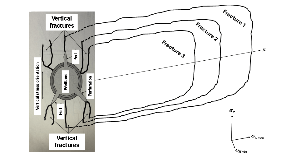
Fig. 1 is drawn to illustrate the initiation and propagation of multiple hydraulic fractures from a perforation cluster in a horizontal wellbore. It is expected that the vertical fractures are initiated from the perforation cluster if the vertical stress σV is the maximum stress, which is normally the case for vertical depths greater than 4000 ft. It is understood that the “fracture system” in the near wellbore area is complicated because the wellbore and perforations alter the state of the in-situ stresses in this area by a few times of the wellbore diameter. A number of fracture propagation phenomena could occur in this area. Fractures may reorient from the perforation towards the preferred fracture plane. Fractures may interact with and dilate fractures. The explosive energy during perforating could induce microcracks and initiate shear cracks. As a result, multiple and torturous fractures can be created in the near-wellbore area. Eventually, the fractures should propagate laterally in the direction of the maximum horizontal stress σHmax (fractures open against the minimum horizontal stress σHmin).

Figure 1: Illustration of spontaneous propagation of multiple fractures initiated from a perforation cluster.

When the fluid pressure at the tip of a perforation reaches the formation fracturing pressure, the formation breaks down, and the first fracture is initiated. The fluid pressure at the perforation tip will drop quickly to a level around the minimum horizontal stress σHmin. Keeping fluid injection at a constant flow rate will cause an increase in fluid pressure due to the flow friction inside the fracture as the fracture propagates. The propagation distance of the first fracture is expressed as:

x=(2n+22n+1C1)2n+12n+2t2n+12n+2(1)

where x in ft is fracture tip distance from the wellbore, n is the flow behavior index of fracturing fluid, t in seconds is fracturing fluid injection time, and the constant C1 is defined by:

C1=[372.25gqi(Pp−Pt)Khf]12n+1[0.5qi(3+1n)hf]n2n+1(2)

where g = 32.17 lbm-ft/lbf-s2 is gravitational acceleration constant, qi in ft3/s is fluid injection rate per half cluster (fractures propagate in both sides), Pp in lbf/ft2 is the pressure at the tip of perforation, Pt in lbf/ft2 is the pressure at fracture tip, K in cp is fluid consistency coefficient, and hf in ft is fracture height (assuming constant).

The dynamic average fracture width w in feet is expressed by

w=(2n+22n+1)qihf(2n+22n+1C1)2n+12n+2t12n+2(3)

When the fluid pressure at the tip of the perforation increases to the formation breakdown pressure again, the second fracture is initiated from the tip of another perforation. The width of the first fracture at the moment of the initiation of the second fracture is called the critical fracture width (wc). Xiao et al. [6] suggested that the following equation for the maximum fracture width at the wellbore is taken as the critical fracture width:

wm=3.28∗9.1512n+23.98n2n+2[1+2.14nn]n2n+2(0.001K)n2n+2[(0.3048hf)1−nxfQi11095E]12n+2(4)

where wm (ft) is the maximum fracture width under a constant flow rate of Qi = 2qi (ft3/s) for two fracture wings, K is the consistency index (cp), n is the fluid flow consistency index, E is the Young’s modulus of formation rock (lbf/ft2), xf is the half fracture length (ft), hf is the fracture height (ft). However, this maximum fracture width is fracture-length dependent. Without knowing the value of xf, the value of wm cannot be determined.

Use of the maximum fracture width at the wellbore as the critical fracture width is not rigorous. We propose a new approach to estimate the critical fracture width. It is understood that Eqs. (1) through (3) were derived from fluid hydraulics while Eq. (4) was derived based on rock elasticity. These two equations are independent. Assuming the critical fracture width is equal to the half of the maximum fracture width at the wellbore, combining Eqs. (1) through (3) and half of the value given by Eq. (4) should give a reasonable estimate of the critical fracture width. The derivation of method is as follows.

Solving for the injection time t from Eq. (3) gives

t=[whf(2n+22n+1C1)2n+12n+2qi(2n+22n+1)]2n+2(5)

Substituting Eq. (5) into Eq. (1)

x=(2n+22n+1C1)2n+12n+2[whf(2n+22n+1C1)2n+12n+2qi(2n+22n+1)]2n+1(6)

Substituting Eq. (6) into Eq. (4) for xf and renaming wm and w to wc = 0.5wm result in

wc=0.5(αβ)2n+2(7)

where

α=ab12n+2(8)

β=[hf(2n+22n+1C1)2n+12n+2qi(2n+22n+1)]2n+12n+2(9)

a=3.28∗9.1512n+2[0.00398K(1+2.14nn)]n2n+2(10)

and

b=qi(0.3048hf)1−n22,190E(2n+22n+1C1)2n+12n+2(11)

where the value of the critical fracture width wc is in ft.

Once the critical fracture width is determined, the critical time and critical fracture length for the first fracture can be predicted. According to Eq. (5), the time at which the second fracture is initiated is expressed by

tc=[wchf(2n+22n+1C1)2n+12n+2qi(2n+22n+1)]2n+2(12)

According to Eq. (1), when the second fracture is initiated, the tip of the first fracture is at

xc=(2n+22n+1C1)2n+12n+2tc2n+12n+2(13)

After initiation of the second fracture, assuming the first fracture will remain open with a width wc, the further growth of the first fracture is expressed as (see Xiao et al. (2019) for derivation):

x1=(xcn+1n+n+1nC1′t)nn+1−xc(14)

where t is the time starting from the initiation of the second fracture and

C1′=[372.25gw1(Pp−Pt)K]1n(0.5w13+1/n)(15)

where the average width of the first fracture (w1) after initiation of the second fracture is assumed to remain wc.

The fluid flow rate in the first fracture is diverted to the second fracture and is expressed by

q1=hfw1C1′(xcn+1n+n+1nC1′t)−1n+1(16)

The fluid flow rate in the second fracture is therefore expressed as

q2=qi−q1=qi−hfw1C1′(xcn+1n+n+1nC1′t)−1n+1(17)

The distance of the tip of the second fracture is expressed by

x2=(2n+22n+1C2)2n+12n+2t2n+12n+2(18)

where C2 is defined by

C2=[372.25gq2(Pp−Pt)Khf]12n+1[0.5qi(3+1n)hf]n2n+1(19)

Similarly, the initiations and propagations of sequential fractures can be formulated. A computer program FracPropag was developed in this study to speed up computations and plot sequential initiation and spontaneous propagations of multiple fractures created from a perforation cluster.

3  Model Validation

The result of the computer program FracPropag was compared with a real case to check accuracy. Fig. 2 provides recorded engineering parameters during a stage of hydraulic fracturing operation on a 130 ft-thick reservoir with a Young’s modulus of 8.82 Mpsi (60 Gpa). The peak value of the bottom hole pressure curve indicates that the formation breakdown pressure is about 14,000 psi, which is assumed to be the pressure at the perforation tip when the first fracture was initiated. The lowest value of the bottom hole pressure curve is about 12,700 psi, which is assumed to be the pressure at the fracture tip when the fracture was propagating. About 8800 bbl of water-based slurry (K = 1 cp and n = 1) was injected into 3 perforation clusters at an average pumping rate of 84 bpm. The bottom hole pressure curve in Fig. 2 suggests that 3 hydraulic fractures were created before proppant screen-out. The second fracture was initiated about 20 min after creation of the first fracture, i.e., the critical time for the first fracture is about 20 min. The third fracture was initiated about 60 min after creation of the second fracture, i.e., the critical time for the second fracture is about 60 min.

Figure 2: Engineering parameters recorded in a stage of hydraulic fracturing operation.

Table 1 shows the FracPropag-calculated hydraulic fracture generation and propagation data. It predicts that the critical time for the first fracture is 21.51 min and the critical time for the second fracture is 62.04 min. These values are remarkably close to those numbers identified from Fig. 2. It also suggests that the fourth fracture should have been created 111.04 min after initiation of the third fracture, should the proppant screen-out have not occurred. Fig. 3 demonstrates the creation of 3 hydraulic fractures computed by the program FracPropag.

Figure 3: Generation of hydraulic fractures predicted by the computer program FracPropag.

It is understood that the orientations of fractures presented in Fig. 3 is just for illustration purposes. They are not rigorously predicted because stress shadow effects are not considered in the model. Inclusion of the stress effect is much more complicated in multi-fracture systems and is beyond the objective of this study. Although the result of the mathematical model matches field data for this one case in the prediction of fracture generation, the mathematical model may not be accurate in other cases, especially for where natural fractures exist in the reservoir. Further studies are desirable in this research area.

It is also understood that the model assumes constant fracture height throughout the fracture propagation process. However, fracture height growth is commonly observed in shale formations. The assumption of constant fracture height should under-estimate the lateral propagation of fractures, especially in thick shale formations. Future research should address this issue for better modeling of fracture propagation.

It is further understood that natural fractures pose significant influence on the initiation and propagation trajectory of hydraulic fractures. Without having a good knowledge of locations of the natural fractures, which is normal, accurate prediction of hydraulic fracture propagation is impossible. The proposed model should be used with caution in naturally fractured shale formations.

It is very difficult to find clean datasets that would allow generation of error bounds on the predicted critical times and fracture length, which limits the practical utility of the model for engineering design. This issue should be addressed in future investigations.

4  Sensitivity Analysis for TMS

Tuscaloosa Marine Shale (TMS) is part of the Tuscaloosa Group deposited along the northern Gulf of Mexico during the Cenomanian to Turonian stages of the late Upper Cretaceous [18]. A total of 79 horizontal oil wells were drilled in the TMS between 2011 and 2015. Drilling activity in the TMS stopped in 2015 due to a downturn in oil prices. Resuming drilling activities is being considered using the new well-fracturing technologies developed in the past decade.

Pay zones of the TMS are the oil to condensate-wet gas zones with a Total Organics Content (TOC) ranging generally between 0.5% and 3% in 40% to 65% rich clay [19]. TMS porosity was measured by mercury porosimetry to be <4% with a permeability in a range between 10 to 79 nd, averaged 33 nd. However, based on the production data of 16 TMS wells in the Mississippi section of the TMS, the estimated permeability ranged from 53 to 210 nd, averaged 116 nd. The discrepancy between the lab-measured and production-data-derived permeabilities is attributed to natural fractures. Based on the studies conducted by Hackley et al. [20], the technically recoverable continuous resource of TMS has a mean value of 1537 million barrels of oil and 4614 billion cubic feet of gas.

The initial oil production rate of 79 TMS wells between 68 and 1266 bbl/d, averaged 586 bbl/d, of 85%–100% light crude oil (38°–45°API), with an initial GOR from 30 to 1050 scf/bbl, averaged 527 scf/bbl. The drop in well productivity was attributed to the fast decline rate of fracture conductivity between 0.20% and 0.74% per month [21].

For improving the productivity of future TMS wells, reducing perforation-cluster spacing and increasing the number of perforation clusters are the priorities. Increasing SRV is another means of improving well productivity. The following model analysis focuses on how to create more short fractures to increase fracture network complexity and thus SRV.

TMS has a total formation thickness ranging from 500 to over 800 feet. The specific “pay zone” or high-resistivity target zone, typically found at the base of this formation, is thinner, generally ranging from 0 to 325 feet (0 to 99 m) in thickness. TMS is characterized by high, abnormal formation pressures and requires high fracturing pressures for successful stimulation. It is overpressured in the range of 4366–9413 psi at depths of 10,000 to 15,000+ feet in Louisiana and Mississippi. Its pressure gradients typically range from 0.65 to 0.75 psi/ft. Drillers often increased mud weights to match pressures equivalent to 6200 psi to prevent blowouts when penetrating the TMS. Fracturing treatments in the TMS often require high injection pressures up to 15,000 psi. Its minimum horizontal stress, which directly dictates the pressure needed to create a fracture, increases with clay content, making some sections, especially those with high clay (over 50%), challenging to fracture. TMS often contains natural fractures, with increased frequency at depths of 10,940 to 11,055 feet. Based on analysis of the TMS and surrounding formations, the minimum horizontal stress varies due to the overpressured nature of the shale, but it is generally found to be high, with some studies indicating specific, localized values. A study on a specific, 20-foot-thick shale interval below the main TMS base identified an increase in minimum horizontal stress in that specific zone. Another specific, though not general, reference to a study at a demonstration site (Cranfield field) found the reservoir minimum total horizontal stress to be roughly 51 MPa (approximately 7400 psi), calculated for the Lower Tuscaloosa. Table 2 presents a data set for predicting the propagation of multiple hydraulic fractures in a generic TMS well where the pressure at the perforation tip is assumed to be the shale breakdown/fracturing pressure, and the pressure at the fracture tip is assumed to be the minimum horizontal stress.

Effect of Fluid Type on Fracture Divergence. Fluids are classified into distinct categories on the basis of their rheological behaviors. Fig. 4 shows five types of fluids that are often found in applications in industry. Curves characterize fluids that are most common in nature. The shear stress is directly proportional to shear rate, meaning that fluid viscosity, defined by shear stress divided by shear rate, is constant. Water and oil are examples of fluids in this category. These fluids are called Newtonian fluids. Curve b shows a linear relationship between the shear rate and shear stress except in the low-shear-rate region. The shear stress takes a non-zero value at zero shear rate. The viscosity of fluid drops with shear rate, called the shear-thinning effect. Fluids of this type are called Plastic fluids, or Bingham Plastic fluid. They can be obtained by adding clay-like solid particles to Newtonian fluids. Curve c shows a non-linear relationship between the shear rate and shear stress. They also have shear-thinning behavior. Fluids of this type are called pseudo-plastic fluids, or Power Law fluids. Polymer solutions, such as slick water, usually fall into this category. Curve d shows a non-linear relationship between the shear rate and shear stress with a non-zero shear stress value at zero shear rate. They also have shear-thinning behavior. Fluids of this type are called Herschel and Buckley fluids. Curve e also shows a non-linear relationship between the shear rate and shear stress. The apparent viscosity of fluid increases with shear rate, called the shear-thickening effect. Fluids of this type are called dilatant fluids, which can be obtained by adding starch-like materials (e.g., carboxymethyl cellulose or CMC) to Newtonian fluids.

Figure 4: Rheological behavior of distinct types of fluids.

The rheological behavior of fluids can be generally described by the Herschel and Buckley model as follows [22]:

τ=τy+Kγ˙n(20)

where τ is shear stress in lb/100 ft2 or Pa, τy is yield point in lb/100 ft2 or Pa, K is consistency index in cp or Pa-s, γ˙ is shear rate in s−1, and n is flow behavior index (dimensionless). Considering the fluids without yield point, when n < 1, the Herschel and Buckley model degenerates to a Power Law model, describing the shear-thinning behavior of pseudo plastic fluids. When n = 1, the Herschel and Buckley model describes the behavior of Newtonian fluids. When n > 1, the Herschel and Buckley model degenerates to a Power Law model, describing the shear-thickening behavior of dilatant fluids.

Fig. 5 presents FracPropag-calculated fracture propagation data during hydraulic fracturing with slick water (n = 0.9) at an injection rate of 30 or 10 bpm per perforation cluster. It predicts that two fractures are generated in 80 min when 2400 bbl of fluid is pumped. They should propagate to 7604 and 3815 ft, respectively. The critical pumping time for the first fracture is 29 min when the second fracture is initiated. The critical pumping time for the second fracture is 81 min when the third fracture is initiated.

Figure 5: Model-calculated propagation of hydraulic fractures for n = 0.9 and qi = 10 bpm.

Fig. 6 presents FracPropag-calculated fracture propagation data during hydraulic fracturing with water (n = 1.0) at an injection rate of 30 bpm. It predicts that three fractures are generated in 80 min. They should propagate to 4620, 4010, and 1919 ft, respectively. The critical pumping time for the first fracture is 11.09 min when the second fracture is initiated. The critical pumping time for the second fracture is 33.05 min when the third fracture is initiated. The critical pumping time for the third fracture is 60.04 min for the fourth fracture is initiated, if the pumping time is longer. Comparing the data in Fig. 6 to that in Fig. 5 implies that slick water should generate fewer fractures than water.

Figure 6: Model-calculated propagation of hydraulic fractures for n = 1 and qi = 10 bpm.

Fig. 7 presents FracPropag-calculated fracture propagation data during hydraulic fracturing with water (n = 1.1) at an injection rate of 30 bpm. It predicts that four fractures are generated in 80 min. They should propagate to 3184, 3029, 2615, and 1680 ft, respectively. The critical pumping time for the first fracture is 4.12 min when the second fracture is initiated. The critical pumping time for the second fracture is 13.56 min when the third fracture is initiated. The critical pumping time for the third fracture is 25.46 min when the fourth fracture is initiated. The critical pumping time for the fourth fracture is 38.70 min, when the fifth fracture would be initiated. Comparing the data in Fig. 7 to that in Fig. 6 implies that dilatant fluid should generate more fractures than water.

Figure 7: Model-calculated propagation of hydraulic fractures for n = 1.1 and qi = 10 bpm.

Comparison of data in Figs. 5 through 7 indicates that the number of short fractures should increase with the n-value of fracturing fluid. This is explained by the shear-thickening effect of fluid that should cause more friction in long and wide fractures, which will slow down fracture propagation.

Effect of Fluid Viscosity on Fracture Divergence. Fig. 8 compares FracPropag-calculated propagations of hydraulic fractures with n = 1.1, K = 10 cp and pumping rate qi = 10 bpm. A comparison of Figs. 7 and 8 shows that the number of fractures has increased, but the fracture lengths have reduced. This is because viscous fluid induce more friction in long fractures that will slow down fracture propagation.

Figure 8: Model-calculated propagation of hydraulic fractures generated by pumping fracturing fluid with n = 1.1, K = 10 cp and pumping rate qi = 10 bpm.

Effect of Fluid Pumping Rate on Fracture Divergence. Fig. 9 shows FracPropag-calculated propagations of hydraulic fractures for n = 1.1, K = 10 cp, and fluid pumping rates qi = 15 bpm after 2400 bbl of fracturing fluid is pumped. A comparison of Figs. 8 and 9 shows that the number of fractures has significantly increased, but the fracture lengths have reduced. This is because viscous fluid induces more friction in long fractures that will slow down fracture propagation.

Figure 9: Model-calculated propagation of hydraulic fractures n = 1.1, K = 10 cp and pumping rate qi = 15 bpm.

5  Conclusions

A previously presented analytical model for sequential initiation and simultaneous propagation of hydraulic fractures was modified in this study to include a technique for predicting the critical fracture width. The modification was made using a model to predict the maximum fracture width, accounting for rock elasticity. The modified model was coded in the FracPropag computer program. The program was validated using data from a real hydraulic fracturing operation. A sensitivity study was performed for the Tuscaloosa Marine Shale (TMS). The following conclusions are drawn.

1.    The new analytical model for sequential initiation and simultaneous propagation of hydraulic fractures takes a closed form with the critical fracture width determined implicitly. This makes it easy to implement the model in computer algorithms, thereby improving computational efficiency.

2.    The developed computer program, FracPropag, based on the analytical model, predicts the sequence of initiation of multiple hydraulic fractures that is consistent with that indicated by a bottom-hole pressure curve recorded in a real case of hydraulic fracturing operation. More case studies are desirable to validate the computer model’s reliability fully.

3.    The new analytical model predicts that, compared to water, the use of plastic fluids (e.g., slick water) should reduce the number of short hydraulic fractures and thus the fracture network’s complexity. This is attributed to the shear-thinning effect of the fluid, which reduces friction in long fractures. Compared with water, the use of dilatant fracturing fluids (e.g., CMC solutions) should increase the number of short hydraulic fractures and thus the complexity of the fracture network. This is attributed to the shear-thickening effect of the fluid, which increases the friction in fluid flow along long fractures.

4.    The new analytical model reveals that, regardless of fluid type, increasing fracturing fluid viscosity increases the number of short hydraulic fractures and thus the fracture network complexity. This is because fluid viscosity induces friction, hindering fluid flow in long fractures.

5.    The new analytical model suggests that, regardless of fluid type, using a high fracturing fluid pumping rate is always desirable to increase the number of short hydraulic fractures and thus fracture network complexity. This is because high fluid velocity induces greater friction, hindering fluid flow in long fractures.

Acknowledgement: The author is grateful to the administration of the Energy Institute of Louisiana of University of Louisiana at Lafayette for its administrative assistance throughout this research.

Funding Statement: This research was supported by the Louisiana Board of Regents Support Fund (BoRSF), Grant No. LEQSF(2024–27)-RD-B-04.

Availability of Data and Materials: The data supporting the findings of this study are included within the article.

Ethics Approval: Not applicable.

Conflicts of Interest: The author declares no conflicts of interest.

References

1. Weng X, Kresse O, Cohen C, Wu R, Gu H. Modeling of hydraulic fracture network propagation in a naturally fractured formation. In: Proceedings of the SPE Hydraulic Fracturing Technology Conference; 2011 Jan 24–26; The Woodlands, TX, USA. [Google Scholar]

2. Wu J, Liu Y, Yang H. New method of productivity equation for multibranch horizontal well in three-dimensional anisotropic oil reservoirs. J Energy Resour Technol. 2012;134(3):032801. doi:10.1115/1.4006573. [Google Scholar] [CrossRef]

3. Zhou D, Zheng P, Peng J, He P. Induced stress and interaction of fractures during hydraulic fracturing in shale formation. J Energy Resour Technol. 2015;137(6):062902. doi:10.1115/1.4030832. [Google Scholar] [CrossRef]

4. Manchanda R, Sharma MM. Impact of completion design on fracture complexity in horizontal wells. In: Proceedings of the SPE Annual Technical Conference and Exhibition; 2012 Oct 8–10; San Antonio, TX, USA. [Google Scholar]

5. Cheng Y. A mathematical model to predict fracture complexity development and fracture length [master’s thesis]. Lafayette, LA, USA: University of Louisiana at Lafayette; 2016. [Google Scholar]

6. Xiao D, Guo B, Zhang X. An analytical model for describing sequential initiation and simultaneous propagation of multiple fractures in hydraulic fracturing shale oil/gas formations. Energy Sci Eng. 2019;7(5):1514–26. doi:10.1002/ese3.421. [Google Scholar] [CrossRef]

7. Zhang N, Guo B. Use of mathematical model to predict the maximum permissible stage injection time for mitigating frac-driven interactions in hydraulic-fracturing shale gas/oil wells. J Energy Resour Technol. 2021;143(8):082901. doi:10.1115/1.4048870. [Google Scholar] [CrossRef]

8. Roussel NP, Sharma MM. Optimizing fracture spacing and sequencing in horizontal-well fracturing. SPE Prod Oper. 2011;26(2):173–84. doi:10.2118/127986-pa. [Google Scholar] [CrossRef]

9. Li S, Zhao H, Cheng T, Wang J, Gai J, Zou L, et al. The analysis of hydraulic fracture morphology and connectivity under the effect of well interference and natural fracture in shale reservoirs. Processes. 2023;11(9):2627. doi:10.3390/pr11092627. [Google Scholar] [CrossRef]

10. Liu X, Wang Y, Li T, Liang Z, Meng S, Zheng L, et al. Fractal-based modeling and quantitative analysis of hydraulic fracture complexity in digital cores. Mathematics. 2025;13(17):2700. doi:10.3390/math13172700. [Google Scholar] [CrossRef]

11. Yang K, Huang G, Zhou F, Liang T, Zuo J, Li M. Numerical simulation of hydraulic-natural fracture interaction based on the continuous–discontinuous element method. Sci Rep. 2026;16(1):4421. doi:10.1038/s41598-025-34508-z. [Google Scholar] [CrossRef]

12. Gong X, Jin Z, Ma X, Liu Y, Li G, Guo Y. Experimental study of the effect of natural fracture curvature on hydraulic fracture propagation behavior. Sci Rep. 2025;15(1):20716. doi:10.1038/s41598-025-07039-w. [Google Scholar] [PubMed] [CrossRef]

13. Shi X, Huang H, Zeng B, Guo T, Jiang S. Perforation cluster spacing optimization with hydraulic fracturing-reservoir simulation modeling in shale gas reservoir. Geomech Geophys Geo Energy Geo Resour. 2022;8(5):141. doi:10.1007/s40948-022-00448-5. [Google Scholar] [CrossRef]

14. Tian F, Jin Y, Shi L, Cong Z, Li Y. Simulation study on interactive propagation of hydraulic fractures and natural fractures in shale oil reservoir. Front Earth Sci. 2022;10:868095. doi:10.3389/feart.2022.868095. [Google Scholar] [CrossRef]

15. Yu H, Xu W, Li B, Huang H, Micheal M, Wang Q, et al. Hydraulic fracturing and enhanced recovery in shale reservoirs: theoretical analysis to engineering applications. Energy Fuels. 2023;37(14):9956–97. doi:10.1021/acs.energyfuels.3c01029. [Google Scholar] [CrossRef]

16. Li J, Zhong Y, Yan Y, Huang T, Mou Q, Yang B. Mechanism of hydraulic fracture propagation and the uneven propagation behavior of multiple clusters in shale oil reservoirs. Fuel. 2025;395:135241. doi:10.1016/j.fuel.2025.135241. [Google Scholar] [CrossRef]

17. Yang L, Wang X, Niu T. Propagation characteristics of multi-cluster hydraulic fracturing in shale reservoirs with natural fractures. Appl Sci. 2025;15(8):4418. doi:10.3390/app15084418. [Google Scholar] [CrossRef]

18. Lu J, Milliken K, Reed RM, Hovorka S. Diagenesis and sealing capacity of the middle Tuscaloosa mudstone at the Cranfield carbon dioxide injection site. Environ Geosci. 2011;18(1):35–53. doi:10.1306/eg.09091010015. [Google Scholar] [CrossRef]

19. Lu J, Ruppel SC, Rowe HD. Organic matter pores and oil generation in the Tuscaloosa marine shale. Bulletin. 2015;99(2):333–57. doi:10.1306/08201414055. [Google Scholar] [CrossRef]

20. Hackley PC, Enomoto CB, Valentine BJ, Rouse WA, Lohr CD, Dulong FT, et al. Assessment of undiscovered continuous oil and gas resources in the Upper Cretaceous TMS of the U.S. Gulf Coast, 2018. Reston, VA, USA: U.S. Geological Survey; 2018. [Google Scholar]

21. Mokhtari M, Mariana Ruse C, Yang X, Wortman PB, Guo B. Clay-rich tuscaloosa marine shale: production decline analysis. In: Proceedings of the Unconventional Resources Technology Conference; 2024 Jun 17–19; Houston, TX, USA. [Google Scholar]

22. Liu G. Applied well cementing engineering. Houston, TX, USA: Gulf Professional Publishing; 2021. p. 254–5. [Google Scholar]