
 Submit a Paper
 Propose a Special lssue
 Open Access
ARTICLE

Intelligent Operation Strategies for PVT-ASHP Heating and Hot Water Systems in Industrial Parks Based on Reinforcement Learning
1 Building Energy and Environment Research Institute, Sichuan Institute of Building Research, Chengdu, 610084, China
2 School of Thermal Engineering, Shandong Jianzhu University, Jinan, 250101, China
3 School of Mechanical Engineering, Southwest Jiaotong University, Chengdu, 610030, China
* Corresponding Authors: Jiying Liu. Email: ; Bo Gao. Email:
Energy Engineering 2026, 123(7), 2 https://doi.org/10.32604/ee.2025.074454
Received 11 October 2025; Accepted 17 December 2025; Issue published 18 June 2026
 View Full Text
 Download PDF
Abstract
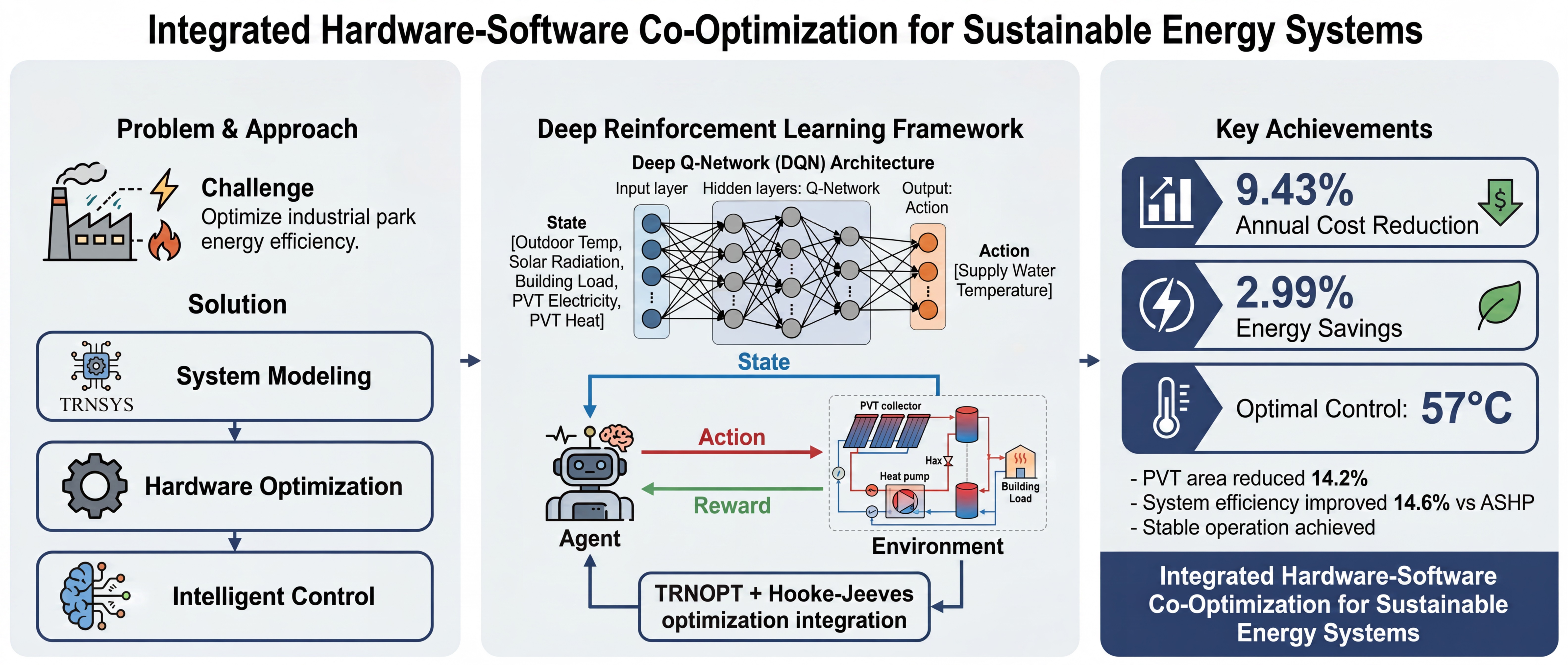
In response to the high energy consumption, large load fluctuations, and insufficient adaptability associated with conventional control strategies in industrial park heating and hot water systems, this paper studies a 15,000 m2 factory office building in Jinan as its object of study. A photovoltaic-thermal integrated air-source heat pump system (PVT-ASHP) is developed. This system leverages its hardware parameter co-optimization and intelligent operational strategy control to perform cost reduction and efficiency increase, while focusing on the novel innovative high effectiveness of its operational strategies. The study first employs the Hooke-Jeeves algorithm to optimize key hardware parameters so as to minimize the annual cost, perform many adjustments, including the reduction of the PVT collector area from 931 to 799 m2, regulate the PVT tilt angle from 36° to 43°, and modify the storage tank volume. This allows for the establishment of a low-energy baseline, reducing the initial PVT equipment investment by approximately 14.2%. In addition, the PVT photovoltaic efficiency is stabilized at 14%, while the solar thermal efficiency fluctuates around 33%. The core operational strategy uses a reinforcement learning algorithm based on Deep Q-Network (DQN). Its design incorporates dual variables PVT electricity generation (PVTd) and PVT heat supply (PVTh) into the state space, which overcomes the limitations of conventional control relying solely on load and outdoor temperature to perform dynamic matching between energy production and load demand. The reward function comprises dynamic weighting for energy consumption and comfort, where the energy consumption weight and comfort weight are set to 0.9 and 0.1, respectively. Based on the office hours of the factory (8:00–18:00 as high load, and non-office hours as low load), an hourly load input mechanism is designed to remove the control deviations caused by the average load assumption. Simulations are then conducted. The obtained results demonstrate that, compared with the conventional control strategy of fixed temperature at 60°C, the designed DQN reinforcement learning operation strategy achieves energy savings of about 2.99%. During office hours, the system maintains a stable supply water temperature of 57°C, which is consistent with comfort requirements while avoiding energy waste. After performing parameter optimization using the operational control strategy, the annual operating costs of the system decrease by 9.43%, while significantly increasing the overall energy efficiency. This paper demonstrates that the proposed DQN reinforcement learning operation strategy, tailored to the load characteristics of factory campuses, plays an important role in improving system performance. Based on the principles of dynamic perception, precise matching, and demand-driven regulation, it provides a potential reference framework for designing similar systems to ensure the efficient operation of distributed energy systems in factory campus-type buildings.Graphic Abstract
Keywords
The building sector plays a crucial role in the global energy consumption landscape, accounting for 20%–40% of the total energy use [1]. Advanced control strategies demonstrate high potential in increasing energy efficiency, reducing operational costs, and ensuring occupant comfort through precise and adaptive building system regulation capabilities [2]. Therefore, it is essential to optimize the operation of air-source heat pump units to reduce building energy consumption, serving as one of the pathways to achieving carbon peaking and carbon neutrality in buildings [3].
The construction industry accounts for a large portion of global energy consumption [4]. Solar heating, a clean alternative, can significantly reduce the dependence on fossil fuels, contributing to the achievement of emission reduction targets [5]. It has been widely applied due to its low-carbon and environmentally friendly characteristics [6]. Air-source heat pump systems have become a key approach in building heating due to their flexible installation and wide application range [7]. Photovoltaic-thermal (PVT) and air-source heat pump (ASHP) coupled water heating systems, referred to as PVT-ASHP in this paper, provide unique advantages in distributed energy utilization by simultaneously generating electricity and providing heating. Their synergistic operation significantly reduces the dependence on conventional energy sources [8].
In the context of PVT heating systems, Lee et al. [9] argued that existing studies mainly focused on short-term performance, with insufficient experimental validation and limited economic assessment. To address these limitations, they developed and validated a TRNSYS18-based simulation model for analyzing the long-term operational performance and economic feasibility of such systems subjected to high thermal loads. Their results demonstrated that the system leverages PVT seasonal heat to increase the heating performance and energy efficiency, while reducing fluctuations in the heat pump coefficient of performance (COP) and maintaining stable power consumption. Kamel and Fung [10] proposed an integrated system combining building-integrated PVT and ASHP, enabling an increase in the overall COP and the energy efficiency of the building. Brahim Taoufik [11] studied the long-term operation performance of PVT coupled heat pump systems by analyzing the feasibility of a dual tank indirect parallel solar-assisted heat pump system. They then verified its energy and economic advantages throughout the lifecycle. Chaouch et al. [12] proposed an energetic and exegetic analysis method of a long-term nonlinear dynamic rolling PVT collector model under typical Tunisian (North Africa) climate conditions. Their results provided a theoretical basis for the evaluation of the performance of PVT systems under various operational scenarios. Yu et al. [13] employed the Hooke-Jeeves algorithm to optimize key parameters of the PVT heating system, thereby reducing its annual cost. However, their study lacked an optimized system control strategy; Wang et al. [14] developed a TRNSYS-based simulation model for coupled phase change tank PVT-ASHP hot water systems addressing key parameter design issues. Using a residential building in Zhengzhou as the case study, they analyzed the impact of four critical parameters (i.e., hot water storage tank volume, PVT area, tilt angle, and circulation flow rate) on the system performance. They aimed at increasing the overall efficiency by conducting orthogonal experiments and range analysis to determine the impact level of these parameters and identify their optimal values. Their results demonstrated that the descending order of their impact is given by: tank volume, PVT area, circulation flow rate, and tilt angle. After identifying the optimal values, the overall efficiency reached 76.28%. These results provided a theoretical basis for the optimization of the performance design of PVT-ASHP hot water systems.
Many studies have been conducted on the development of integrated hot water systems that combine renewable energy with high-efficiency heat pump technology, performing their dynamic optimization through intelligent control strategies [15]. Reinforcement learning (RL) has made significant progress in its application to building energy systems [16], such as HVAC optimization. For instance, Yu et al. [17] used deep RL (DRL) along with model predictive control to perform significant energy reduction while maintaining thermal comfort in multi-zone buildings. Gu et al. [18] proposed an automatic optimization method for parallel energy consumption prediction based on RL, allowing for automatic optimization of model hyperparameters for accurately forecasting air conditioning energy consumption. They then conducted many experiments on real air conditioning datasets provided by five factories, demonstrating that their method outperforms existing prediction solutions, achieving average accuracy and performance increases of 11.48% and 32.48%, respectively. Li et al. [19] studied demand response control for air conditioning systems, noting that conventional approaches for determining thermostat settings rely on predefined models. They employed a near-term policy optimization RL algorithm, using a neural network to establish a policy framework for determining discrete control actions. They adopted a novel objective function truncation method to constrain the update steps, so as to increase the robustness of the algorithm. Their results demonstrated that this algorithm performs temperature setpoint control, yielding a 9.17% reduction in operating costs compared with non-heat-storage air conditioning systems exhibiting constant setpoints. Xia et al. [20] proposed an adaptive optimization scheduling strategy for residential HVAC based on DRL. This approach considers the scheduling problem as a Markov decision process. It adaptively learns state transition probabilities to make cost-effective decisions under tolerance violations. Their results demonstrated that the adaptation of the residential HVAC scheduling strategy to real-time electricity price signals from demand response programs and ambient temperature allows for a significant reduction in the electricity costs while maintaining occupant comfort; Zhang et al. [21] applied RL to supply-side control of HVAC systems. They adopted Q-learning and Deep Q-Network (DQN) as case studies, and dynamically controlled the number of pumps, their frequency, and supply water temperature based on outdoor dry-bulb temperature and building cooling load. Their pre-training results showed energy savings of 4.70%/4.65% and −0.66%/1.28% for DQN and Q-learning training/testing data, respectively. DQN and Q-learning significantly outperformed historical control strategies. Their overall savings respectively reached 9.28% and 9.04% compared with rule-based control. This demonstrated the high ability of their framework to support real-world learning of RL agents.
The aforementioned studies provide important theoretical references for the application of RL to the proposed PVT-ASHP system. Existing research explored multi-energy flow coordination. However, few studies have focused on the integration of hardware parameters within industrial park scenarios [22]. Applications of RL have been limited to residential or small-scale building scenarios, while studies addressing hot water systems in commercial buildings (e.g., office towers within industrial parks) are insufficient [23]. In addition, existing control strategies fail to fully leverage the dual electrical and thermal output characteristics of PVT components. John and Kaltschmitt [24] developed a simulation model and a controller using RL methods to achieve cost-effective flow control. Their results demonstrated that the successfully trained control unit based on RL can reduce the operational costs using an independent validation dataset.
To solve the aforementioned problems, this paper studies the PVT-ASHP coupled hot water system in an industrial park office building. It employs the Hooke-Jeeves optimization algorithm to perform systematic collaborative optimization of the main operational parameters of the system. Based on the economically optimal configuration, it studies optimized operational strategies by developing an RL-based intelligent control approach for dynamic system optimization. In the state-awareness dimension, this study incorporates many parameters (e.g., building hot water demand, solar irradiance, outdoor temperature, PVT power generation, and heat collection) into the system state space to capture environmental and system dynamics. For control algorithm implementation, it uses the DQN algorithm instead of the conventional Q-Learning. In addition, it uses deep neural networks (DNNs) to model complex state-action mapping relationships, which significantly increases the processing capability for high-dimensional variables. The optimization objectives of this study consist of reducing the total energy consumption and minimizing the operating costs while ensuring user satisfaction with hot water supply, so as to perform synergistic optimization.
The results obtained in this study provide a robust theoretical support for the intelligent management of distributed energy systems in industrial parks, driving the development of renewable energy hot water systems toward high efficiency and low operating costs. By incorporating artificial intelligence, particularly RL, it proposes an autonomous learning and decision-making strategy that maximizes the energy-saving and cost-reduction of PVT-ASHP systems.
This paper tackles the development of digital models of office buildings using the SketchUp 3D modeling technology, while extracting thermal load parameters and considering them as simulation inputs. A PVT-ASHP heating system simulation model is developed using the TRNSYS dynamic simulation platform. The GENOPT module in TRNSYS is employed to apply the Hooke-Jeeves algorithm for equipment optimization. In addition, a DRL algorithm, which uses DQN to construct an agent, is introduced. The agent autonomously learns through continuous interaction with the heating system simulation environment, allowing it to dynamically optimize the control strategy for the heating system of the underlying building. The technical roadmap of this study is illustrated in Fig. 1.

Figure 1: Technical roadmap of this study
The concept of the PVT system was first proposed in 1978 [25]. Fig. 2 presents a PVT-ASHP-based heating system. During operation, the heat pump system produces hot water and transfers it to a thermal storage tank, also serving as a buffer tank. This reduces the number of starts and stops for the air-source heat pump, thereby extending the equipment’s lifespan. When heating demand increases, the thermal storage tank supplies the required hot water to users. The return water from users passes through the PVT system, where it is reheated, increasing the temperature of the thermal storage tank.

Figure 2: Schematic diagram of the PVT-ASHP system
In the development of the PVT-ASHP model, this paper adopts a parameter design methodology from solar-assisted heat pump systems to enhance the model’s adaptability for long-term operation and special climatic conditions [14]. Its core components comprise thermal storage tank modules, user, PVT, grid-connection, and energy storage modules. By generating green electricity for the system, the PVT component reduces the system’s energy consumption required by air-source heat pump systems, thereby further optimizing the energy management.
(1) Air-source heat pump model
The heating capacity (Qh) of the heat pump unit is expressed as [26]:
where qm,r is the refrigerant mass flow rate, hcr,in and hcr,out are the inlet and outlet refrigerant specific enthalpy, respectively.
qm,r is calculated as:
where ηv, Vh and vsuc are the volumetric efficiency, discharge volume, and suction specific volume of the compressor, respectively.
(2) PVT power generation model
The output power of photovoltaic power generation is the amount of electrical power that a photovoltaic system converts from solar energy and delivers to the grid or load within a given time period. The output power of the photovoltaic cell (Epv) is calculated as [27]:
where Epv, Sstc, and tstc are respectively the output power of the photovoltaic cell, solar irradiance, and ambient temperature under standard conditions, S and t are respectively the solar irradiance and ambient temperature under actual conditions, and
(3) PVT collector model
The steady-state heat transfer model for the collector is developed based on its energy balance with the concentrator. This can be expressed as [27]:
where Qloss is the heat loss of the heat pipe, Qenv and Qabs are respectively the solar radiation heat absorbed by the casing and the heat-absorbing pipe, Qao_gi, rad and Qgo_a,conv are respectively the radiative and convective heat transfer between the outer surface of the casing and the environment, Qgi_go,cond and Qao_ai,cond are respectively the conductive heat transfer between the inner and outer surfaces of the casing and the absorber tube and the heat transfer fluid.
When neglecting the heat loss in the pipes, the heat output QPTC of the collector system (QPTC) becomes equal to
(4) Storage tank model
Under ideal conditions (i.e., the temperature is uniformly distributed throughout the thermal storage tank and heat losses in the storage system are negligible), the energy available in the thermal storage system, represented by its instantaneous heat output (
where M is the mass of the thermal storage fluid, cp,oil is the specific heat capacity at constant pressure of the thermal storage medium, Toil,hot and Toil,cold are the temperatures of the hot and cold thermal storage fluids, respectively.
(5) Energy storage battery model
The specific mathematical expressions for energy storage batteries are given by Eqs. (11) to (15) [29]:
where
In addition, the state of charge and remaining capacity of the battery should be constrained, as follows:
where Et is the remaining battery charge at time t, ηc and ηd are respectively the charging and discharging efficiencies of the battery, SOCmin and SOCmax are respectively the lower and upper limits of the remaining battery charge.
2.2 Case Design Based on Jinan Region
Jinan City is located in the cold region of the building thermal design zone. Meteorological data for Jinan City are generated by the Meteonorm meteorological data software, which uses the 1991–2010 meteorological data as its default standard. Figs. 3 and 4 show the hourly temperature and solar radiation variations for Jinan City, respectively. According to the Technical Standard for Application of Solar Water Heating Systems in Civil Buildings (GB 50364-2018), the annual average total solar radiation at horizontal surfaces in Jinan is equal to 5125.72 [MJ/m2·a], and thus it is classified as a Region III area with abundant solar resources. In this region, the guaranteed solar energy utilization rate is in the range of 40%–50%.

Figure 3: Hourly temperature variation in Jinan City

Figure 4: Hourly solar radiation variation in Jinan City
An office-type building in a Jinan factory park is selected for this study. It has a floor area of 15,000 m2, 10 above-ground floors, and no basement. The per-capita office area is 4 m2, and the maximum daily per-capita water consumption is 8 L. The daily office hours and heating season are 8 a.m.–6 p.m., and 15 November–15 March of the next year, respectively. The maximum design heat load, hourly heat supply ratio, and daily facility hot water use time are equal to 1335, 156.31, and 10 h, respectively. Fig. 5 shows the building design heat load diagram. The hour-by-hour water use ratio is presented in Table 1.

Figure 5: Building design heat load diagram

Properly matched equipment has become crucial for reducing operational costs and increasing operational efficiency. The total area of solar collectors can be calculated as:
where AC is the total collector area of the direct system, QW is the average daily hot water consumption, CW is the specific heat capacity of water at constant pressure, ρw is the density of water, tend and t0 are the final design temperature of hot water and initial design temperature of cold water in the storage tank, respectively, JT is the annual average daily solar radiation on the collector surface at the local site, f is the solar energy availability factor for the solar water heating system in different solar resource zones, ηcd is the annual average collector efficiency based on total area, ηL is the heat loss rate in the storage tank and piping of the solar collector system (empirically set in the range of 0.20–0.30), qr is the average daily hot water consumption quota, m is the number of users, and b1 is the same-day usage rate.
In centralized solar water heating systems with collective heat collection and distribution, the storage tank and the hot water supply tanks should be installed in series. The effective volume of the hot water storage tank (Vrx) is calculated as:
where Aj is the total collector area, qrjd is the volume of hot water produced per unit area of collector with an average daily temperature increase of 30°C. For direct systems in regions with abundant Class III resources, qrjd is in the range of 50–60 L/(m2·d).
The volume utilization coefficient (r) is given by:
where Ad is the photovoltaic cell area and Aj is the total collector area.
Table 2 presents the selection of key equipment parameters for the system based on Eq. (21) along with engineering experience.

2.3 Establishment of a TRNSYS-Based Simulation Platform
The PVT-ASHP system is developed using the TRNSYS dynamic simulation platform. The flowchart of its operation is shown in Fig. 6. When users require heating or hot water, the thermal storage tank fulfills the water supply function. If the tank water temperature reaches 60°C (or higher), it directly meets supply standards, eliminating the need for the air-source heat pump to activate supplementary heating. Hot water can then be directly delivered to the users. When the tank temperature falls below the required 60°C, the air-source heat pump activates to raise the water temperature.

Figure 6: Flowchart of the PVT-ASHP system operation
When the PVT heating module is within the preset time period, it is automatically activated, maintaining continuous operation for both heat collection and electricity generation. The thermal energy it captures from solar radiation is used to increase the temperature of the thermal storage tank. The generated electricity, processed by the inverter, is prioritized for the own consumption of the system. When the electricity generation of the PVT module is greater than the power consumption of the system, the surplus electricity is first stored in the battery. If it is also greater than the storage capacity of the battery, the remaining portion is provided to the municipal grid. On the contrary, when the output of the PVT module is insufficient to meet the electricity demand of the system, stored energy from the battery is first used. If the battery cannot fully cover the shortfall, supplementary power is drawn from the municipal grid.
This study develops single ASHP and PVT-ASHP models with consistent key equipment parameter settings. The main components of ASHP include the air-source heat pump, water pump, thermal storage tank, and terminal units, while those of PVT-ASHP include the air-source heat pump, PVT, thermal storage tank, battery, and terminal units. Figs. 7 and 8 show the diagrams of the PVT-ASHP and ASHP models, respectively.

Figure 7: Diagram of the PVT-ASHP model

Figure 8: Diagram of the ASHP model
To validate the reliability of the PVT model, it is compared with the measured data provided in [30]. In the latter study, the city of Vicenza in the Veneto region, featuring a PVT area of 24 panels × 1.65 m2, is taken into consideration. Local meteorological parameters are imported using the Meteonorm software to develop a similar model. The results of the comparison are shown in Table 3. It can be seen that the simulated data are consistent with the experimental ones. The relative errors for the average daily heat output and electricity generation of the PVT collector are equal to 2.94% and 3.49%, respectively. These errors fall within an acceptable range, demonstrating that the proposed numerical model has high reliability.

2.4 Hooke-Jeeves Optimization Algorithm
The Hooke-Jeeves algorithm is commonly used for solving optimization problems [31]. In this algorithm, the distance between the last and the current solutions is recorded. If it is null, it is considered as one of the indicators for the termination condition. Otherwise, the current step size is multiplied by a number in the range of 0–1 such that
where ΔK is the step size, Δ0 is its initial value, and γK is a v factor in the range of 0–1.
Eq. (23) can be rewritten as:
Let
and thus:
It can be seen from Eq. (26) that, when K approaches infinity, the product becomes null. After developing the system operation model in TRNSYS and setting the objective function as minimizing operating costs, the Hooke-Jeeves algorithm in the GENOPT module is selected. Many parameters (e.g., step size and maximum number of iterations) are configured, the adjustable optimization variables and their ranges are defined, and a connection between the two is established through the GENOPT interface. Upon initiating optimization, GENOPT continuously adjusts variable values according to algorithmic rules, then provides parameter combinations to TRNSYS for simulation. TRNSYS calculates the objective function value and returns it until convergence criteria are met. Finally, the optimal parameter combination and objective function value output by GENOPT are analyzed, and their feasibility within TRNSYS is validated. The operational workflow of TRNSYS calling GENOPT is illustrated in Fig. 9.

Figure 9: Flowchart of TRNSYS calling GENOPT
2.5 Reinforcement Learning Deep Q-Network (RL DQN)
DQN is a representative DRL method, providing significant improvements over conventional Q-learning [33]. It approximates Q-values by leveraging the high capability of DNNs to extract complex features as well as their very high generalization ability. This design provides crucial support for adapting to complex scenarios. During training, DQN incorporates a replay buffer to effectively break data correlations, thereby avoiding model convergence issues caused by highly correlated training samples. It avoids direct updates to the Q-value of the current state by computing target Q-values through an objective network, which significantly increases the training stability [34]. Due to these characteristics, DQN has been widely applied to various domains, including gaming [35], robotics control [36], and transportation [37].
The main concept of DQN is to train a Q-network that takes the current state of the environment as input and outputs the Q-values for all actions available to the agent. The latter selects the action exhibiting the highest Q-value as its current action, and repeats this process until the round ends [38]. The operation of RL DQN is illustrated in Fig. 10.

Figure 10: Operation of RL DQN
In the agent’s exploration process, it selects an action as based on the current environment state Ss. The environment then assigns a reward value rs based on the quality of as. Afterwards, the environment transitions to the next state ss+1. Ss, as, rs, and ss+1 are then stored as a tuple in a list. This list, filled with (Ss, as, rs, ss+1), is used in the sequel to update the Q-network. This approach exemplifies the concept of experience replay, where the list plays the role of the experience replay buffer. The specific update employs temporal difference learning principles. The Q-learning update is expressed as [39]:
where Q(ts, as) is the Q-value for selecting action as in state ts. α is the learning rate, which controls the magnitude of Q-value updates, rs is the reward obtained at time step s, γ is the discount factor, used to measure the importance of future rewards, and
In the DQN algorithm, the update principle mirrors that of Q-learning. The Q-network is used to compute the values on the two sides of the formula, and the parameters of the network are then updated to make the value on the left-hand side approach that on the right side as much as possible.
2.6.1 Development of a Markov Decision Process
RL refers to an agent learning through continuous interaction with a complex, uncertain environment to maximize the obtainable rewards [40]. This is typically modeled as a Markov decision process comprising five core elements: a finite set of states (S), the action space of the agent (A), transition probabilities between states (P), rewards (R), and the discount factor (γ). A description of the Markov decision process is shown in Fig. 11.

Figure 11: Markov decision process description
State Variables: They are composed of four system operating parameters: the current system heat load (CLh), outdoor wet-bulb temperature (Tout), solar radiation intensity (SR), PVT electricity generation (PVTd), and PVT heat supply (PVTh). CLh serves as the core thermal demand that PVT-ASHP systems should meet in real time. It determines the degree of load matching and adjustment direction for system operation. It is the fundamental basis for state variable requirements. Tout reflects the comprehensive outdoor environmental temperature and humidity conditions. It significantly affects the heat exchange efficiency of the ASHP and the heat dissipation effectiveness of the PVT. It is a key external environmental parameter affecting the system. SR serves as the core energy source for the electricity generation and heating functions of the components of the PVT, correlated with its energy output potential. It is the fundamental parameter characterizing the energy input state of the PVT. PVTd reflects the power generation performance state of the PVT module. It is directly calculated by the monitoring system, and thus it is more precise than derived values, accurately reflecting the electrical output level of the PVT. PVTh characterizes the heating contribution state of the PVT module. It is also directly calculated by the monitoring system, it has higher precision than derived results and serves as the key energy output feedback for the heating side of the system.
Control Action: The heating water temperature of the air-source heat pump unit serves as the decision variable for RL, exhibiting a control step size of 1°C. The temperature setting range is based on the design temperature for facility hot water of approximately 60°C. This accounts for the impact of severe winter conditions on air-source heat pumps in cold regions while ensuring that the supply temperature remains within the acceptable range for the air-source heat pump, (i.e., 56°C–65°C) [41].
Reward Function: The core optimization objective consists in maximizing the energy efficiency while ensuring indoor thermal comfort, as the heating water temperature affects the energy consumption of air-source heat pumps and the heating performance at the terminal units. In the case of very low temperatures comfort requirements cannot be met, while in the case of very high temperatures energy efficiency requirements cannot be met. However, users can adjust water temperature at the terminal to ensure comfort. Based on this principle, a reward function, which integrates comprehensive energy consumption, comfort metrics,
and renewable energy utilization, is established while taking renewable energy application into consideration. It is given by [42];
where K1 and K2 respectively represent the weights between energy consumption and comfort level such that K1 + K2 = 1, Popt and Pref respectively denote the optimized and rated energy consumption of the air-source heat pump unit, Tre,gong is the heating hot water temperature, and Tre represents its upper limit value. The difference between the latter values reflects whether the provided heating capacity is sufficient. ∂1 and ∂2 are coefficients determined through regression analysis. Note that, in the conducted case study, K1 = 0.9, K2 = 0.1, ∂1 = 0.5, ∂2 = 0.14, and Tre = 55°C.
2.6.2 Hyperparameter Tuning of the DQN
In the implementation of the DQN, the agent employs an ε-greedy policy to balance exploration and exploitation. ε is initially set to 1, then linearly decreases at a rate of 0.0005 per step, reaching a minimum value of 0.01. This ensures thorough exploration in the early training phase and gradual convergence toward the optimal policy in later stages. The neural network architecture employs a dual-network structure comprising a policy network and an objective network. These two networks consist of two hidden layers (each containing 24 neurons) and an output layer of 10 neurons. The hidden layers use the ReLU activation function, while the output layer employs a linear activation function to estimate the Q-values. The network parameters are initialized through random uniform distribution. In the optimization process, γ, the batch size (Batch_Size), α, the number of training iterations, and the experience replay buffer capacity are set to 0.99, 128,1 × 10⁻⁴, 300, and 1 × 10⁶, respectively. This configuration significantly increases the learning stability and convergence speed of the algorithm through a stable target network update mechanism and data sampling strategy. The parameter settings are as shown in Table 4. The implementation is conducted on a workstation equipped with an AMD Ryzen 9 5950X 16-Core Processor (3.40 GHz), a Radeon graphics card (RX 550/550 series), 64 GB of RAM, and Windows 11, with a total training duration of 60 h.

2.6.3 Comparative Strategy Plan
Table 5 presents a comparison between four schemes. These schemes are detailed as follows:

Scheme 1: This approach combines the prediction capabilities of the TRNSYS model with an RL framework. The TRNSYS model uses historical data to forecast future trends in thermal load, integrating the utilization of renewable energy from the PVT system. When making decisions, the agent considers the CLh of the current state while incorporating Tout, SR, PVTd, PVTh, and the state composition (S = [CLh, Tout, SR, PVTd, PVTh]). When selecting control actions, it iterates through all the possible setpoints for the heating hot water supply temperature in the range of 56°C–65°C so as to optimize the control strategy.
Scheme 2: This method only controls the impact of PVT system power generation on the system. The agent selects control actions based solely on current environmental factors (S = [CLh, Tout, SR, PVTd]), where the state comprises the current cooling load, outdoor temperature, solar radiation, and PVT power generation. This aims at comparing and validating the impact of the solar thermal information on the optimization effectiveness.
Scheme 3: This method controls only the impact of the PVT system heating output on the system. The agent also selects control actions based solely on S = [CLh, Tout, SR, PVTh], where the state comprises current cooling load, outdoor temperature, solar radiation, and PVT heating output. This aims at comparing and validating the impact of the photovoltaic information on the optimization effectiveness.
Scheme 4: This method adopts fixed-temperature control, which is a control strategy adopted in conventional systems. Based on the design facility hot water supply temperature, the supply temperature of the unit is set to 60°C. In specific application scenarios, for existing PVT-ASHP systems, the impact of the PVT on the system is temporarily neglected.
2.7 Operational Evaluation Model
2.7.1 Coefficient of Performance for Heating (COPh)
The COPh of an air-source heat pump is the ratio of the heating (or cooling) capacity of its system to the consumed electrical power [43]:
where Qh is the heating capacity of the unit, Pc and Pb are respectively the compressor and fan power, and κ is the frosting and defrosting efficiency loss (equal to 0.95) [44].
2.7.2 Heat Pump Energy Consumption
The power of the heat pump unit is determined using an energy consumption model provided by the American Society of Heating, Refrigerating and Air-Conditioning Engineers (ASHRAE), It is computed as:
where Q is the cooling capacity, Tci is the inlet air temperature of the air-source heat pump unit, TWO is the outlet temperature of the user-side unit, and a, b, c, d, e, and f are unknown parameters.
Note that a-f, determined using the nonlinear least squares algorithm, are equal to −2.668739, −2.123145, 5.288032, 26.811261, −0.874554, and −30.748398, respectively.
The PVT instantaneous photoelectric efficiency (ηd) affects the real-time performance of solar energy conversion into electricity [45]. It is computed as:
where Epv is the output power of the photovoltaic cell, Ad is the area of the photovoltaic panel, and Iz is the total irradiance on the illuminated surface.
2.7.4 Solar Thermal Efficiency
The solar thermal efficiency of PVT solar collectors (ηr) reflects their ability to convert solar energy into thermal energy. It is computed as:
where: qw is the circulating water flow rate of the PVT solar collector, cp is the specific heat capacity of water at constant pressure, Tout and Tin are respectively the outlet and inlet water temperature of the collector, and Aj is the area of the PVT collector plate.
3.1 Optimization of the Annual System Operation Cost
3.1.1 Analysis Based on the Dynamic Calculation of Annual Value Method
To determine the annualized cost value, the dynamic calculation method allocates the initial investment across each year of the full lifecycle of the system based on the capital recovery formula, then adds this amount to the operating costs for this year. This method converts all the costs into a common present value standard and comprises all the factors affecting the economics of the system throughout its entire lifespan [46]. An improved dynamic annualized cost calculation method is employed to account for the reduced power generation from photovoltaic panels. This method calculates the annual cost (Z) as:
where is is the deposit interest rate (3% in Shandong Province), ny is the system lifespan (set to 20 years), L0 is the initial system investment, C is the equipment depreciation cost, R is the renewable energy compensation cost with electricity purchase and sale set to 0.6 and 0.4 Yuan, respectively.
The initial investment costs of the equipment, primarily sourced from China in 2022, are shown in Table 6.

3.1.2 Implementation of the Hooke-Jeeves Algorithm Using the GENOPT Module
In PVT solar thermal systems, the intensity of solar radiation is the key factor affecting the heat collection efficiency. It is highly correlated with the collector area, azimuth angle, and tilt angle. The size of the thermal storage tank affects both the heat collection efficiency and heat pump performance of the system, while the heat pump capacity also significantly affects the collector system [28]. The battery capacity determines the electricity storage capability of the photovoltaic power generation system. When optimizing PVT heating systems using the dynamic cost-per-year method, many optimization variables are selected, including the PVT collector area, tilt angle, azimuth angle, tank volume, heat pump heating capacity, and battery capacity.
The Hooke-Jeeves algorithm comprises a penalty mechanism for the optimization of the objective function within defined penalty constraints. It assigns monetary penalties corresponding to the objective function units, ensuring stable and efficient system operation while reducing annual costs. If the water tank temperature is greater than 65°C, the operating costs increase by 10,000 Yuan to maintain normal system function. If the COP of the air-source heat pump unit is in the range of 0–2 or greater than 5.5, the operating costs increase by 10,000 Yuan to ensure consistently optimal efficiency. If the battery charge is greater than 100%, the operating costs increase by 10,000 Yuan to prevent the PVT power generation from damaging the battery.
The collector tilt angle range is considered as the local latitude of ±10°. The PVT area is optimized based on the area range calculated based on the Jinan solar guarantee rate specified in the “Technical Standard for Application of Solar Water Heating Systems in Civil Buildings” GB 50364-2018. The range of the water tank volume is determined by calculating the collector area for different solar guarantee rate ranges. The azimuth angle of the PVT facing the sun should be taken into consideration to fully account for the impact of its placement on the system. It is defined as positive when facing the equator. More precisely, angles of 0°, 90°, and −90° indicate facing the equator, west, and east, respectively. The heat pump capacity is optimized in the range of 1500–1700 kW to ensure coverage of building load requirements while preventing thermal deficits during PVT module maintenance or failure. The battery capacity is considered as an optimization variable. This is due to the fact that the photovoltaic system supplies power, and the increase in the battery capacity reduces the reliance on municipal grid supplementation. To identify the optimal battery capacity, a wide range of values is selected. The parameter settings are shown in Table 7.

Fig. 12 shows the optimization map of the operating cost. When the penalty mechanism is triggered, the simulation cost results exhibit sudden and sharp increases. The optimization algorithm iteratively calculates the optimization variables, moving along the most favorable descent direction of the objective function.

Figure 12: Optimization map of the operating cost
Fig. 13 shows the variation of variables with the iteration number including the PVT collector area, PVT tilt angle, PVT azimuth, water tank volume accumulation, heat pump power, and battery capacity. After approximately 30 iterations, the objective function significantly decreases from its initial value, demonstrating the validity of the Hooke-Jeeves algorithm for system optimization. When reaching the 75th iteration, the fluctuations in the objective value gradually decrease and become smaller, triggering the set penalty mechanism. However, the overall trend remains stably decreasing. After 340 iterations, the algorithm starts to converge. Nevertheless, due to the triggering of the penalty mechanism, the optimization process is continued. After 410 iterations, the penalty mechanism remains consistently activated, prompting the algorithm to return the determined minimum value as the minimum annual cost. The system automatically determines that the objective function converges without violating the penalty mechanism. At this point, each component parameter converges and reaches its optimal value.

Figure 13: Variation of variables with the iteration number: optimization results of (a) PVT collector area, (b) PVT tilt angle, (c) PVT azimuth, (d) water tank volume accumulation, (e) heat pump power, and (f) battery capacity
3.2 Analysis of System Operation
3.2.1 Analysis of the Optimization of the PVT-ASHP System Equipment Parameters
Table 8 presents the variables of the PVT-ASHP system before and after optimization by the Hooke-Jeeves algorithm.

The tilt and azimuth angles of the PVT components fluctuate in an alternating way. After optimization of the PVT collector area, battery volume, water tank capacity, and heat pump power, the parameters of the equipment exhibit a decreasing trend. This indicates that the initial equipment parameters, set based on experience and specifications, are very large, revealing high potential for cost reduction and efficiency increase within the system.
The tilt and azimuth angles of the PVT components are adjusted from 36°and 0 to 43° and −1.1°, respectively. This allows to maximising the solar radiation absorption at these specific angles, which significantly increases the combined photovoltaic and thermal conversion efficiency of the system.
The PVT collector area was reduced from 931 to 799 m2, which results in decreasing the collected total solar radiation and thus reduces the overall electricity generation. On the contrary, the required initial investment costs and system operation and maintenance costs are reduced.
The conducted cost-benefit analysis also shows that the battery capacity is reduced from 80,000 to 30,875 Wh. The PVT system generates electricity only during daylight hours, with priority given to its own needs. The battery primarily stores energy to meet nighttime demand. Larger batteries can store more electricity. However, they significantly increase the operational and maintenance costs.
The water tank volume is reduced from 42 to 39.5 m3, which increases the thermal storage capacity of the system and prevents excessive water heating. A smaller tank volume ensures higher heating efficiency while minimizing heat loss.
The heat pump capacity is reduced from 1600 to 1500 kW due to the high heat collection capability of the PVT collectors. The heat collected by the latter supplements the system, removing the load on the air-source heat pump units. This allows them to meet the heating demand of the system without requiring very high capacity, which reduces the purchase cost of the heat pump equipment as well as the electricity consumption during operation. As a result, the operating costs of the system are decreased as shown in Fig. 14, while still ensuring that the heating demand is met in the case of PVT module failure.

Figure 14: Comparison between the costs before and after system optimization
3.2.2 Energy Consumption Comparison Analysis of Units
The total seasonal energy consumption of the PVT-ASHP system optimized using the Hooke-Jeeves algorithm and the conventional ASHP system with synchronized parameter updates are 267,144 and 312,775 kWh, respectively. Without PVT equipment, the hot water of the tank is supplied by the air-source heat pump. Its prolonged operation consumes significant energy, leading to a higher total energy consumption curve. After adding the PVT system, part of the return water of the whole system flows through the PVT collector. This increases the return water temperature to the tank, which increases its temperature. Consequently, the operating time of the tank is reduced, which results in decreasing the energy consumption of the system. Fig. 15 shows a comparison between the energy consumption of the PVT-ASHP and ASHP systems. It can be seen that the PVT-ASHP system achieves a significant reduction (of 14.6%) in energy consumption compared with the conventional ASHP system. In addition, the electricity generated by the PVT system is directly supplied to the system, which reduces the number of starts and stops for the air-source heat pump and decreases the reliance on municipal grid power.

Figure 15: Comparison between the hourly (a) and cumulative (b) energy consumptions of the PVT-ASHP and ASHP systems
Fig. 16 shows the COP operation monitoring diagram of the unit with and without PVT system. In the ideal systems of ASHP and PVT-ASHP developed using TRNSYS, the air-source heat pump maintains a high COP in a wide operating range. However, during winter, lower solar radiation intensity and outdoor temperatures result in reduced PVT collector efficiency compared with summer conditions. Nevertheless, the PVT system still exhibits a significant contribution. On the contrary, systems without PVT components require prolonged continuous operation of the air-source heat pump to meet hot water demands. The addition of the PVT system reduces the operating time of the air-source heat pump, helping to extend the equipment’s operational lifespan of the equipment.

Figure 16: COP operation monitoring diagram of the unit with (a) and without (b) PVT system
Under long-term continuous operation, the system demonstrates very high stability. The core photovoltaic conversion efficiency and solar thermal utilization efficiency are consistently maintained within stable ranges, showing no significant fluctuations caused by environmental variations. More precisely, the photovoltaic conversion efficiency remains stable at approximately 14%. In other words, the annual average photovoltaic conversion efficiency is equal to 14%. This reflects the high efficiency of the photovoltaic modules and demonstrates the precise control of the system over photovoltaic power output. Fig. 17 illustrates the simulation diagram of the photoelectric and photothermal efficiencies. The high solar thermal utilization efficiency can be clearly demonstrated. Although minor fluctuations occur around 33% (i.e., annual average solar-to-thermal conversion efficiency of 33%), these variations are normal phenomena caused by environmental factors. They consistently remain within the pre-set stable operating range and do not affect the thermal energy supply efficiency of the system.

Figure 17: Simulation diagram of the photoelectric (a) and photothermal (b) efficiencies
Fig. 18 illustrates the evolution of cumulative reward values during training for Schemes 1–4, where the horizontal axis represents the training iteration number, while the left and right vertical axes represent the average and instantaneous rewards, respectively. The reward values decrease in the following order: Schemes 1, 2, 4, and 3. Scheme 2 provides a higher average reward than Scheme 3, which is mainly due to their different contribution logics to system optimization. More precisely, PVTd functions as a “direct replacement for grid electricity consumption.” Regardless of whether the thermal storage tank temperature meets the standard or not, PVTd can prioritize supplying power-consuming equipment, such as heat and water pumps, which reduces the actual electricity consumption of the system. This is highly correlated with the higher-weighted energy consumption metric in the reward function, leading to more stable optimization effects. PVTh functions to “indirectly reduce heat pump supplementary heating”. More precisely, PVT collectors only provide supplementary heating when the temperature of the storage tank is less than 60°C. “Relying solely on PVTh control” causes fluctuations in supply water temperature, which inconsistently increases the energy consumption. Furthermore, Plan 3 fails to account for the redundant utilization of PVTd, which results in further reducing the reward value. The input of PVT electricity generation and PVT heating output affects the magnitude of the average reward value. When only PVT heating output is considered as an additional training input, the average reward value reaches its minimum value. On the contrary, when PVT electricity generation and PVT heating output are considered as additional training inputs, the average reward value reaches its maximum value.

Figure 18: Comparison between the reward results for the different schemes
During the initial 5 training rounds, the cumulative rewards for the first three schemes gradually decreased. Afterwards, the control strategies are continuously optimized through agent-environment interactions, which results in gradually increasing the average reward. After the 80th training round, the average rewards for the three methods start to stabilize. Scheme 1 exhibits a higher average reward compared with the other schemes, demonstrating its higher control performance. Compared with the converged average rewards of Schemes 2 and 3, that of Scheme 2 is slightly lower than that of Scheme 1, which is due to the effect of PVT power generation. The average reward of Scheme 3 is the lowest, which is due to the fact that it is affected by the PVT heat supply. The results show that simultaneously considering the PVT power generation and PVT heat supply as additional training inputs yields the highest training average reward performance. Considering PVT power generation alone as an additional training input yields satisfactory results, while using PVT heat supply alone as an input leads to the lowest training average reward performance. In the case study, the RL agent enters the convergence phase after 80 iterations, with Schemes 1 and 2 yielding higher reward values than Scheme 4. Therefore, the analysis mainly focuses on the heating temperature setpoint of Scheme 1.
3.3.2 Comparison between the Heating Temperature Setpoints
Fig. 19 illustrates the frequency distribution of action selections for hot water supply temperature in Scheme 1 at different training iterations, where the horizontal axis represents the target hot water temperature, while the vertical axis represents the corresponding frequency of selection for each temperature. In the initial training phase, the agent explores various temperature settings by moving from the center toward the extremes, which allows to rapidly identify the optimal supply temperature range while exhibiting various selection characteristics. As training progresses, the Q-value undergoes iterative optimization, making the agent gradually focus on actions exhibiting higher Q-values. In addition, affected by the decaying exploration probability in the ε-greedy mechanism, the proportion of random trials decreases, making the strategy gradually converge toward a more optimal solution. In this case, the optimal action for hot water supply temperature converges around a value of 57°C. This temperature setting achieves efficient energy utilization during heating while fully meeting user heating demands, maintaining a balance between energy conservation and comfort.

Figure 19: Frequency distribution of action selections for hot water temperature in Scheme 1 at different training iterations
3.3.3 Comparison between Unit Energy Consumption
Fig. 20 shows the cumulative annual energy consumption of the four control methods during the first 300 training iterations. The reward value fully converges after 200 iterations. Thus, the average energy consumption at this stage is considered as the energy consumption training result for each scheme. The corresponding values for trained Schemes 1–4 are 266,566, 269,335, 280,267, and 274,787 kWh, respectively. It can be clearly seen that Scheme 1 outperforms the rule-based control in energy savings of Scheme 4, though its effectiveness in predictive control is slightly lower. In addition, compared with Scheme 2, Scheme 1 exhibits lower energy consumption in the later stages, which indicates that the integration of the PVT operational parameter information can increase the energy efficiency of the PVT-ASHP system without shortening the control interval.

Figure 20: Energy consumption accumulation of four schemes in the first 300 rounds of training
Scheme 4 (i.e., the rule-based control) is considered as the baseline scenario. It is a typical form of conventional control strategies, entirely relying on pre-set fixed thresholds and manual empirical rules. For instance, it sets a fixed hot water supply temperature based on outdoor temperature ranges. It cannot dynamically adjust control commands in response to real-time thermal load fluctuations or environmental parameter changes. Thus, it is adopted as a reference for evaluating the energy-saving effectiveness of other control schemes. The monitoring of the full-cycle energy consumption of the three non-rule-based control schemes (i.e., Scheme 1 (DRL Control), Scheme 2 (Conventional RL Control), and Scheme 3 (Fuzzy Control)) demonstrates that Scheme 3, constrained by the static nature of fuzzy rules, struggles to adapt to dynamic thermal load changes, and thus the energy consumption is slightly higher than Scheme 4. On the contrary, Schemes 1 and 2, which leverage the dynamic optimization capabilities of the RL framework, achieve much lower energy consumption than Scheme 4. Thus, the following energy consumption analysis focuses on these two schemes. Schemes 1 and 2 rely on the core logic of exploration, exploitation, and iteration of RL. During initial training, they randomly explore different control action spaces and collect feedback data. When the number of training iterations increases, they update the value function through an experience replay mechanism, gradually reducing ineffective exploration. Energy savings are steadily improved with the training progress. At the stable training stage, Scheme 1 achieves a stable rate of energy savings of about 2.99%, while that of Scheme 2 is stabilized at 1.98%. Through 300 simulated runs, the average annual energy saving rate of the scheme is about 2.99%. Each simulated run represents a full year of operation under identical meteorological inputs but different algorithm iterations. These repetitions quantify the inherent computational variability of the PVT-ASHP model. The statistical analysis yields a standard deviation of 0.91%, a standard error of 0.052%, and a 95% confidence interval of 2.99% ± 0.10%.
In terms of average energy savings, Scheme 1 outperforms Scheme 2 by 1.01%. This is due to the fact that the energy consumption patterns of the system largely overlapped under both control methods, with large differences emerging only during abrupt changes in thermal load and environmental parameters. When the thermal load gradually changes, the heating water temperature setpoint remains constant between successive time steps. Scheme 1 demonstrates significant energy-saving advantages in the RL training phase due to the incorporation of precise equipment parameters into the empirical model and the comprehensive value calculations performed for all the possible actions before each control adjustment.
This section conducts an in-depth analysis based on the core validation results obtained in Section 2 regarding equipment parameter optimization, system operational characteristics, and RL performance, while integrating the current study landscape in the PVT-ASHP system field. Through comparisons conducted with related studies, it systematically summarizes the core advantages of the proposed approach in multi-energy collaborative optimization and scenario adaptability. In addition, it objectively outlines the current technical boundaries, clarifies future directions, and validates the overall value of the study. This provides theoretical and practical foundations for the intelligent application of distributed energy systems in industrial parks.
4.1 Core Value and Scenario-Adaptive Innovation of the Study
Key conclusions for the full-process optimization of the PVT-ASHP system are established through a technical approach comprising parameter optimization, system validation, and intelligent control.
The Hooke-Jeeves algorithm is applied for multi-variable iterative optimization of PVT collector area, tilt angle, azimuth angle, tank volume, heat pump power, and battery capacity. The optimization decreases the annual system cost from 497,872 to 450,923 Yuan, denoting a reduction of 9.43%. The PVT collector area is reduced from the empirical value of 931 to 799 m2. In other words, the initial investment is reduced by 14.2%. The tilt and azimuth angles are adjusted to 43° and −1.1°, respectively. As a result, the photovoltaic efficiency of the PVT module is stabilized around 14%, and the solar thermal efficiency is maintained around 33%. This allows for an optimal balance to be achieved between investment costs and energy output. As for the system operational efficiency, compared with conventional ASHP systems, the PVT-ASHP system reduces the total heating season energy consumption from 312,775 to 267,144 kWh, denoting energy savings of 14.6%. In addition, the COP of the air-source heat pump is consistently maintained within the high-efficiency range (3–4), minimizing the equipment start-stop losses and validating the technical feasibility of PVT-ASHP coupling. For intelligent control optimization, the DQN-based RL strategy (Scheme 1) achieves an improvement of energy savings of about 2.99% compared with the conventional fixed-temperature control (Scheme 4), stabilizing the optimal supply water temperature at 57°C to enable dynamic system matching. Compared with Scheme 2 (1.98% savings), which incorporates only thermal output of PVT, Scheme 1 demonstrates a further enhancement of 1.01%, clearly highlighting the critical role of the electrical and thermal output characteristics of PVT in operational optimization.
4.1.2 Comparison with Existing Studies
(1) Parameter Optimization Dimensions: from “Single-Variable Adjustment” to “Multi-Variable Coordination”
Existing studies on the PVT-ASHP system focus on a single dimension, and do not form a closed-loop system of parameter selection and dynamic operation. For PVT-ground source heat pump system, the long-term performance and economy under high heat load are verified by dynamic simulation tools. However, the system operation characteristics are only taken into consideration, and no multivariate synergistic optimization is performed for the core parameters (e.g., PVT collector area and tank volume), which results in the lack of matching between the initial investment and the energy efficiency [9]. In Almoatham et al.’s study [47], a model of the direct-expansion PVT heat pump is developed and the impact of the radiation intensity on the performance, is analyzed. However, an economic optimization of equipment selection is not performed, and the relationship between the battery capacity and the efficiency is not taken into consideration.
Zhang et al. [48] developed a direct-expansion PVT heat pump model to analyze the impact of the radiation intensity on the system performance. However, they did not take the economic optimization of equipment selection into consideration and they neglected the matching relationship between battery capacity and PVT power generation. Wang et al. [14] optimized several parameters of the PVT-ASHP system (e.g., the tank volume and PVT area) through orthogonal experiments, and analyzed the impact of the parameter weighting (tank volume > PVT area > flow rate > inclination angle) on the obtained results. However, the optimization method is a static orthogonal analysis, which cannot perform the dynamic iterative search for optimization, and thus it is not able to cope with the dynamic fluctuation of the heat load in the factory park.
The main contribution of this study lies in performing multi-variable collaborative optimization using the Hooke-Jeeves algorithm, ensuring that the parameter adjustments satisfy economic efficiency and system stability.
(2) Intelligent Control Dimension: from “Independent Control” to “PVT-ASHP Dynamic Coupling”
Most of the existing applications of RL to heat pump systems do not fully use the electric-thermal dual output characteristics of PVTs, and the adaptability of control strategies is limited. Klingebiel et al. [49] proposed a self-optimizing controller for air source heat pump based on DRL, achieving efficiency in-crease in short-term simulation. However, they did not incorporate the electric-thermal dual output characteristics of PVT into the state space, and they cannot adjust the control strategy using the dynamic change of renewable energy sources. Zhang et al. [21] adopted Q-learning and DQN to optimize the water supply temperature of ASHP, achieving an energy-saving effect. However, the adopted scenario was an ordinary office building, and no customized strategy was designed for the high load and high stability demand of factory parks. Moreover, the system adopted a fixed operation strategy and cannot dynamically adjust the control instructions according to environmental parameters, such as solar radiation and heat load.
In contrast, this study incorporates PVT power generation and heat supply into the DQN state space along with the building heat load, outdoor temperature, and solar radiation. Thus, the intelligent body can match the dynamic output of the PVT in real time. When the PVT power generation is sufficient, it will prioritize to reduce the power consumption of the heat pump. When the PVT heat collection is high, it will reduce the heat pump make-up heat time, and integrate PVT and ASHP. When the PVT collects more heat, the heat pump reduces the time to make up the latter, which allows to perform a deep coupling between the PVT and the ASHP. In addition, for the high water demand of the 15,000 m2 office building in the factory park, the water supply temperature control step is set to 1°C (range of 56°C–65°C). This avoids very high temperature fluctuations affecting the stability of water consumption in industrial scenarios, and exploits the potential of energy saving through fine control, solving the problem of mismatch between the control strategy and the demand of industrial scenarios in the existing studies [50].
4.2 Limitations and Future Breakthrough Work
This paper forms a closed-loop technology path in the optimization of the PVT-ASHP system. However, many limitations still exist.
In fact, this study uses the average meteorological data from 1991–2010 provided by Meteorological Data Tool for modeling. However, it does not cover the scenarios of very low temperatures (e.g., less than −15°C) in Jinan in winter, reducing the heat collection efficiency and increasing the risk of ASHP frosting in the PVT, which may cause the energy consumption to differ from that of the actual operation. In addition, to simplify the modeling, this study assumes that there is no heat loss in the pipeline and no operating lag in the equipment. However, the pipeline length in the factory park often exceeds 100 m, and the heat loss rate in such systems can reach 0.2–0.3. Additionally, a lag of 3–5 min exists between the start and stop of the ASHP, and transient fluctuations occur in the PVT’s power generation due to cloud cover. In the developed model, these factors are not taken into consideration, which may lead to the deviation of RL control commands from the actual system response, reducing the field adaptability of the proposed strategy [14].
The development of a robust optimization system involves establishing a database based on extreme meteorological data from the past 10 years and incorporating constraint conditions into parameter optimization. The measurement of the attenuation coefficient of PVT photothermal efficiency at low temperatures using a small-scale test bench allows for modification of the heat collection model, which increases the stability of the system in complex environments.
The use of the digital twin technology and transfer learning facilitates the development of a digital twin model for the PVT-ASHP. This model supports the calibration of key parameters, such as the pipeline heat loss rate and equipment lag time, using real-time sensor data. The adaptation of the DQN model trained through simulations to the actual system through transfer learning involves fine-tuning parameters with a small amount of on-site data, which shortens the commissioning cycle.
The expansion of multi-objective dynamic optimization comprises the addition of carbon emissions and equipment lifespan as novel optimization objectives. Carbon emissions are calculated based on the amount of green electricity substituted by the PVT system, while a penalty term for equipment lifespan is established using several indicators such as the number of ASHP start-stop cycles and PVT temperature fluctuations. The design of a dynamic weight mechanism enables the automatic adjustment of weights assigned to energy consumption, comfort level, and carbon emissions while taking seasons and production schedules into consideration.
The exploration of multi-energy coupling modes involves the combination of industrial waste heat resources in factory parks to develop a complementary system combining industrial waste heat and PVT-ASHP. This system uses heat dissipated from production equipment to heat the water tank. Insufficient heat is supplemented by the PVT system, and the ASHP is activated only when further heat supply is needed. The prioritization of PVT-generated electricity for powering waste heat recovery equipment increases the energy utilization efficiency.
This study proposes an integrated technical solution for PVT-ASHP heating and domestic hot water systems in industrial parks, combining hardware parameter multivariable collaborative optimisation with DRL-based intelligent operation strategies. Key parameters, such as the PVT area, tilt angle, and supply flow rate, are optimised using the Hooke–Jeeves algorithm, allowing for a reduction in the annual operating costs of the system by approximately 9% compared with the initial design. In addition, the heating energy consumption is decreased by almost 15%. This provides an efficient and stable hardware foundation for intelligent control strategies. Leveraging the dual-output characteristics of the PVT system and DQN-based optimisation control achieves additional energy savings of almost 2.99%. In addition, stable supply water temperatures are maintained at 57°C under high-load conditions, balancing energy efficiency and comfort.
The results obtained in this paper demonstrate that the proposed coupled optimisation method significantly increases the comprehensive energy utilisation efficiency while ensuring high heating quality, providing exemplary value for energy-efficient operation in industrial parks and similar multi-energy systems. However, it is important to mention that the proposed model does not fully account for weather conditions, equipment operational lag, and pipeline heat loss, which may cause differences between the simulation and actual measurement results. In future work, multi-year extreme weather data will be incorporated, the digital twin technology will be integrated with field sensor data, the parameters of the model and control strategies will be dynamically refined, and the feasibility of extending the proposed approach to different climate zones and multi-energy coupling scenarios will be studied.
Acknowledgement: This paper was completed with the significant contributions of all authors.
Funding Statement: This work was supported by the Sichuan Huashi Group Technology Projects (HXKX2024/004, HXKX2021/019) and the National Key Research and Development Program of China (2024YFE0106800).
Author Contributions: The authors confirm contribution to the paper as follows: Conceptualization, Yingjie Su, Yubin Qiu, Zhuojun Dong, and Bo Gao; methodology, Yingjie Su, Yubin Qiu, and Bo Gao; software, Yubin Qiu, Yingjie Su and Bo Gao; validation, Yingjie Su, Yubin Qiu, Jiying Liu and Bo Gao; formal analysis, Yubin Qiu, and Yingjie Su; resources, Yingjie Su, Zhuojun Dong and Jiying Liu; writing original draft preparation, Yingjie Su, Yubin Qiu, and Bo Gao; visualization, Yubin Qiu, Zhuojun Dong and Bo Gao; supervision, Jiying Liu and Bo Gao; project administration, Yingjie Su, and Jiying Liu; funding acquisition, Jiying Liu and Bo Gao. All authors reviewed the results and approved the final version of the manuscript.
Availability of Data and Materials: Data will be made available on request.
Ethics Approval: Not applicable.
Conflicts of Interest: The authors declare that they have no known competing financial interests or personal relationships that could have appeared to influence the work reported in this paper.
Abbreviations
| PVT-ASHP | Photovoltaic-thermal and air source heat pump system |
| PVT | Photovoltaic-thermal |
| ASHP | Air source heat pump |
| DQN | Deep Q-Network |
| TRNSYS | Transient system simulation |
| GENOPT | Generic optimization program |
| RL | Reinforcement learning |
| DRL | Deep reinforcement learning |
| DNNs | Deep neural networks |
| ASHRAE | American Society of Heating, Refrigerating and Air-Conditioning Engineers |
References
1. Xu W, Tu J, Xu N, Liu Z. Predicting daily heating energy consumption in residential buildings through integration of random forest model and meta-heuristic algorithms. Energy. 2024;301:131726. doi:10.1016/j.energy.2024.131726. [Google Scholar] [CrossRef]
2. Buscemi G, Cuomo FP, Razzano G, Cappiello FL, Brandi S. Deep reinforcement learning-based control of thermal energy storage for university classrooms: co-Simulation with TRNSYS-Python and transfer learning across operational scenarios. Energy Rep. 2025;14:1349–67. doi:10.1016/j.egyr.2025.07.003. [Google Scholar] [CrossRef]
3. Jia L, Wei S, Liu J. A review of optimization approaches for controlling water-cooled central cooling systems. Build Environ. 2021;203:108100. doi:10.1016/j.buildenv.2021.108100. [Google Scholar] [CrossRef]
4. Mounir S, Maaloufa Y, Khabbazi A, Husini E-M, Latip N-S-A, Dodo Y-A, et al. Energy efficiency of a solar green building using bio-sourced materials for indoor temperature and humidity optimization. Energy Eng. 2025;122(1):41–62. doi:10.32604/ee.2024.057125. [Google Scholar] [CrossRef]
5. Cui X, Zhao L, Yang J, Yin M. A novel solar-coupled CO2 transcritical heat pump system for building heating and hot water supply: comparative study and multi-objective optimization. J Build Eng. 2025;104:112339. doi:10.1016/j.jobe.2025.112339. [Google Scholar] [CrossRef]
6. Tang L, Wang H, Zhu X, Liu J, Li K. Optimization and scheduling of green power system consumption based on multi-device coordination and multi-objective optimization. Energy Eng. 2025;122(6):2257–89. doi:10.32604/ee.2025.063918. [Google Scholar] [CrossRef]
7. Tian X, Sun J, Xu T, Cui M, Wang X, Guo J, et al. Dynamic simulation and performance analysis on multi-energy coupled CCHP system. Energy Eng. 2022;119(2):723–37. doi:10.32604/ee.2022.015982. [Google Scholar] [CrossRef]
8. Zhang L, Feng G, Li A, Huang K, Chang S. Comprehensive evaluation and analysis of a nearly zero-energy building heating system using a multi-source heat pump in severe cold region. Build Simul. 2023;16(10):1949–70. doi:10.1007/s12273-023-0990-8. [Google Scholar] [CrossRef]
9. Lee Y, Song J, Hong H. Long-term performance analysis of a photovoltaic thermal-ground source heat pump (PVT-GSHP) system in heating-dominated climates. J Build Eng. 2025;112:113772. doi:10.1016/j.jobe.2025.113772. [Google Scholar] [CrossRef]
10. Kamel RS, Fung AS. Modeling, simulation and feasibility analysis of residential BIPV/T+ASHP system in cold climate—Canada. Energy Build. 2014;82(2):758–70. doi:10.1016/j.enbuild.2014.07.081. [Google Scholar] [CrossRef]
11. Brahim Taoufik JA. Search results for feasibility study of long-term dual tank photovoltaic/thermal indirect parallel solar-assisted heat pump system. J Sol Energy Eng. 2022;144(4):041006. doi:10.1115/1.4053317. [Google Scholar] [CrossRef]
12. Chaouch A, Brahim T, Abdelati R, Jemni A. Energy and exergy analysis of a long-term nonlinear dynamic roll bond PVT solar collector model under Tunisian (North Africa) climatic conditions. Therm Sci Eng Prog. 2024;53:102727. doi:10.1016/j.tsep.2024.102727. [Google Scholar] [CrossRef]
13. Yu C, Ji Y, Zhu Y, Wang J, Shi X, Li Y. Collaborative configuration and optimal operation of cogeneration system based on phase change heat storage. J Phys Conf Ser. 2023;2564(1):012054. doi:10.1088/1742-6596/2564/1/012054. [Google Scholar] [CrossRef]
14. Wang F, Liu M, Guo W, Liu X, Zhang J, Li J, et al. Photovoltaic/thermal integrated air source heat pump hot water system with phase change tank. Renew Energy. 2025;240:122204. doi:10.1016/j.renene.2024.122204. [Google Scholar] [CrossRef]
15. Kitsopoulou A, Zacharis A, Ziozas N, Bellos E, Iliadis P, Lampropoulos I, et al. Dynamic energy analysis of different heat pump heating systems exploiting renewable energy sources. Sustainability. 2023;15(14):11054. doi:10.3390/su151411054. [Google Scholar] [CrossRef]
16. Deng X, Zhang Y, Jiang Y, Zhang Y, Qi H. A novel operation method for renewable building by combining distributed DC energy system and deep reinforcement learning. Appl Energy. 2024;353(21):122188. doi:10.1016/j.apenergy.2023.122188. [Google Scholar] [CrossRef]
17. Yu L, Sun Y, Xu Z, Shen C, Yue D, Jiang T, et al. Multi-agent deep reinforcement learning for HVAC control in commercial buildings. IEEE Trans Smart Grid. 2021;12(1):407–19. doi:10.1109/TSG.2020.3011739. [Google Scholar] [CrossRef]
18. Gu C, Yao S, Miao Y, Tian Y, Liu Y, Bao Z, et al. Reinforcement learning-based auto-optimized parallel prediction for air conditioning energy consumption. Machines. 2024;12(7):471. doi:10.3390/machines12070471. [Google Scholar] [CrossRef]
19. Li Z, Sun Z, Meng Q, Wang Y, Li Y. Reinforcement learning of room temperature set-point of thermal storage air-conditioning system with demand response. Energy Build. 2022;259:111903. doi:10.1016/j.enbuild.2022.111903. [Google Scholar] [CrossRef]
20. Xia M, Chen F, Chen Q, Liu S, Song Y, Wang T. Optimal scheduling of residential heating, ventilation and air conditioning based on deep reinforcement learning. J Mod Power Syst Clean Energy. 2023;11(5):1596–605. doi:10.35833/MPCE.2022.000249. [Google Scholar] [CrossRef]
21. Zhang W, Yu Y, Yuan Z, Tang P, Gao B. Data-driven pre-training framework for reinforcement learning of air-source heat pump (ASHP) systems based on historical data in office buildings: field validation. Energy Build. 2025;332:115436. doi:10.1016/j.enbuild.2025.115436. [Google Scholar] [CrossRef]
22. Li J, Li Y, Zeng Y. Robust circuit optimization under PVT variations via weight optimization problem reformulation. Expert Syst Appl. 2024;248(1):123301. doi:10.1016/j.eswa.2024.123301. [Google Scholar] [CrossRef]
23. Lazaridis CR, Michailidis I, Karatzinis G, Michailidis P, Kosmatopoulos E. Evaluating reinforcement learning algorithms in residential energy saving and comfort management. Energies. 2024;17(3):581. doi:10.3390/en17030581. [Google Scholar] [CrossRef]
24. John D, Kaltschmitt M. Control of a pvt-heat-pump-system based on reinforcement learning-operating cost reduction through flow rate variation. Energies. 2022;15(7):2607. doi:10.3390/en15072607. [Google Scholar] [CrossRef]
25. Ahmed MT, Rashel MR, Islam M, Islam AKMK, Tlemcani M. Classification and parametric analysis of solar hybrid pvt system: a review. Energies. 2024;17(3):588. doi:10.3390/en17030588. [Google Scholar] [CrossRef]
26. Xu Z, Li H, Shao S, Xu W, Wang Z, Wang Y, et al. A semi-theoretical model for energy efficiency assessment of air source heat pump systems. Energy Convers Manag. 2021;228:113667. doi:10.1016/j.enconman.2020.113667. [Google Scholar] [CrossRef]
27. Guarracino I, Mellor A, Ekins-Daukes NJ, Markides CN. Dynamic coupled thermal-and-electrical modelling of sheet-and-tube hybrid photovoltaic/thermal (PVT) collectors. Appl Therm Eng. 2016;101:778–95. doi:10.1016/j.applthermaleng.2016.02.056. [Google Scholar] [CrossRef]
28. Amibe DA, Eneyaw AT. Long-term performance analysis of direct photovoltaic thermal-assisted heat pump water heater using computational model. Int J Photoenergy. 2022;2022(1):2024470. doi:10.1155/2022/2024470. [Google Scholar] [CrossRef]
29. Javed MS, Zhong D, Ma T, Song A, Ahmed S. Hybrid pumped hydro and battery storage for renewable energy based power supply system. Appl Energy. 2020;257:114026. doi:10.1016/j.apenergy.2019.114026. [Google Scholar] [CrossRef]
30. Emmi G, Zarrella A, De Carli M. A heat pump coupled with photovoltaic thermal hybrid solar collectors: a case study of a multi-source energy system. Energy Convers Manag. 2017;151:386–99. doi:10.1016/j.enconman.2017.08.077. [Google Scholar] [CrossRef]
31. Li T, Liu Q, Gong Y, Xia J, Shi L, Mao Q. Collaborative optimization of solar-assisted air source heat pump temporal-spatial partitioned heating system in HSCW zone of China. Energy Build. 2023;299:113601. doi:10.1016/j.enbuild.2023.113601. [Google Scholar] [CrossRef]
32. Xiong F, Wei B, Xu F. Identification of arch dam mechanical parameters based on sensitivity analysis and Hooke-Jeeves algorithm optimization. Structures. 2022;46(3):88–98. doi:10.1016/j.istruc.2022.10.052. [Google Scholar] [CrossRef]
33. Nengroo SH, Har D, Jeong H, Heo T, Lee S. Continuous variable quantum reinforcement learning for HVAC control and power management in residential building. Energy AI. 2025;21(21):100541. doi:10.1016/j.egyai.2025.100541. [Google Scholar] [CrossRef]
34. Fu Q, Li Z, Ding Z, Chen J, Luo J, Wang Y, et al. ED-DQN: an event-driven deep reinforcement learning control method for multi-zone residential buildings. Build Environ. 2023;242:110546. doi:10.1016/j.buildenv.2023.110546. [Google Scholar] [CrossRef]
35. Skrynnik A, Staroverov A, Aitygulov E, Aksenov K, Davydov V, Panov AI. Hierarchical Deep Q-Network from imperfect demonstrations in Minecraft. Cogn Syst Res. 2021;65:74–8. doi:10.1016/j.cogsys.2020.08.012. [Google Scholar] [CrossRef]
36. Nguyen A-T, Pham D-D, Le V-N, Luu V-H. Design a path—planning strategy for mobile robot in multi-structured environment based on distributional reinforcement learning. MethodsX. 2025;15:103554. doi:10.1016/j.mex.2025.103554. [Google Scholar] [CrossRef]
37. Zhan H-B. Performance comparison of explainable DQN and DDPG models for cooperative lane change decision-making in multi-intelligent industrial IoT vehicles. Internet Things. 2025;31(1):101552. doi:10.1016/j.iot.2025.101552. [Google Scholar] [CrossRef]
38. Nguyen TT, Nguyen ND, Vamplew P, Nahavandi S, Dazeley R, Lim CP. A multi-objective deep reinforcement learning framework. Eng Appl Artif Intell. 2020;96:103915. doi:10.1016/j.engappai.2020.103915. [Google Scholar] [CrossRef]
39. Zeng D, Yan T, Zeng Z, Liu H, Guan P. A Hyperparameter adaptive genetic algorithm based on DQN. J Circuits Syst Comput. 2022;32(04):2350062. doi:10.1142/S0218126623500627. [Google Scholar] [CrossRef]
40. Yatawatta S. Reinforcement learning. Astron Comput. 2024;48:100833. doi:10.1016/j.ascom.2024.100833. [Google Scholar] [CrossRef]
41. Del Amo A, Martínez-Gracia A, Bayod-Rújula AA, Cañada M. Performance analysis and experimental validation of a solar-assisted heat pump fed by photovoltaic-thermal collectors. Energy. 2019;169:1214–23. doi:10.1016/j.energy.2018.12.117. [Google Scholar] [CrossRef]
42. He K, Fu Q, Lu Y, Ma J, Zheng Y, Wang Y, et al. Efficient model-free control of chiller plants via cluster-based deep reinforcement learning. J Build Eng. 2024;82(1):108345. doi:10.1016/j.jobe.2023.108345. [Google Scholar] [CrossRef]
43. Srou S, Poungthong P, Nabudda K, Albutt N, Intasonti S, Ritthong W. Performance assessment of refrigerants for enhanced COP and pipe efficiency in horizontal geothermal cooling systems for Southeast Asia. Case Stud Therm Eng. 2025;75:107124. doi:10.1016/j.csite.2025.107124. [Google Scholar] [CrossRef]
44. Zhang Y, Zhang G, Zhou D, Zhang J, Qu X, Zhang Z, et al. Experimental study and performance evaluation of an air source heat pump (ASHP) system with a frost-free evaporator. J Clean Prod. 2024;448:141469. doi:10.1016/j.jclepro.2024.141469. [Google Scholar] [CrossRef]
45. Abdullah AL, Misha S, Tamaldin N, a Rosli MM, Sachit FA. Theoretical study and indoor experimental validation of performance of the new photovoltaic thermal solar collector (PVT) based water system. Case Stud Therm Eng. 2020;18:100595. doi:10.1016/j.csite.2020.100595. [Google Scholar] [CrossRef]
46. Violante AC, Donato F, Guidi G, Proposito M. Comparative life cycle assessment of the ground source heat pump vs air source heat pump. Renew Energy. 2022;188:1029–37. doi:10.1016/j.renene.2022.02.075. [Google Scholar] [CrossRef]
47. Choi J-S, Kim G-C, Oh M-S, Kim E-J. Air-type photovoltaic thermal (PVT) system connected to heat recovery ventilators installed in typical classroom. Energy Build. 2023;298:113535. doi:10.1016/j.enbuild.2023.113535. [Google Scholar] [CrossRef]
48. Zhang D, Zhou Y, Yu Z, Ma T, Wang X. The effect of radiation intensity on the performance of direct-expansion solar PVT heat pump systems. Appl Sci. 2024;14(14):6169. doi:10.3390/app14146169. [Google Scholar] [CrossRef]
49. Klingebiel J, Salamon M, Bogdanov P, Venzik V, Vering C, Müller D. Towards maximum efficiency in heat pump operation: self-optimizing defrost initiation control using deep reinforcement learning. Energy Build. 2023;297:113397. doi:10.1016/j.enbuild.2023.113397. [Google Scholar] [CrossRef]
50. Bae S, Chae H, Nam Y. Experimental analysis of an integrated system using photovoltaic-thermal and air source heat pump for real applications. Renew Energy. 2023;217:119128. doi:10.1016/j.renene.2023.119128. [Google Scholar] [CrossRef]
Cite This Article
 Copyright © 2026 The Author(s). Published by Tech Science Press.
This work is licensed under a Creative Commons Attribution 4.0 International License , which permits unrestricted use, distribution, and reproduction in any medium, provided the original work is properly cited.
 Downloads
 Citation Tools