
 Submit a Paper
 Propose a Special lssue
 Open Access
ARTICLE

Experimental and Numerical Analysis of Oil-Water Flow with Drag Reducing Polymers in Horizontal Pipes
1 Chemical Engineering Department, University of Technology, Baghdad, Iraq
2 Department of Chemical Engineering and Petroleum Industries, Al-Mustaqbal University College, Babylon, Iraq
3 East Baghdad Southern EBS PETROLEUM COMPANY, Baghdad, Iraq
* Corresponding Author: Asawer A. Alwaiti. Email:
(This article belongs to the Special Issue: Recent advancements in thermal fluid flow applications)
Fluid Dynamics & Materials Processing 2023, 19(10), 2579-2595. https://doi.org/10.32604/fdmp.2023.027454
Received 31 October 2022; Accepted 08 February 2023; Issue published 25 June 2023
 View Full Text
 Download PDF
Abstract
The well-known frictional effect related to liquid-liquid two-phase flow in pipelines can be reduced using drag-reducing additives. In this study, such an effect has been investigated experimentally using a mixture of oil and water. Moreover, numerical simulations have been carried out using the COMSOL simulation software. The measurements were taken in a horizontal pipe with the length and diameter equal to 3 and 0.125 m, respectively. Moreover, Polyethylene oxide with 150 ppm was exploited to reduce the drag effect while considering different water-to-oil fractions (0.3, 0.4, 0.5, and 0.7) and a constant total flow velocity of 2.3 m/s. As made evident by the results, a significant reduction can be obtained in terms of pressure drop, which becomes even more significant as the water to oil fraction is increased. The maximum achieved drag reduction is 70% with a water fraction of 0.7. The results also show that the addition of polymer additives can also have an impact on the flow pattern. Comparison of experimental and numerically determined pressure drop indicates that the error is smaller than 7%.Keywords
Nomenclature
| Cμ | model constant |
| F | volume forces |
| g | gravitational acceleration, m/s2 |
| IT | turbulent intensity |
| k | turbulence kinetic energy |
| p | pressure, mbar |
| LT | turbulent length |
| n | normal |
| t | time, s |
| Φ | level set function |
| k | turbulent kinetic energy, m2/s2 |
| μ | dynamic viscosity, Pa.s |
| μT | turbulent dynamic viscosity, Pa.s |
| ρ | density, kg/m3 |
| σ | surface tension, mN/m |
| ε | turbulence kinetic energy |
| δ | Dirac delta function, 1/m |
| εT | thickness of interface, m |
In the last decade, crude oil considers the most important provenience of energy. Its production has increased to 84 million barrels per day in the past 20 years [1]. Crude oil is considered the main source of the economy in many countries, especially Iraq which has traditionally provided about 95% of foreign exchange earnings. The most effective, congenital, and economic means for exporting crude oil or transferring it to storage or refineries is using pipelines. During the transportation and petroleum industry, two-phase flow commonly occurs such as liquid-liquid flow in the pipeline. The presence of this type of flow especially water-oil flow can cause several effects like the complexity in an interfacial structure between the two phases results in complicating the hydrodynamic calculation of the fluid flow. The pressure gradient is dramatically influenced by the type of flow, water/oil or oil/water. The increasing water fraction toward the phase inversion results in a higher value of the pressure gradient and hence, higher power consumption and a reduction in the capacity of production [2]. Although the high viscosity and density, presence of high molecular components, brine, and many heavy metals can cause a high-pressure drop, this pressure drop should be lowered to reduce the pump power and keep economical of this type of transportation.
Generally, three main methods are utilized to lower the pressure drop: Drag reduction [3], reducing the viscosity of the oil [4], and creating an upgraded syncrude viscosity by the partial upgrading of the heavy crude oil [5].
Over many years, the drag reduction method has been used to reduce the pressure drop for long pipeline systems by introducing drag-reducing additives like polymers [6], surfactants [7,8], and nano additives [9] by suppressing turbulent eddies formation and reducing the pipeline wall friction [3]. The main challenges of using these additives are selecting the right dosage of addition, their solubility and stability in crude oil as well as their resistance against degradation at high temperatures. This challenge limits the use of this method, especially since most of these additives are separated from crude oil during storage. However, introducing such additives can enhance the flow pattern of liquid-liquid flow in the pipe. The main factors that can affect the drag reduction of polymer in any particular application are solubility; molecular; and flexibility in the fluid [10,11]. Drag-reducing polymers (DRPs) can be obtained artificially or naturally (synthetic or biopolymer). Biopolymers like guar gum and xanthan gum are lowly resistant to biodegradation, environmentally friendly, and shear stable, but less efficient on DR because they are highly rigid compared to synthetic DRPs [12]. Manfield et al. concluded in their review of this area that the understanding of the influence of drag-reducing polymers on multiphase flows is not satisfactory [10]. Al-Wahaibi et al. used a co-polymer of sodium acrylate and polyacrylamide as a drag reduction in a two-phase flow of oil-water flowing in a 14 mm ID acrylic pipe. Their results showed a strong effect of the polymer on flow patterns, in which the polymer presence results in extending the stratified flow region and delaying its transition to slug flow. The addition resulted in a reduction in pressure drop value and the maximum drag reduction value was 50% in annular flow [13]. Edomwonyi-Otu et al. studied the combined effect of sodium acrylate and polyacrylamide as a drag reducer in oil-water flow in the pipe, they released that the polymer decreased the interface height and increased the in-situ average water velocity [14]. Lawrence et al. used biopolymer-synthetic polymer mixtures in oil-water flow drag reduction, and their results showed a higher pressure drop reduction using a mixture of polymers than by using each polymer under the same conditions [15]. Lucas and Sina used three different additives: A flexible polymer, a rigid polymer, and a surfactant, and compared their drag-reduced turbulent effect in a water flow channel. Their results showed that 58% drag reduction was achieved using flexible polymer, rigid polymer, and surfactant [11]. Liu et al. studied the combined effect of cationic surfactant cetyltrimethylammonium chloride (CTAC) and polyacrylamide (PAM) in drag reduction experimentally and numerically in a flow channel. Their results showed that the interactions of surfactants and polymers improved the anti-shear performance of the surfactant micelles and delay the rupture of micelles [16]. Dai et al. examined the effect of the polyethylene oxide drag reduction in rotating disks under different variables of concentration, molecular weight, temperature, mechanical degradation, and ultrasonic degradation. They confirmed that drag reduction was influenced by molecular formation, flow regime, and concentration [17].
Recently, the use of computational fluid dynamics has gained great attention in the simulation of fluid flow and many fields of chemical engineering [18–20]. Several simulation methods have been used for this purpose, pore network modeling [21], front tracking [22], the volume of fluid (VOF), level set [23,24], and phase field [25,26]. Compared with other methods, the level set method gained great attention in last years for its ability in modeling flow problems involving moving interfaces and complex geometry [27,28]. This method which is classified as a type of interface-capturing approach was first established by Osher et al. [23]. The modeling of physical properties such as viscosity and density is accomplished in a way that they are constantly in the bulk phase and vary across the interface smoothly. In this numerical simulation technique, transportation equations of the mass, momentum, energy conservation, and other properties of fluid flow were solved for a specific geometry with certain boundary conditions to describe the flow dynamics in the selected domain.
Although many researchers studied the effect of the addition of polymer in a two-phase flow pressure drop, the simulation of its effect on phase behavior is still under investigation. Hence, unlike other research, this work aims to clarify the effect of the polymer addition on the volume fraction distribution and Reynolds number damping of oil-water flow in the horizontal pipe numerically with the aid of the COMSOL multiphase simulator, under different values of water-oil fraction. The simulation results have been validated with the experimental results.
In the present study, COMSOL Multiphysics 5.3 simulator was adopted to simulate the drag-reducing effect of polymer of the two-phase flow in the horizontal pipe as follows:
The following assumptions were considered:
1. The flow is under isothermal condition
2. No mass transfer
3. The physical properties of the two-phase are constant and specified by the investigator
4. No-slip boundaries are imposed at the pipe wall
5. Smooth pipe wall
2.2 Geometry and Mesh Distribution
One of the most successful numerical computations is meshing generation and distribution. There are two important issues to making good mesh, they are the number of cells and their distribution and shape. The number of cells should have an adequate value for good resolution. They should be higher near the wall to take into consideration the viscosity that affects the walls and lower in the non-critical region.
Indeed, more accurate results are obtained with the finer mesh, thus dipping the error to obtain a smaller step size. The accuracy of the interpolation was examined by grid optimization as shown in Fig. 1. The figure showed that increasing the number of mesh more than 60000 has no effect on the pressure drop results. Hence, for more accurate results a mesh size of 72031 was adopted. The two dimensions mesh geometry of the pipe is shown in Fig. 2. The mesh that is considered has three shapes, namely structured, unstructured, and hybrid.
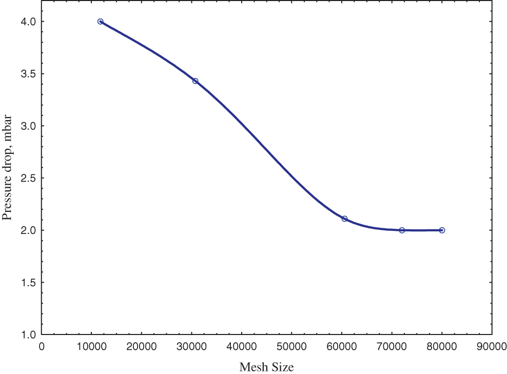
Figure 1: Mesh sensitivity analysis
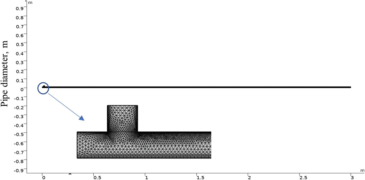
Figure 2: Pipe meshing
The level-set tracking method was introduced by Osher et al. [23]. This method allows the simulation of two immiscible flowing fluids separated by a moving interface. It is advected for a flow field. The function of the level set is a smooth continuous function, denoted as Φ. Two regions were set, for water Φ = 1 and oil Φ = 0. The function changes smoothly, in the transition layer near the interface, from 0 to 1.
The convection equation of the level set function is described as follows [23]:
Changing the fluid parameter at the interface causes a discontinuity in moving parameters which leads to difficulty in the numerical simulation. This difficulty can be overcome by identifying a fixed thickness of the interface where the parameters can change smoothly. However, this method can cause constant interface thickness and mass conservation problems [29]. In the CFD Module of COMSOL Multiphysics®, the following level-set equation is solved [30]:
In this equation, the motion of the interface is represented by the left part of the equation, while the numerical stabilization and reinitialization are defined on the right side. Parameter ε controls the thickness of the interface and parameter
The following Naiver-Stokes equations were solved:
The density as well as the dynamic viscosity are expressed by the following equations:
In which that ρ1 and ρ2 represent the density of fluid 1 and 2, respectively, while μ1 and μ2 are the viscosity of fluid 1 and 2, respectively. In this work, fluid 1 is water and fluid 2, is oil.
To model the turbulence effect, the standard k-ε model and realizability constraints were used. This type of model is very common in industrial applications because of its good convergence rate and relatively low memory requirements. In this model, two variables are solved k which is the turbulence kinetic energy; and the rate of dissipation of turbulence kinetic energy ε (epsilon). Wall functions were used to model the flow close to walls.
The turbulent viscosity can be calculated from the following equation:
In which Cμ represents the model constant
The transport equation (k) is written as:
where pk is the production term and shown as follows:
The transport equation (ε) is written as:
The constant values in the above equations were specified as follows:
Cμ = 0.09, Cε1 = 1.44, Cε2 = 1.92, σk = 1.00 and σε = 1.30, which are the standard values for homogeneous systems.
The turbulent intensity (IT) and the turbulent length (LT) were calculated according to the following equations:
The numerical procedure employs pressure and velocity as the main flow variables. The numerical simulation Multiphysics interface solves the Navier-Stokes equations for the conservation of momentum and a continuity equation for the conservation of mass using the finite element method. The interface position is tracked by solving a transport equation for the level-set function. These equations were solved with the integrated PARDISO solver. The pressure-velocity coupling was discretized by the P2 + P2 scheme and the level-set variables were discretized with quadratic elements. A generalized alpha method with automatic time-step selection was used as the time-step algorithm. The Navier-Stokes and level set equations were solved with a fully coupled approach. The temporal resolution of the result dataset was 0.1 s.
A purchased water-soluble polymer (polyethylene oxide) (MW 8 × 10⁶, density 1.21 g/mL at 25°C, China) was used to prepare the test solution by adding the desired weight to dissolve in distilled water and stirring continuously for 4 h with a magnetic stirrer. The final solution that has a polymer concentration of 150 ppm was left for 24 h to allow maximum penetration of the polymer.
The experiments were carried out in a 3 m length of acrylic horizontal pipe with an inner diameter of 12.7 mm. The schematic diagram of the experimental setup is shown in Fig. 3.
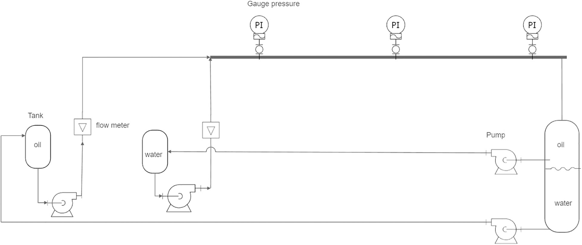
Figure 3: The experimental set-up
All the experiments were carried out under 1 atm and 25°C. The liquids used in the experiments were water and oil (viscosity at 5.5 cp, density 828 kg/m3, surface tension 27.5 mN/m, AL-Dura Refinery). Polyethylene oxide with 150 ppm concentration was added to water as a drag reducer.
The experiments were done under total mixture velocities of 2.3 m/s and four values of water to oil fraction (0.3, 0.4, 0.5, and 0.7). The oil flows in the pipe at the beginning of the experiment for a few seconds, to ensure the wall wettability of the pipe with oil. After, the water fraction was pumped from the storage tank to the test region through a T-junction to ensure proper mixing. The values of pressure were recorded for each meter along the pipe. For certainty, the experiment was repeated two to three times and the average measurement value was adopted.
The variation of pressure drop of two-phase flow water-oil with and without the polymer additive across a pipeline with an increasing volume fraction of water is shown in Figs. 4–7. It can be noticed that as the water fraction increased from 0.3, 0.4, 0.5, and 0.7 the pressure drops increased both with and without polymer addition. This can be explained by the dual effect of increasing superficial water velocity with decreasing superficial oil velocity. This can be explained that at the beginning with low water fraction and higher oil velocity, oil occupies a large part of the cross-section of the pipe, and hence the contribution of the two-phase pressure drop is more predominate, especially the wall of the pipe is wetted by oil. As the water fraction increase, the water-wetted perimeter increases inside the pipe, and this will enhance the turbulence causing to lower pressure drop [10,31–32].
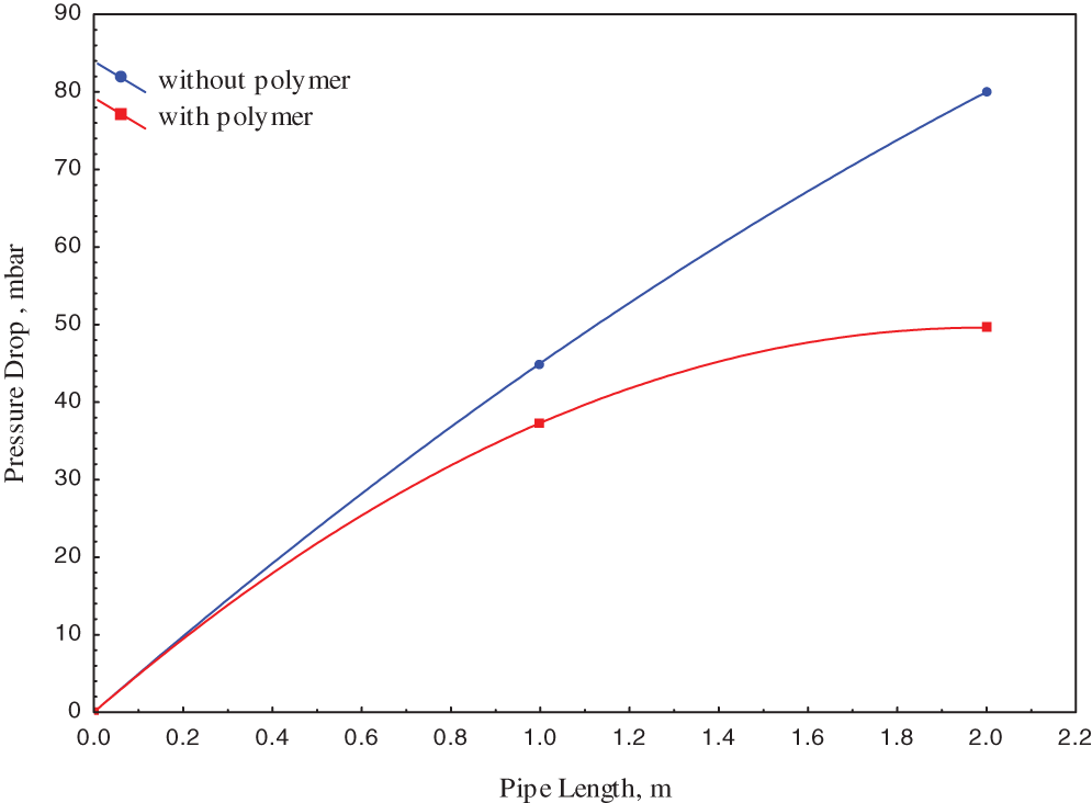
Figure 4: Pressure drop along the pipe with and without the addition of polymer at the water-to-oil ratio of 0.3

Figure 5: Pressure drop along the pipe with and without the addition of polymer at the water-to-oil ratio of 0.4
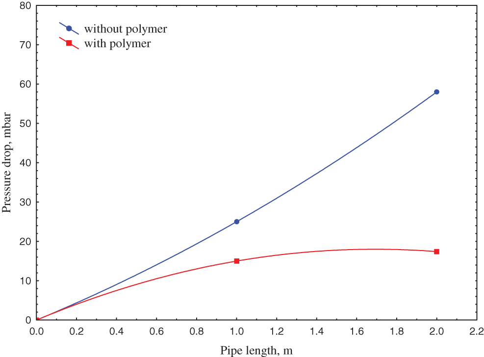
Figure 6: Pressure drop along the pipe with and without the addition of polymer at the water-to-oil ratio of 0.5

Figure 7: Pressure drop along the pipe with and without the addition of polymer at the water-to-oil ratio of 0.7
Indeed, those figures observed that the pressure drop decreases with the polymer addition, in which the pressure drop values reduced to 50, 33, 21, and 17 mbar after polymer addition for water fractions of 0.3, 0.4, 0.5, and 0.7, respectively.
The polymer effect is expressed in terms of the drag-reduction (DR) which can be defined as:
In which that ΔPwithout polymer and ΔPwith polymer represent the measured pressure drop values before and after the addition of polymer, respectively.
According to the above equation, the addition of the polymer effect can be shown in Fig. 8. The figure shows that the drag reduction changed with the changing of water to oil ratio, in which it increased from 0.38, 0.56, and 0.65 to 0.7 with water fractions 0.3, 0.4, 0.5, and 0.7, respectively.
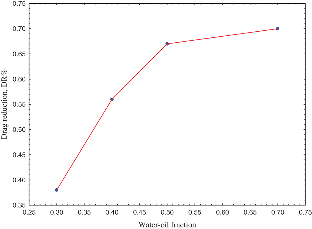
Figure 8: The drag reduction with water-oil fraction
This can be explained by the addition of polymer, at low water fraction which is a stratified water layer as will be shown in the next paragraph, the reduction of the pressure gradient is due to the wall shear stress reduction and interfacial shear reduction between oil and water. On the other hand, the addition of polymer helps to suppress the formation and propagation of the eddies which lead to inhibit the turbulence effect [15] and its effect be more significant with the increasing water fraction, where the water is more dominant than oil and this will enhance droplets coalescence rate and a gravity force dominates leading to stratification of the water phase.
This result is in a line with the work of Abubakar et al. [31] that revealed the increasing oil input fraction resulted in a decrease in drag reduction values. They also reported a zero as well as negative drag reduction at higher values of oil input fraction, while they reported a 64% drag reduction at high mixture velocity and low oil input fraction.
4.2 Volume Fraction Distribution
The radial distribution of the water fraction with/without polymer addition for all water-to-oil velocity ratios after the 1-m pipe entrance is shown by the contour graph as shown in Figs. 9–12. The figures show an interface high difference between the middle and the wall of the pipe. This interface height increases with increasing water-to-oil velocity ratio as expected. However, with polymer addition, a decrease in interface and oil fraction was observed for water to oil velocity ratio. This is due to the reduction of water flow frictional resistance which increases its velocity [33]. However, increasing the ratio to 0.7 a reduction in water fraction was observed, this can be attributed to the increase in damping of the interfacial wave and the drops coalescence that led to an increase of the continuous water layer. Al-Yaari et al. showed similar results that adding polymer caused an increase in the interface height [33].
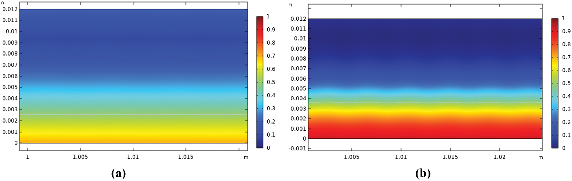
Figure 9: Radial distribution (x-axis) of the water volume fraction (y-axis) at the water-to-oil ratio of 0.3 (a) without polymer (b) with polymer
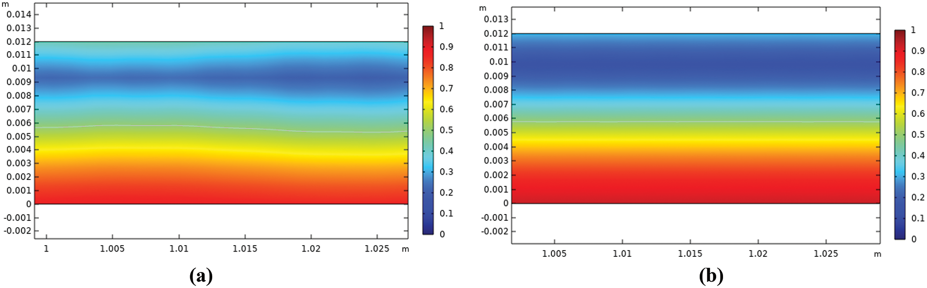
Figure 10: Radial distribution (x-axis) of the water volume fraction (y-axis) at a water-to-oil ratio of 0.4 (a) without polymer (b) with polymer
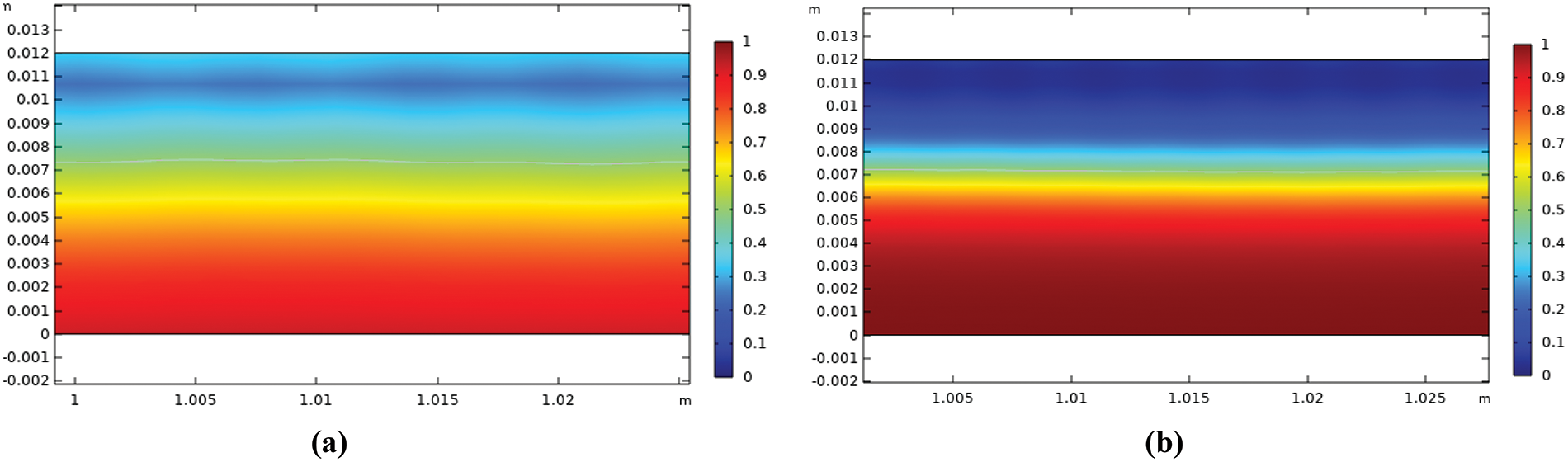
Figure 11: Radial distribution (x-axis) of the water volume fraction (y-axis) at the water-to-oil ratio of 0.5 (a) without polymer (b) with polymer
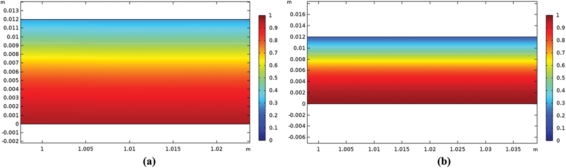
Figure 12: The radial distribution (x-axis) of the water volume fraction (y-axis) at the water-to-oil ratio of 0.7 (a) without polymer (b) with polymer
On the other hand, according to the values of fraction, the water wave is near the pipe bottom due to gravity, and oil drops floated near the top of the pipe. By adding the polymer to the water phase, the characterization of the flow pattern and their transition boundaries changed, in which the wave clarity is observed with polymer addition for all water to oil fractions. The clarity of the wave also increases with increasing water velocity; this agrees with the increase in average water velocity after polymer addition as discussed above.
Figs. 13–16 show the velocity profile of the mixture at different water fractions (0.3, 0.4, 0.5, and 0.7) with and without the addition of polymer which was plotted at pipe cross sections of (0.2, 0.5, 1, and 2 m) from the pipe inlet.
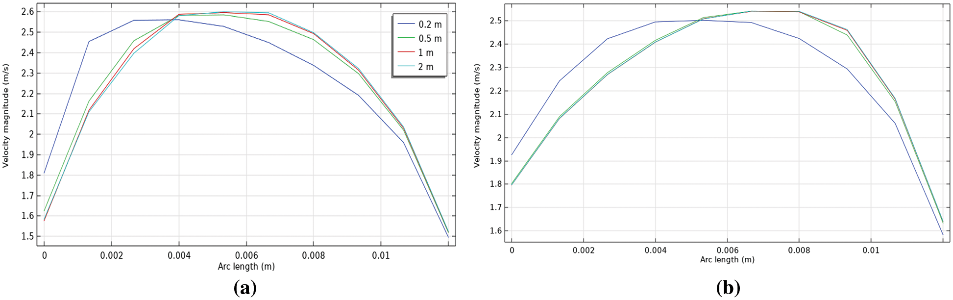
Figure 13: Radial water velocity profile at different distances along the pipe and the water-to-oil ratio of 0.3 (a) without polymer (b) with polymer
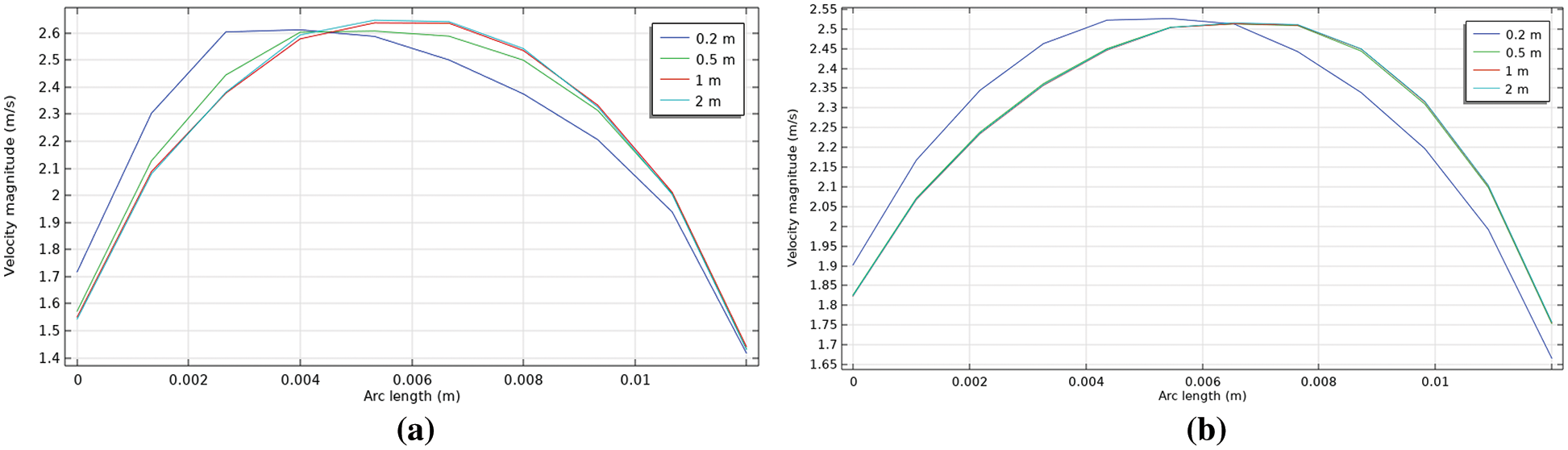
Figure 14: Radial water velocity profile at different distances along the pipe and the water-to-oil ratio of 0.4 (a) without polymer (b) with polymer
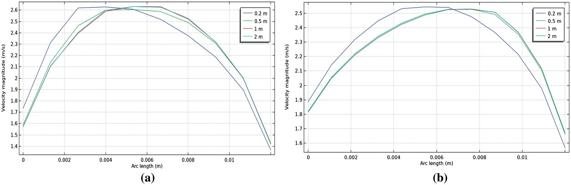
Figure 15: Radial water velocity profile at different distances along the pipe and the water-to-oil ratio of 0.5 (a) without polymer (b) with polymer
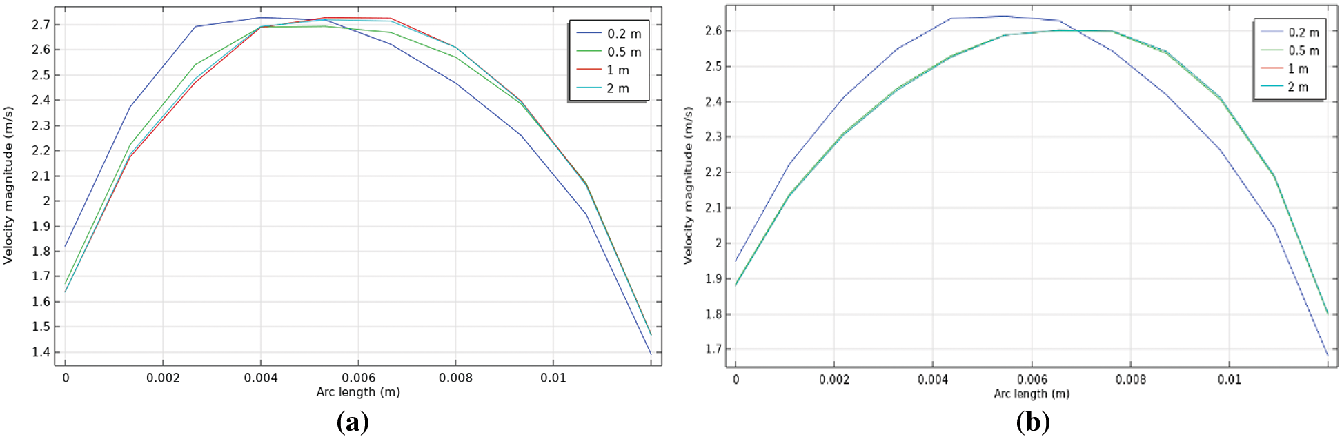
Figure 16: Radial water velocity profile at different distances along the pipe and the water-to-oil ratio of 0.7 (a) without polymer (b) with polymer
The figures show that the velocity is constant at the pipe core and is lower at the pipe wall due to the no-slip boundary condition. Also, the full velocity profile developed after a 0.2 m length distance from the pipe inlet. Indeed, the presence of polymer significantly changed the behavior of the velocity distribution in which that full distribution appears after the polymer addition. The velocity values increase at the wall with the addition of polymer for all oil fractions, for example, it is increased from 1.75 to 1.9 m/s at an oil fraction of 0.5 and section of 0.2 m. This can be attributed to the water layer in the bottom of the pipe, as discussed before, and adding polymer to this layer led to a reduction in friction force causing an increase in the velocity value. On the other hand, the velocity values decrease at the core of the pipe with polymer addition, for example, it decreased from 2.6 to 2.5 m/s at the water-to-oil fraction of 0.3. This is because of the existence of oil layers in the core of the pipe which is less affected by polymer addition. Also, the oil fraction increases did not change the velocity profile.
4.4 Reynolds Number Distribution
The Reynolds stress component of the flow along a 2-m distance from the flow entrance is shown in Figs. 17–20, those figures show that in the case with no polymer addition, the maximum axial velocity profiles increase with a water-oil ratio.
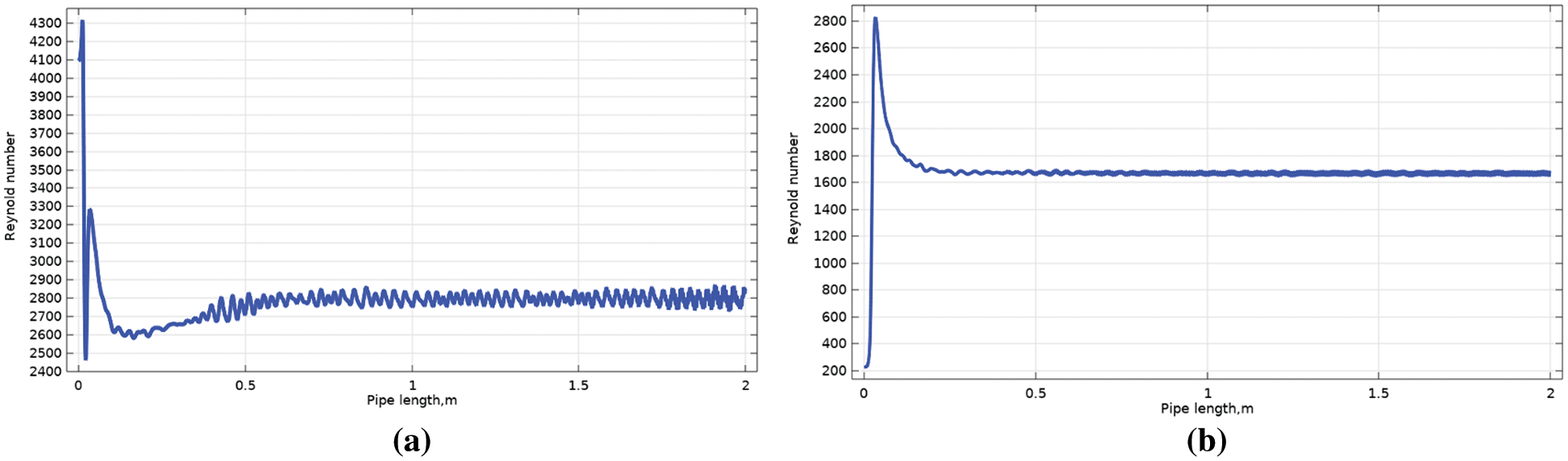
Figure 17: Reynolds number of water along the pipe at the water-oil ratio of 0.3 (a) without polymer (b) with polymer
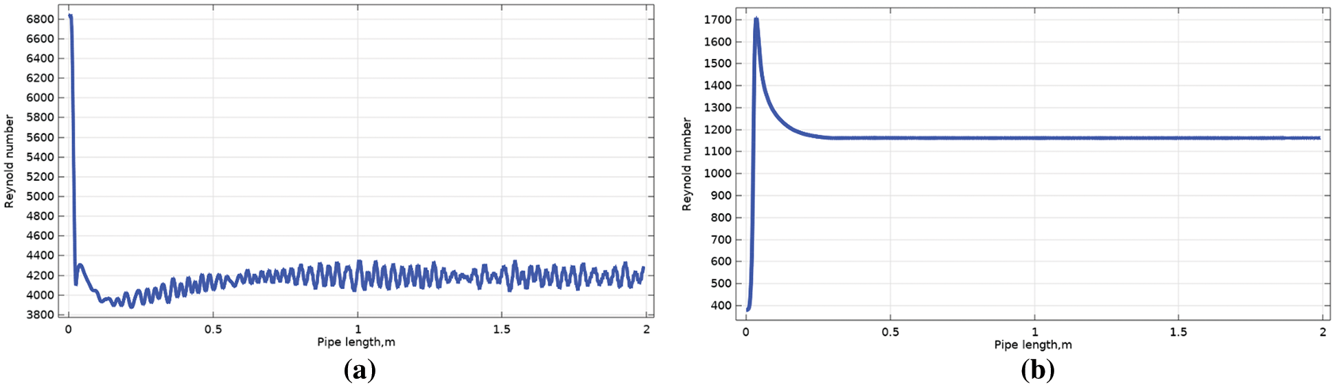
Figure 18: Reynolds number of water along the pipe at the water-oil ratio of 0.4 (a) without polymer (b) with polymer
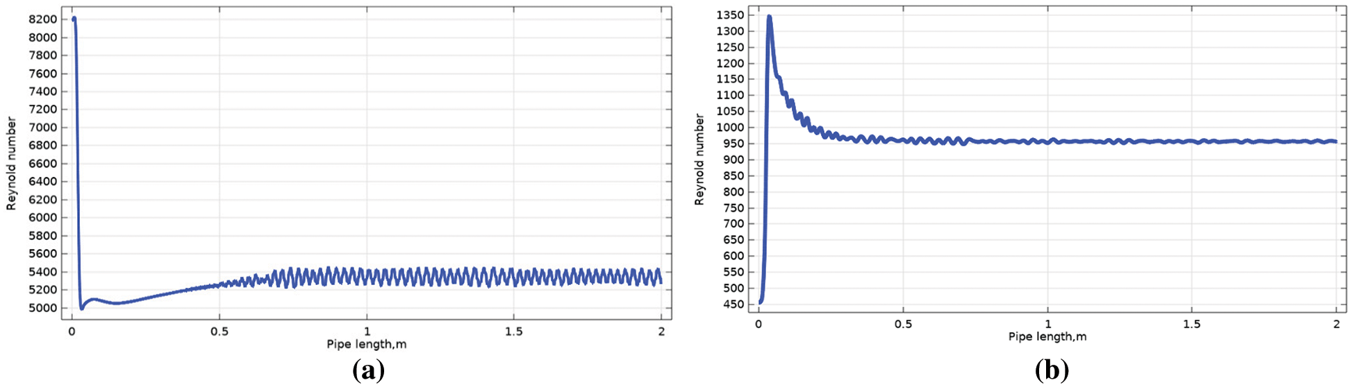
Figure 19: Reynolds number of water along the pipe at the water-oil ratio of 0.5 (a) without polymer (b) with polymer
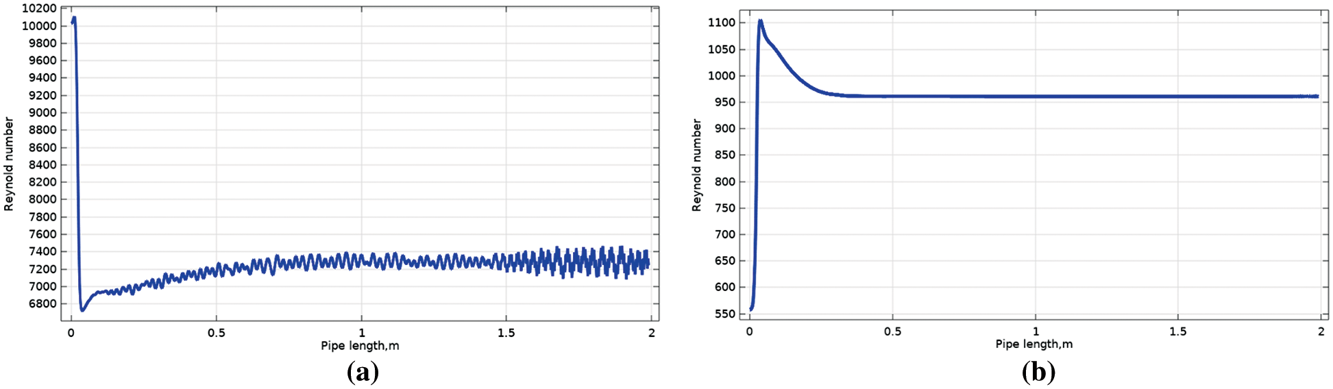
Figure 20: Reynolds number of water along the pipe at the water-oil ratio of 0.7 (a) without polymer (b) with polymer
Indeed, the figures reveal that at water fraction 0.3 the Reynold number increases till 0.6 m distance, and its value has fluctuated along the pipe. The addition of polymer results in reducing Reynolds number fluctuation along the pipe and more significantly near interface regions and its value decrease, for example, from 2600 to 1700 (nearly 35%). Increasing the water fraction, the Reynolds number reduction increased to 70%, 82%, and 87% at water fractions 0.4, 0.5, and 0.7, respectively. This indicates that the effect of the polymer as a drag reducer is clearer at high values of the water fraction.
This reduction directs to the turbulent momentum transfer decreasing in the radial direction [34,35]. It is well known that turbulent eddies are formed from the high-velocity gradients near-wall region. Those eddies are transported into the bulk flow of the pipe in the radial direction in contradiction to the desired axial flow direction. This results in energy losses and an increase in pressure drop. With the addition of polymer, the reduction of eddies leads to a decrease in energy loss.
The model validation can be expressed in Fig. 21 which shows a comparison between the experimental pressure drops across the pipe and the predicted values from the model. The figure shows good agreement between the experimental and the predicted value with an error of less than 7%.
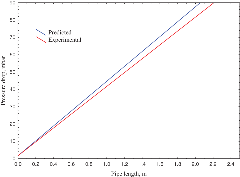
Figure 21: The experimental and predicted values of pressure drop along the pipe of the water-oil ratio of 0.3 without polymer
In this study, the effect of polyethylene oxide on the pressure drop of oil-water flows in a horizontal acrylic pipe was experimentally investigated and simulated using the COMSOL software. The results show the following conclusions:
• In all water-oil ratios, polymers’ addition affected the flow pattern and its transition. Overall, adding polymer increased the range of oil superficial velocity and flow clarity of the two phases and this clarity appeared more with increasing water fraction.
• The pressure drop reduction differed at the various is related to the superficial velocity of the phases, i.e., water fraction. The largest drag reduction value was 70% at a water fraction of 0.7.
• The drag reductions generally increased with water fraction and reduced with oil fraction in the region of strong turbulence. Reynolds number: Increasing the water fraction, the Reynolds number reduction increased to 70, 82, and 87% at water fractions 0.4, 0.5, and 0.7, respectively.
• The level set model as well as the k-ε turbulence model show a reasonable phase distribution for the oil/water flow patterns. Quantitatively, the maximum pressure drop deviation between experimental and simulated values was 7%. This confirms that the presented model can describe well this type of two/phase flow.
Acknowledgement: The authors would like to thank the Chemical Engineering Department at the University of Technology for as well as Department of Chemical Engineering and Petroleum Industries at the Al-Mustaqbal University College for their support.
Funding Statement: The authors received no specific funding for this study.
Conflicts of Interest: The authors declare that they have no conflicts of interest to report regarding the present study.
References
1. Hasan, S. W., Ghannam, M. T., Esmail, N. (2010). Heavy crude oil viscosity reduction and rheology for pipeline transportation. Fuel, 89, 1095–1100. [Google Scholar]
2. Al-Yaari, M., Soleimani, A., Abu-Sharkh, B., Al-Mubaiyedh, U., Al-Sarkhi, A. (2009). Effect of drag-reducing polymers on oil-water flow in a horizontal pipe. International Journal of Multiphase Flow, 35(6), 516–524. https://doi.org/10.1016/j.ijmultiphaseflow.2009.02.017 [Google Scholar] [CrossRef]
3. Martinez-Palou, R., Mosqueira, M., Zapata-Rendón, B., Mar-Juárez, E., Bernal-Huicochea, C. et al. (2011). Transportation of heavy and extra-heavy crude oil by pipeline: A review. Journal of Petroleum Science and Engineering, 75(3–4), 274–282. https://doi.org/10.1016/j.petrol.2010.11.020 [Google Scholar] [CrossRef]
4. Santos, R., Brinceno, M., Loh, W. (2017). Laminar pipeline flow of heavy oil-in-water emulsions produced by continuous in-line emulsification. Journal of Petroleum Science and Engineering, 156(5), 827–834. https://doi.org/10.1016/j.petrol.2017.06.061 [Google Scholar] [CrossRef]
5. Hart, A. (2014). A review of technologies for transporting heavy crude oil and bitumen via pipelines. Journal of Petroleum Exploration and Production Technology, 4(3), 327–336. https://doi.org/10.1007/s13202-013-0086-6 [Google Scholar] [CrossRef]
6. Alsaedi, S. S., Yousif, Z., Filip, P. (2020). The impact of adding titanium oxide to polyethylene oxide to improve drag reduction percentage using a closed-loop recirculation system. Solid State Technology, 63(1), 860–866. [Google Scholar]
7. Alwasiti, A. A., Shneen, Z. Y., Ibrahim, R. I., Shalal, A. A. (2021). Energy analysis and phase inversion modeling of two-phase flow with different additives. Ain Shams Engineering Journal, 12(1), 799–805. https://doi.org/10.1016/j.asej.2020.07.004 [Google Scholar] [CrossRef]
8. Kamel, A. H., Shah, S. N. (2013). Maximum drag reduction asymptote for surfactant-based fluids in circular coiled tubing. Journal of Fluids Engineering, 135(3), 031201-1. https://doi.org/10.1115/1.4023297 [Google Scholar] [CrossRef]
9. Shnain, Z. Y., Alwasiti, A. A., Rashed, M. K., Shakor, Z. M. (2022). Experimental and data-driven approach of investigating the effect of parameters on the fluid flow characteristic of nanosilica enhanced two phase flow in pipeline. Alexandria Engineering Journal, 61(2), 1159–1170. https://doi.org/10.1016/j.aej.2021.06.017 [Google Scholar] [CrossRef]
10. Manfield, C. J., Lawrence, C., Hewitt, G. (1999). Drag-reduction with additive in multiphase flow: A literature survey. Multiphase Science Technology, 11(3), 197–221. https://doi.org/10.1615/MultScienTechn.v11.i3.20 [Google Scholar] [CrossRef]
11. Warwaruk, L., Ghaemi, S. (2021). A direct comparison of turbulence in drag-reduced flows of polymers and surfactants. Journal of Fluid Mechanics, 917, A7. https://doi.org/10.1017/jfm.2021.264 [Google Scholar] [CrossRef]
12. Edomwonyi-Out, L. C., Simeoni, M., Angeli, P., Campolo, M. (2016). Synergistic effect of drag reducing agents in pipes of different diameters. Nigerian Journal of Engineering, 22, 1–5. [Google Scholar]
13. Al-Wahaibi, T., Smith, S., Angeli, P. (2007). Effect of drag-reducing polymers on horizontal oil water flows. Journal of Petroleum Science and Engineering, 57(3–4), 334–346. https://doi.org/10.1016/j.petrol.2006.11.002 [Google Scholar] [CrossRef]
14. Edomwonyi-Out, L. C., Angeli, P. (2019). Separated oil-water flows with drag reducing polymers. Experimental Thermal and Fluid Science, 102(1604), 467–478. https://doi.org/10.1016/j.expthermflusci.2018.12.011 [Google Scholar] [CrossRef]
15. Edomwonyi-Out, L. C., Gimba, M. M., Yusuf, N. (2020). Drag reduction with biopolymer-synthetic polymer mixtures in oil-water flows: Effect of synergy. Engineering Journal, 24(6), 1–10. https://doi.org/10.4186/ej.2020.24.6.1 [Google Scholar] [CrossRef]
16. Liu, D., Wang, S., Ivitskiy, I., Wei, J., Tsui, O. et al. (2021). Enhanced drag reduction performance by interactions of surfactants and polymers. Chemical Engineering Science, 232, 116336. https://doi.org/10.1016/j.ces.2020.116336 [Google Scholar] [CrossRef]
17. Dai, X., Li, B., Li, L., Yin, S., Wang, T. (2021). Experimental research on the characteristics of drag reduction and mechanical degradation of polyethylene oxide solution. Energy Sources, Part A: Recovery, Utilization, and Environmental Effects, 43(8), 944–952. https://doi.org/10.1080/15567036.2019.1632988 [Google Scholar] [CrossRef]
18. Sosa, J., Urquiza, G., Garcia, J., Castro, L. (2015). Computational fluid dynamics simulation and geometric design of hydraulic turbine draft tube. Advances in Mechanical Engineering, 7(10), 168781401560630. https://doi.org/10.1177/1687814015606307 [Google Scholar] [CrossRef]
19. Maakala, V., Jarvinen, M., Vuorinen, V. (2018). Computational fluid dynamics modeling and experimental validation of heat transfer and fluid flow in the recovery boiler superheater region. Applied Thermal Engineering, 139(5), 222–238. https://doi.org/10.1016/j.applthermaleng.2018.04.084 [Google Scholar] [CrossRef]
20. Tao, J., Sun, Q., Liang, W., Chen, Z., He, Y. et al. (2018). Computational fluid dynamics based dynamic modeling of parafoil system. Applied Mathematical Modelling, 54, 136–150. https://doi.org/10.1016/j.apm.2017.09.008 [Google Scholar] [CrossRef]
21. Blunt, M. J. (2001). Flow in porous media, pore-network models and multiphase flow. Current Opinion in Colloid & Interface Science, 6(3), 197–207. https://doi.org/10.1016/S1359-0294(01)00084-X [Google Scholar] [CrossRef]
22. Unverdi, S. O., Tryggvason, G. (1992). A front tracking method for viscous, incompressible, multiphase flows. Journal of Computational Physics, 100(1), 25–37. https://doi.org/10.1016/0021-9991(92)90307-K [Google Scholar] [CrossRef]
23. Osher, S. J., Sethian, J. A. (1988). Front propagating with curvature dependent speed: Algorithms based on Hamilton-Jacobi formulations. Journal of Computational Physics, 79(1), 12–49. https://doi.org/10.1016/0021-9991(88)90002-2 [Google Scholar] [CrossRef]
24. Smereka, P., Sethian, J. A. (2003). Level set methods for fluid interfaces. Annual Review of Fluid Mechanics, 35(1), 341–372. https://doi.org/10.1146/annurev.fluid.35.101101.161105 [Google Scholar] [CrossRef]
25. Jacqmin, D. (1999). Calculation of two-phase Navier-Stokes flows using phase field modeling. Journal of Computational Physics, 155(1), 96–127. https://doi.org/10.1006/jcph.1999.6332 [Google Scholar] [CrossRef]
26. Badalassi, V. E., Cenicerob, H. D., Banerjee, S. (2003). Computation of multiphase systems with phase field models. Journal of Computational Physics, 190(2), 371–397. https://doi.org/10.1016/S0021-9991(03)00280-8 [Google Scholar] [CrossRef]
27. Sussman, M., Almgren, A. S., Bell, J. B., Colella, P., Howell, L. H. et al. (1999). An adaptive level set approach for incompressible two-phase flows. Journal of Computational Physics, 148(1), 81–124. https://doi.org/10.1006/jcph.1998.6106 [Google Scholar] [CrossRef]
28. Yue, P., Zhou, C., Feng, J. J., Ollivier-Gooch, C. F., Hu, H. H. (2006). Phase-field simulations of interfacial dynamics in viscoelastic fluids using finite elements with adaptive meshing. Journal of Computational Physics, 219(1), 47–67. https://doi.org/10.1016/j.jcp.2006.03.016 [Google Scholar] [CrossRef]
29. Ferziger, J. (2003). Interfacial transfer in Tryggvason’s method. International Journal for Numerical Methods in Fluids, 41(5), 551–560. https://doi.org/10.1002/(ISSN)1097-0363 [Google Scholar] [CrossRef]
30. COMSOL AB (2012). COMSOL multiphysics reference guide (version 4.3). Stockholm, Swede. [Google Scholar]
31. Abubakar, A., Al-Wahaibi, T., Al-Hashmi, A. R., Al-Wahaibi, Y., Al-Ajmi, A. et al. (2015). Influence of drag-reducing polymer on flow patterns, drag reduction and slip velocity ratio of oil-water flow in horizontal pipe. International Journal of Multiphase Flow, 73, 1–10. https://doi.org/10.1016/j.ijmultiphaseflow.2015.02.016 [Google Scholar] [CrossRef]
32. Al-Sarkhi, A. (2010). Drag reduction with polymers in gas-liquid/liquid-liquid flows in pipes: A literature review. Journal of Natural Gas Science and Engineering, 2(1), 41–48. https://doi.org/10.1016/j.jngse.2010.01.001 [Google Scholar] [CrossRef]
33. Al-Yaari, M., Al-Sarkhi, A., Abu-Sharkh, B. (2012). Effect of drag reducing polymers on water holdup in an oil-water horizontal flow. International Journal of Multiphase Flow, 44, 29–33. https://doi.org/10.1016/j.ijmultiphaseflow.2012.04.001 [Google Scholar] [CrossRef]
34. Gyr, A., Tsinober, A. (1997). On the rheological nature of drag reduction phenomena. Journal of Non-Newtonian Fluid Mechanics, 73(1–2), 153–162. https://doi.org/10.1016/S0377-0257(97)00055-4 [Google Scholar] [CrossRef]
35. Yu, B., Li, F., Kawaguchi, Y. (2004). Numerical and experimental investigation of turbulent characteristics in a drag-reducing flow with surfactant additives. International Journal of Heat and Fluid Flow, 25(6), 961–974. https://doi.org/10.1016/j.ijheatfluidflow.2004.02.029 [Google Scholar] [CrossRef]
Cite This Article
 Copyright © 2023 The Author(s). Published by Tech Science Press.
This work is licensed under a Creative Commons Attribution 4.0 International License , which permits unrestricted use, distribution, and reproduction in any medium, provided the original work is properly cited.
 Downloads
 Citation Tools