Optimized Design of H-Type Vertical Axis Wind Airfoil at Multiple Angles of Attack

1  Introduction

With the rapid development of modern wind power generation technology, the use of wind energy has become one of the pillars of modern clean energy, and is an important solution to alleviating the fossil energy crisis and environmental pollution on an international scale. Compared with horizontal axis wind turbines, vertical axis wind turbines do not require complex guides, their manufacturing and installation costs are lower, the blade tip speed ratio is low during operation, and the noise is small. Due to the low utilization rate of wind energy, vertical axis wind turbines are not widely manufactured and applied. As the core component of vertical axis wind turbines, improving the aerodynamic performance of wind turbine blades is an effective means to improve the utilization rate of wind energy of wind turbines.

With the aim of improving on the aerodynamic characteristics of vertical axis wind turbine blades, scholars and experts have carried out a lot of research and exploration. Liu et al. [1] studied the key parameters such as torque, power coefficient, and tangential force of the four-blade vertical axis wind turbine by using the separation vortex simulation (DES) method, and the results showed that the DES scheme is a suitable method to study the hybrid vertical axis wind turbines’ (HVAWT) performance, and which was verified by the flow field including instantaneous torque and vortex shedding. Baghdadi et al. [2] used Bernstein polynomials to complete the optimization design of the vertical axis wind turbine blade section airfoil, and simulated the aerodynamic performance of the optimized airfoil, and the simulation results show that this method can achieve the optimization of the airfoil. Li et al. [3] used the optimized and improved HICKS-HERNNE type function to fit the contour of the S8035 airfoil curve, and combined it with the multi-objective particle swarm algorithm to realize the optimal design of the airfoil curve. The aerodynamic performance of the optimized airfoil is simulated and verified by XFOIL software, and the results show that the aerodynamic performance of the optimized airfoil is improved. Based on the particle swarm optimization algorithm, Ma et al. [4,5] proposed a combinatorial optimization design method for wind turbine blades. The optimized wind turbine blades significantly increase in power under low and medium wind speeds and obtain better anti-fatigue performance. Rezaeiha et al. [6] studied the influence of different pitch angles of vertical axis wind turbines on the wind energy utilization rate of vertical axis wind turbines, and the results showed that the wind turbine performance was best when the slurry pitch angle of the wind turbine blades was −2°. Amine et al. [7] to improve the aerodynamic performance of the vertical axis wind turbine, combined computational fluid dynamics (CFD) and a user defined function (UFD) to analyze the dynamic pitch motion and plasma effect of the wind turbine blade. The results show that by applying the dielectric barrier discharges (DBD) plasma drive, the power coefficient of the wind turbine is increased by 8%. Song et al. [8] pointed out that the influencing factors of the aerodynamic characteristics of vertical axis wind turbines have not been paid attention to in the past, and this paper calculates the aerodynamic performance of wind turbines through CFD technology, and obtains the airfoil thickness of optimized airfoils between 15%–18%. Celik et al. [9] evaluated the self-starting behavior of H-type vertical axis wind turbine by establishing a CFD starting model of the turbine. The results show that an increase in the number of blades will make it easier for the wind turbine to start, which may lead to a decrease in the power coefficient of the wind turbine.

The applied research on improving the wind energy utilization rate of vertical axis wind turbines is performed by changing the shape of airfoils under a single angle of attack. But, because the distribution of wind fields is extremely complex and the range of attack angles of vertical axis wind turbines during operation is large, the research on a single angle of attack cannot fully improve the wind energy utilization rate of vertical axis wind turbines. In this paper, the optimal design of the vertical axis wind turbine blade airfoil is realized within a certain angle of attack, the NACA 2412 airfoil is used as the original airfoil, the aerodynamic shape characteristics of the airfoil are characterized by the Bézier curve function, and the vertical axis wind turbine blade is optimized by the moving asymptotic algorithm coupled with XFOIL software. According to the power coefficient, moment coefficient, speed and pressure distribution diagram of the wind turbine before and after optimization, the optimization results of the vertical axis wind turbine are analyzed and compared.

2  Parametric Characterization of Airfoil Curves

To better characterize the airfoil profile curve, the third Bézier curve function is used to parametrically characterize the aerodynamic shape of the airfoil. According to [10] the general expression of its polynomial function of degree n is as follows:

P(t)=∑i=0n⁡PiBi,n(t)t∈[0,1];i=0,1,2⋯n  (1)

where ( Bi,n(t) ) is:

Bi,n(t)=n!i!⋅(n−i)!⋅ti⋅(1−t)n−1   t∈[0,1];i=0,1,2⋯n (2)

where: Bi,n(t) is the n-th basis function; Pi is the position vector of each node in the curve; t is the abscissa of Bézier curve.

The parametric expressions of the upper and lower surfaces of the airfoil of the vertical axis wind turbine blade section are:

Upper airfoil ( ϑU ):

ϑu(xt)=C(xt)⋅Su(xt)+xt⋅Δϑu (3)

Lower wing surface ( ϑl ):

ϑl(xt)=C(xt)⋅Sl(xt)+xt⋅Δϑl (4)

where: C(xt) is a class function; xt=x/c is the dimensionless coordinate of the airfoil in the x direction; Su(xt) , Sl(xt) is the shape contour function; xt⋅Δϑu , xt⋅Δϑl is the trailing edge thickness, Δϑ=yTE/c ; c is the chord length of the airfoil, and c=1 .

Therefore, the type function expression of the airfoil is:

C(xt)=xtN1⋅(1−xt)N2  (5)

where: N1=0.5;N2=0.1 .

In the third order Bézier curve parametric expression, the third order parametric curve expression of Bi,n(t) is:

B0,3(t)=(1−t)2⋅B0+2t⋅(1−t)⋅B1+3t2⋅(1−t)⋅B2+t3⋅B3   [0,1]  (6)

The matrix form is:

M(xt)=B0,3(t)= [t3t2t1][−133−6−3130−33100000][B0B1B2B3] (7)

where: Point B0, B1, B2, B3 is to optimize fixed control points for airfoils on Bézier curves.

In this paper, the NACA 2412 airfoil is taken as the original airfoil, and its aerodynamic shape is fitted by using the third-order Bessel curve function. The fitting curve of the NACA 2412 airfoil is shown in Fig. 1.

Figure 1: NACA 2412 airfoil fitting curve

In this work, to better control the shape of the upper and lower airfoil surfaces, the control points P0, P1, P2 and P3 are set along the X-axis, and the boundaries of each control point along the X-axis direction range are 0≤P0,x≤20; 20≤P1,x≤40 ; 60≤P2,x≤80 ; 80≤P3,x≤100 . The fitted values for each control point are shown in Table 1.

3  H-Type Vertical Axis Wind Airfoil Optimization Design

3.1 Moving Asymptotic Algorithm

The method of moving asymptote algorithm (MMA) [11] solves the original problem by using its many subproblems. Its general mathematical model of the subproblem is:

minf0(xn)+a0+∑i=1m⁡(yici+12diyi2)

s.t.fi(xn)−aiz−yi≤0    i=1,2,⋯,I

αjn≤xj≤βjn                  j=1,2,⋯,J+1 (8)

where: f0(xn) , fi(xn) is a convex function; yi , z is an additional variable and satisfies yi ≥ 0, z ≥ 0; αjn, βjn are the upper bound and lower bound of the constraint variable, respectively; I is the number of constraints; J is the number of design variables.

The values of αjn,βjn are:

αjn=max{xjmin,Ljn+0.1(xjn−Ljn),xjn−0.5(xjmax−xjmin)} (9)

βjn=min{xjmax,Ujn−0.1(Ujn−xjn),xjn+0.5(xjmax−xjmin)}  (10)

The expression of fin(x) is:

fin(x)=rin+∑i=1m⁡(pijnUjn−xj+qijnxj−Ljn)  (11)

The  Pijn, Qijn Rik  expressions for and are:

Pijn=(Ujn−xjn)2{1.001(∂fi(xn)∂xj)+ +0.001(∂fi(xn)∂xj)−+10−5xjmax−xjmin} (12)

Qijn=(xjn−Ljn)2{0.001(∂fi(xn)∂xj)++1.001(∂fi(xn)∂xj)−+10−5xjmax−xjmin} (13)

Rik=fi(xn)−∑j=1n⁡(PijnUjn−xjn+Qijnxjn−Ljn)  (14)

where: Ujn, Ljn are the upper asymptote and the lower asymptote of a function; Pijn, Qijn are the sensitivity coefficients of the upper and lower asymptotic; Rin is the undetermined coefficient. The coefficients Pijn, Qijn,Rin and the upper and lower asymptotic Ujn, Ljn are constantly updated with the iterative transformation.

In g the MMA algorithm to solve the optimization problem, in the process of n iterations, the upper limit Ujn and lower limit Ljn of the design variable xj are constantly updated according to the following rules. When n=1 or n=2 :

When n=1 or n=2 :

Ujn=xjn+δ1,2(xjmax−xjmin)

Ljn=xjn−δ1,2(xjmax−xjmin) (15)

where: xjmax,xjmin are the upper boundary and lower boundary of the design variable xj ; xjn is the value of xj after n iterations; δ1,2=0.5 ( 0>δ1,2<1 ).

When n ≥ 3, the positive and negative signs of the values of  (xjn−xjn−1) and (xjn−1−xjn−2) must be considered:

Ujn=xjn+δj(Ujk−1−xjk−1)

Ljn=xjn−δj(xjk−1−Ljk−1) (16)

When 0>δJ<1 , and when the symbols of (xjn−xjn−1) and (xjn−1−xjn−2) are opposite, the variable xj oscillates, making the moving limit close to xjn , and making the MMA approximation more conservative. When the symbols of (xjn−xjn−1) and (xjn−1−xjn−2) are the same, the moving limit is far away from xjn , which makes the MMA converge faster.

When δJ>1 , the design variable  xj must meet the following requirements  αjn≤xj≤βjn , which can effectively prevent the iterative sum from being zero and avoid being divided by zero in the MMA approximation.

3.2 Objective Function, Design Variables and Constraints for Blade Airfoil Optimization

In the optimization design of the H-type vertical axis wind turbine blade airfoil, important parameters such as the curvature of the airfoil, the maximum thickness of the airfoil, and the position of the airfoil curvature and maximum thickness relative to the chord length of the airfoil have a serious impact on the airfoil optimization results. Under the normal working state of low Reynolds number, the attack angle of the blade can be increased within a suitable range, which can improve the lift coefficient. Increasing the thickness of the blades allows the wind turbine to start at lower wind speeds. At the same time, to reduce the number of algorithm iterations and reduce the time cost, the airfoil parameters must be controlled in the process of airfoil optimization.

3.2.1 Objective Function

The research in this paper fully considers the special working mode of the H-type vertical axis wind turbine. When the vertical axis wind turbine operates under normal conditions, the magnitude of the tangential force coefficient Ct of the blade is an important parameter to evaluate the wind energy utilization rate of the vertical axis wind turbine. Therefore, improving the tangential force coefficient of the blade is the primary objective of blade airfoil optimization. In this paper, it is proposed that under the condition of blade airfoil angle of attack, in the low Reynolds number and corresponding Mach number environment, the maximum tangential force coefficient under the blade airfoil angle of attack is the objective function, as α(−10∘≤α≤15∘) shown in Eq. (17).

f(x)=maxCt=max(CLsinα−CDcosα)  (17)

where: Ct is the blade tangential force coefficient; CL is the lift coefficient of blade airfoil; CD is the drag coefficient of blade airfoil; α is the blade airfoil angle of attack.

3.2.2 Design Variables

In the optimization design process of the vertical axis wind turbine blade airfoil, the selection of design variables and the control range of variables have a significant impact on the results of the optimized design. According to the NACA 2412 airfoil curve fitted by the Bézier curve, this paper selects five control parameter points ( PU0,PU1,PU2,PU3,PU4,PL0,PL1,PL2,PL3,PL4 ) for the upper and lower airfoil surfaces of the airfoil curve, respectively. To better control the passivated trailing edge of the airfoil, we set the parameter control point P4 . Its design variable X is:

X=(PU0,PU1,PU2,PU3,PU4,PL0,PL1,PL2,PL3,PL4) (18)

3.2.3 Constraints

In the process of optimizing the design of the blade airfoil, important parameters such as the curvature of the airfoil, the maximum thickness of the airfoil, and the position of the airfoil curvature and the maximum thickness relative to the chord length of the airfoil have a serious impact on the airfoil optimization results. To ensure that the optimized airfoil has good aerodynamic performance and to reduce the time cost of the algorithm iteration, corresponding constraints must be established.

The thickness and curvature of the airfoil is very important to the aerodynamic characteristics of the airfoil and where the thickness of the airfoil is too thin, it may affect the structural strength of the blades. So, the maximum relative thickness of the optimized airfoil should not be less than the original airfoil. The constraints on the relative maximum thickness of the airfoil, the maximum curvature of the airfoil, and the location of the maximum curvature of the airfoil chord length are given in Eqs. (19)–(21).

Constraints on the relative maximum thickness of the airfoil:

0.12≤ tmax ≤0.18,(m)  (19)

Constraints on the maximum curvature of the airfoil:

0%≤ c ≤8%  (20)

Constraints on the position of the airfoil chord length at the maximum curvature of the airfoil:

0.6≤Lmax≤0.9,(m) (21)

3.3 Blade Airfoil Optimization Design Process

The blade airfoil optimization design process mainly includes several main steps, such as parametric characterization of the airfoil, experimental scheme design, meshing, airfoil CFD flow field solution, and airfoil optimization, and all steps are realized through script files in MATLAB software. The flow of blade airfoil optimization design is shown in Fig. 2.

Figure 2: Airfoil optimization design process

3.4 Analysis of Airfoil Curve Optimization Results

A new optimized airfoil is obtained by using the MMA, as shown in Fig. 3. The leading edge of the optimized airfoil is slightly increased, the thickness of the middle and front part of the airfoil is slightly increased, and its tail curvature is also significantly increased. Within the range of attack angle α (−10° ≤ α ≤ 15°), is the curve of the angle of attack of the airfoil drawn and its related parameters.

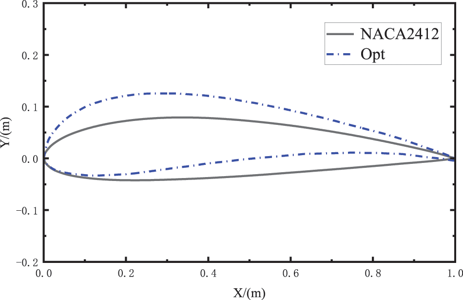
Figure 3: Comparison between the NACA 2412 airfoil and the optimized airfoil

Fig. 4 shows the lift coefficient of the NACA2412 airfoil compared to the optimized airfoil. The lift coefficient gradually increases in the range of angle of attack α(−10∘≤α≤15∘), the lift coefficient of the optimized airfoil exceeds the original airfoil at the corresponding angle of attack, and the maximum lift coefficient of the optimized airfoil exceeds the maximum lift coefficient of the original airfoil by 8.33%.

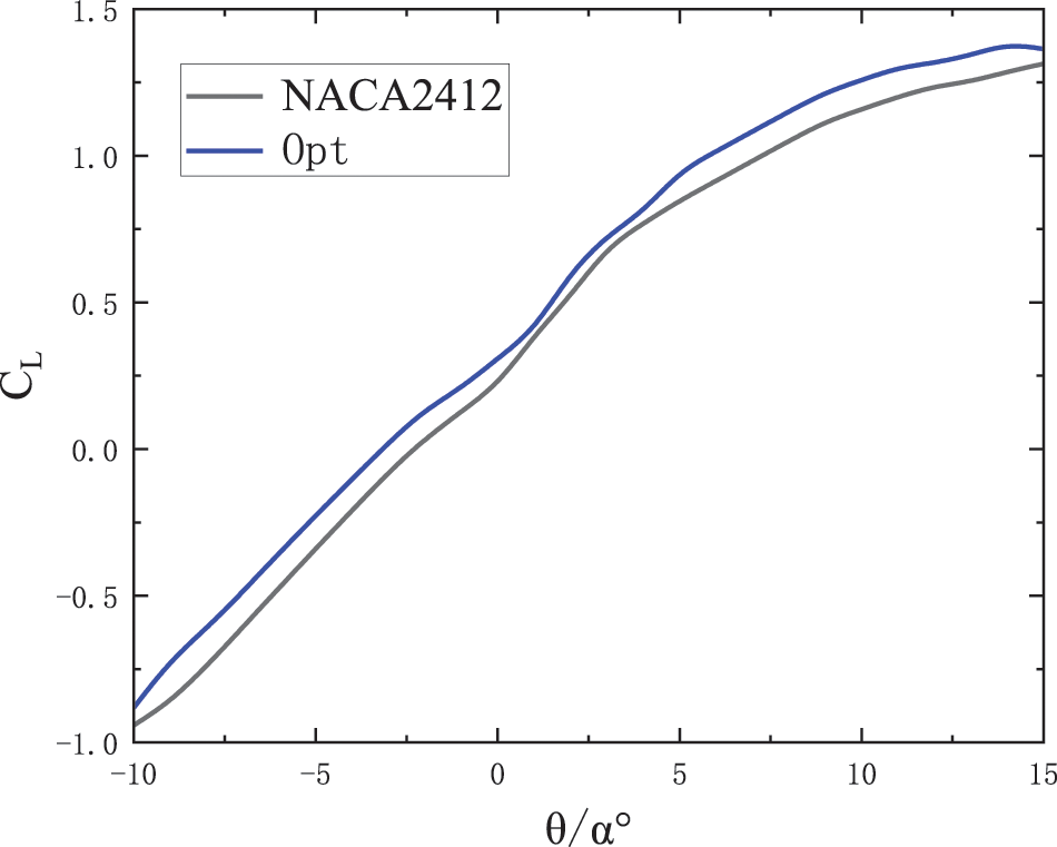
Figure 4: Diagram of the comparison of lift coefficient before and after airfoil optimization

Fig. 5 shows the lift-to-drag ratio of the NACA2412 airfoil and the optimized airfoil. In the range of attack angle α(−10∘≤α≤15∘) , the lift-drag ratio of the optimized airfoil is always higher than that of the original airfoil, and the trend of change of the lift-drag ratio curve is first an increase, and then a decrease, and the lift-drag ratio of the optimized airfoil reaches a maximum when the attack angle of the airfoil is α = 5°, which is 11.22% higher than that of the original airfoil.

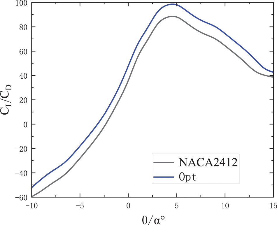
Figure 5: Comparison of the lift drag ratio before and after airfoil optimization

4  H-Type Vertical Axis Wind Airfoil Optimization Verification

4.1 Relevant Parameters of the H-Type Vertical Axis Wind Turbine

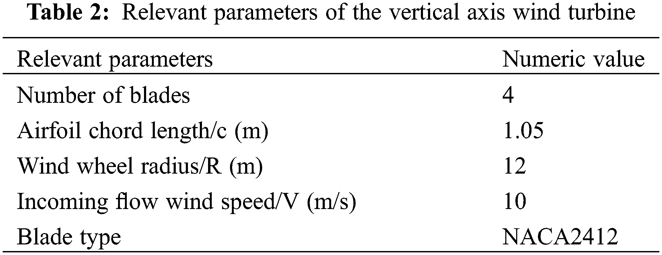
The model parameters of the symmetrical H-type vertical axis wind turbine selected in this paper are shown in Table 2.

4.2 Computational Domains and Meshing

For vertical axis wind turbines, without considering the turbulence at the upper and lower ends of the blades, the flow field around the airfoil in the vertical direction can be approximated, and the three-dimensional flow field can be simplified to a two-dimensional flow field [12]. Therefore, a two-dimensional calculation model is selected for the numerical simulation of the H-type vertical axis wind turbine, and the calculation domain is shown in Fig. 6. The outer basin (1), the rotation domain (2), and the inner basin (3) together form a complete computational domain model. Using the wind tunnel test model of McLaren, [13] as a reference, the outer basin is set to a calculation domain with a length of 50R and a width of 28R. The interface between the outer basin and the rotating domain, the rotational domain and the inner basin, are set as the boundary conditions. The left side of the calculation domain is set to the velocity inlet (Velocity_inlet), and the flow velocity of the calculation domain V = 10 m/s, and the flow velocity direction is from left to right. The right side is set to the pressure outlet (Pressure_Outlet). The upper and lower boundaries are symmetrical boundaries set to (Symmetry). The airfoil boundary is set to a movable boundary.

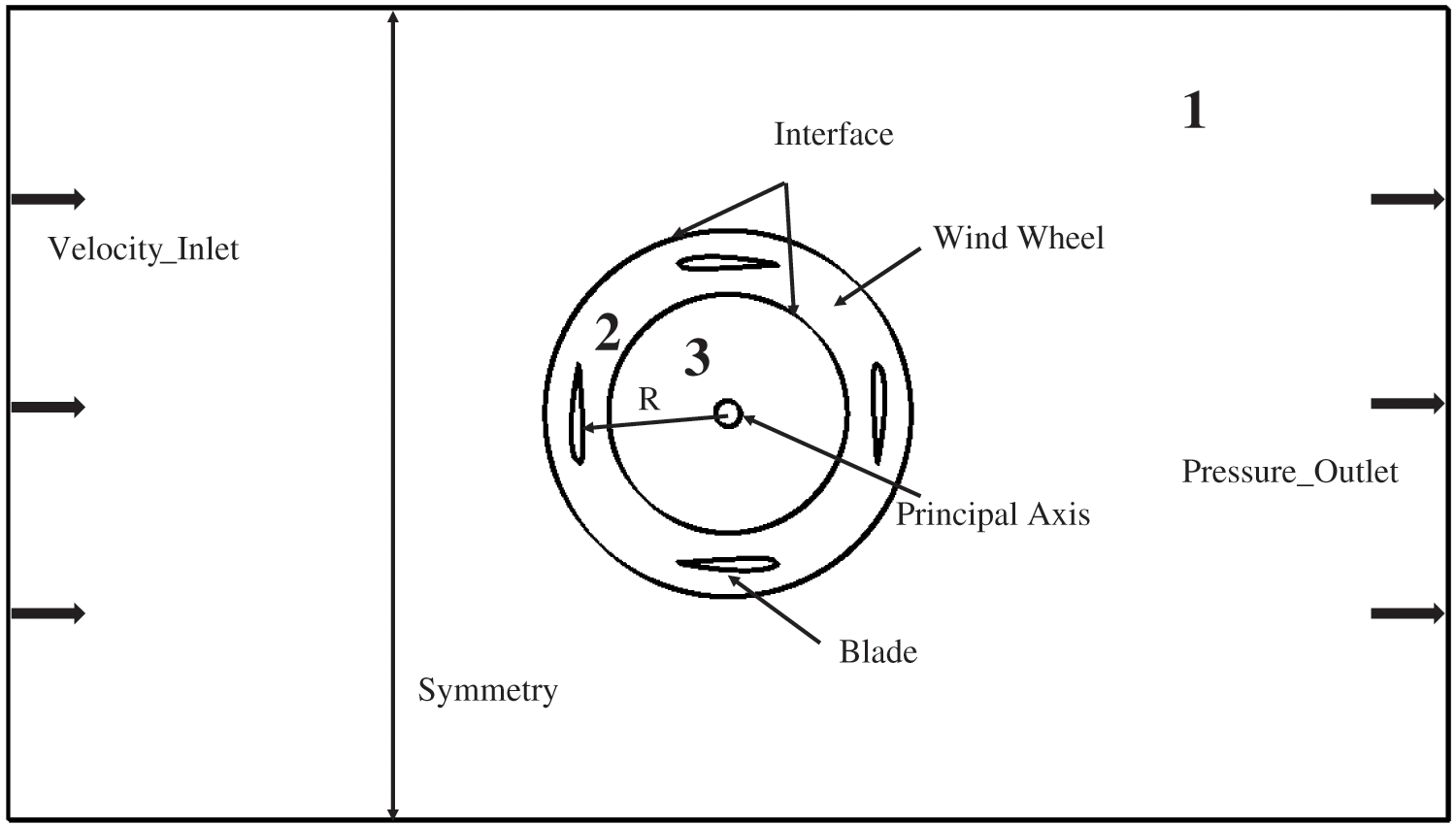
Figure 6: Calculation domain and boundary conditions of the vertical axis wind turbine

In this paper, unstructured meshing is used, and to improve the quality of the airfoil mesh, the boundary layer command is used to mesh the boundary layer of the airfoil. The mesh growth rate is 1.05, and the number of layers is 10 layers. The wind wheel mesh is encrypted to minimize the error of the simulation results. The meshing of the H-type vertical axis wind turbine calculation domain is shown in Fig. 7, and the entire calculation domain includes 645247 grids and 419865 nodes. Among them, Fig. 7a is the rotation domain mesh, Fig. 7b is the airfoil perimeter mesh, the airfoil perimeter mesh is encrypted, and Fig. 7c is the grid of the entire computing domain.

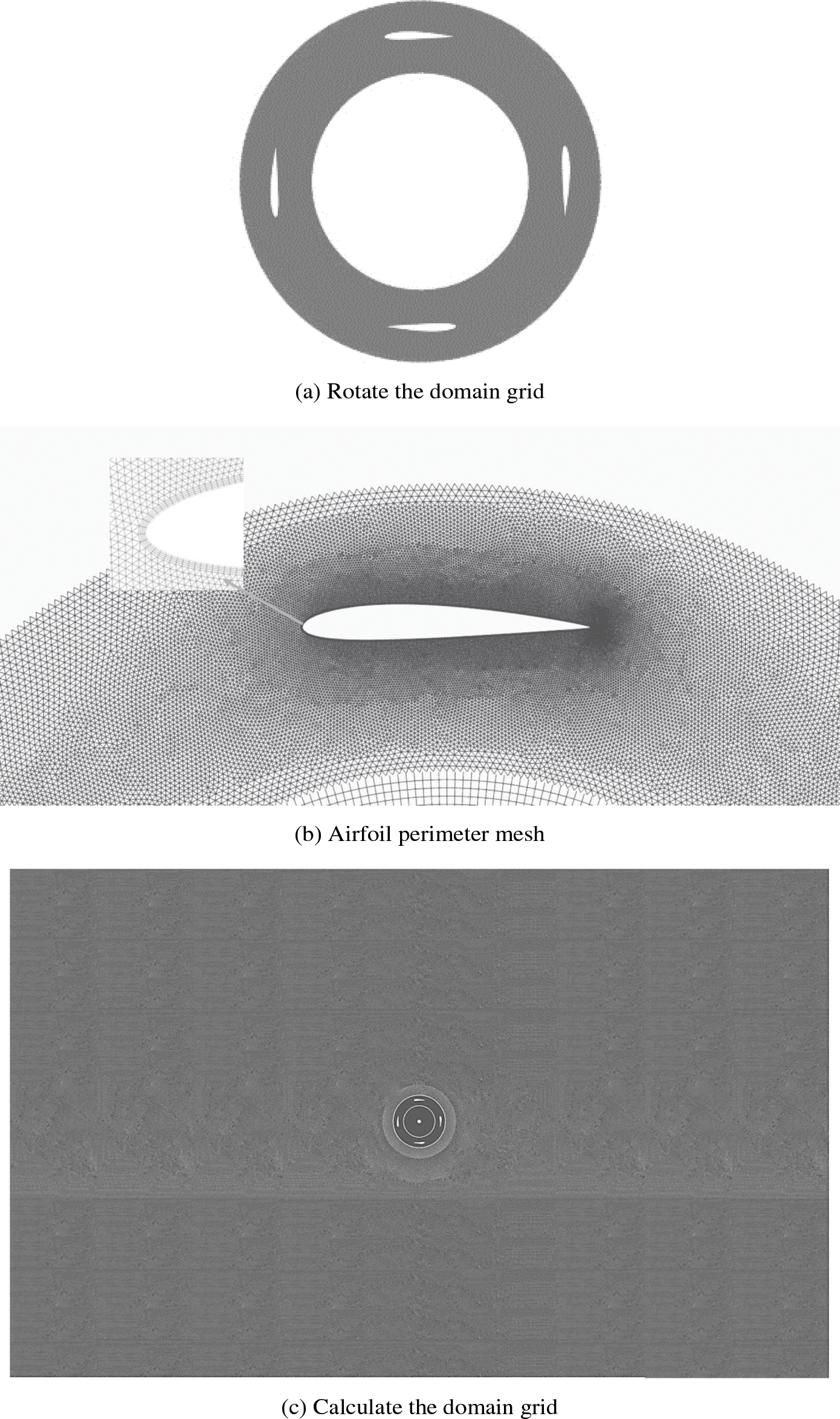
Figure 7: Wind turbine computing domain grid

4.3 Turbulence Model Selection and Solver Settings

The external flow field of the vertical axis wind turbine is an unsteady flow, and the rotation of the wind wheel produces strong disturbance, so it is more reasonable to choose the Renormalization Group (RNG) model [14]. Therefore, the RNG k-ε model was selected as the turbulence model, and the pressure solver was selected. Using the SIMPLE algorithm, the discrete format is second-order windward [15].

4.4 Irrelevance Verification

4.4.1 Grid Independence Verification

In this paper, four sets of computational domain grids with different densities are set, and the number of grids are 398745, 509476, 605247, and 718544, respectively. In the incoming flow, the wind speed is v = 10 m/s, and the tip speed ratio is λ = 1.95. Under the working environment, the numerical simulation calculation is carried out for the H-type vertical axis wind turbines with different grid numbers in each group, and the calculation results are shown in Table 3.

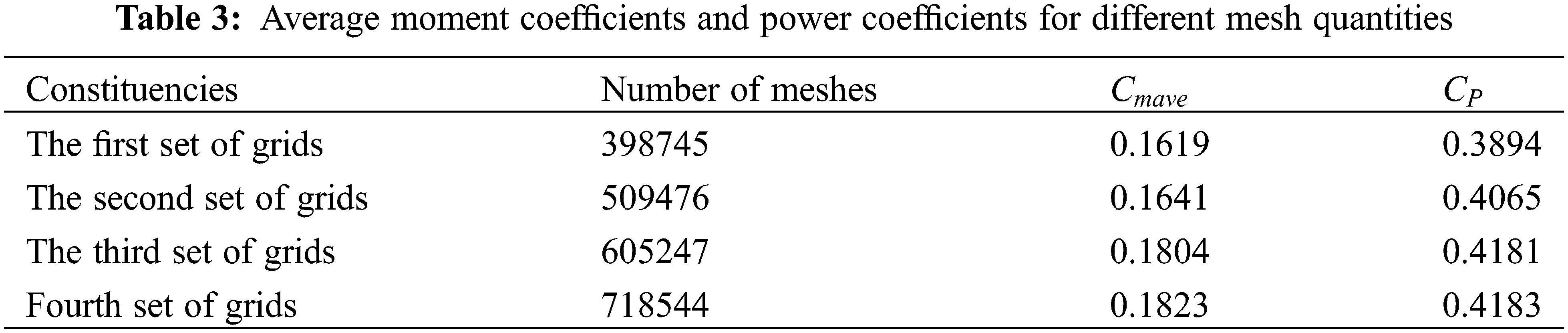
Fig. 8 shows the average moment coefficient curve for different mesh numbers. The average moment coefficient of the first set of grids is different from the second set of meshes by 1.4%. The average torque coefficient of the second group of grids is quite different from that of the third group. The average moment coefficient of the third group of grids differs by less than 1% from the fourth group. After the number of meshes reaches 600,000, the average moment coefficient curve tends to be smoothed. From the third set of mesh instructions, the improvement in the accuracy of the grid and numerical simulation calculation is very small, because the number of meshes is too large, which will greatly increase the time cost.

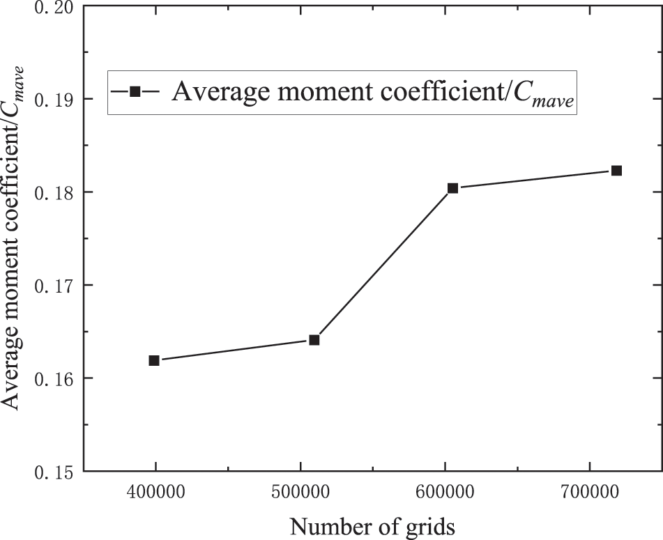
Figure 8: Average moment coefficient curve for different mesh quantities

Fig. 9 shows the power coefficient curve under different mesh numbers. The power coefficient gradually increases as the number of grids increases, and after the number of grids reaches 600,000, the power coefficient increases slightly as the number of grids increases. In summary, to better save time and cost, the third set of grids is selected to complete the subsequent numerical simulation calculation.

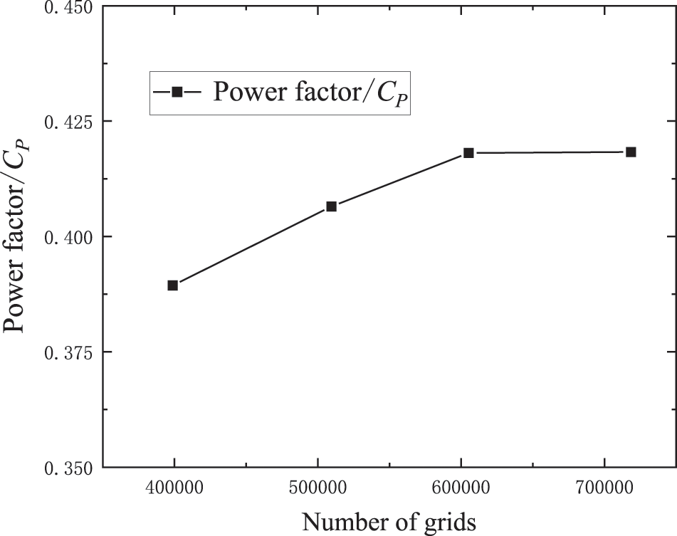
Figure 9: Power coefficient curves under different mesh numbers

4.4.2 Time Independence Verification

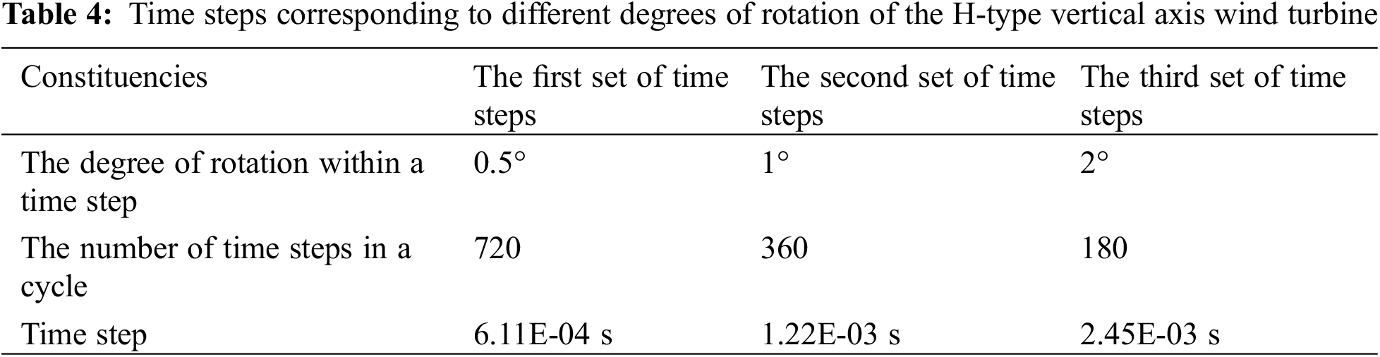
To avoid the influence of time step on the accuracy of the numerical simulation results of the H-type vertical axis wind turbine, three different sets of time steps are set in this paper, which are the corresponding time steps of 0.5°, 1° and 2° rotation of the vertical axis wind turbine, as shown in Table 4.

From the three different sets of time steps set in Table 4, the moment coefficient curve of the single blade of the H-type vertical axis wind turbine is obtained as shown in Fig. 10.

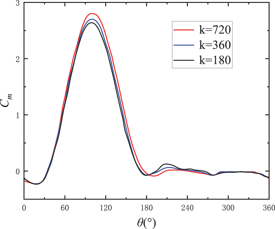
Figure 10: Moment coefficient curve of a single blade at different time steps

In the rotation cycle, the numerical simulation results of different short periods of time are set, and the moment coefficient curves of a single blade of the H-type vertical axis wind turbine almost coincide, and the change trend is consistent. The force distance coefficient curves corresponding to the rotation degrees of 1° and 2° in the set time step are almost the same, with only a slight deviation at the peaks of the curves. The moment coefficient curve with a rotation degree of 0.5° and the torque coefficient curve of 1° and 2° in the set time step are significantly larger at the peak of the curve. The numerical simulation calculation time cost of setting the rotation degree in the time step is 0.5°, so the time step corresponding to the rotation of 1° in the time step is selected as the most suitable time step under the premise that the numerical simulation calculation accuracy can be guaranteed.

4.5 Analysis of Calculation Results

4.5.1 Power Coefficient and Torque Coefficient

The number of rotation cycles of the vertical axis wind turbine obtained from the numerical simulation has a significant impact on the accuracy and stability of the calculation results. According to the research of Jia et al. [16], the data of 15 rotation cycles of the wind turbine is selected for analysis. The moment coefficient CT and power coefficient CP (wind energy utilization ratio) of the vertical axis wind turbine are important parameters to measure the performance of the wind turbine. The calculation formula is:

CT=T(0.5ρV2AR) (22)

CP=P(0.5ρV3A)  (23)

where: CP is the power factor (i.e., the rate of utilization of wind energy); CT is the moment coefficient; R is the radius of wind turbine (m); V is the incoming wind speed (m/s); T is the resultant moment of four blades; ρ is the air density (kg/m3); A is the windward area of the wind turbine (m2).

According to the calculation formula of the power coefficient of the vertical axis wind turbine, the power coefficient is directly proportional to its tip speed ratio, and its power coefficient increases with the increase of the tip speed ratio. Fig. 11 shows the power curve comparison between the optimized airfoil and the original airfoil. At the same tip speed ratio, the power coefficient of the optimized airfoil is significantly improved, and when the tip speed ratio is 1.95, the maximum power coefficient of the wind turbine is 0.453, which is 12.19% higher than the original airfoil.

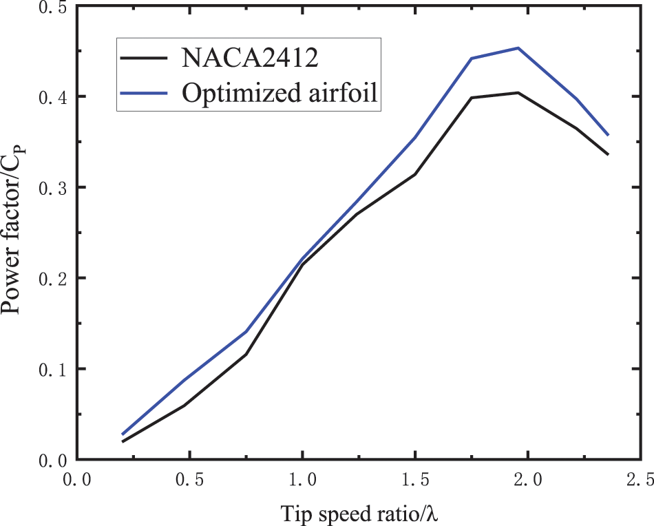
Figure 11: Comparison of the average power coefficient curves of the optimized airfoil and the original airfoil

The torque coefficient CT of the vertical axis wind turbine can perfectly express the torque borne by the wind turbine during normal operation. Therefore, in the process of FLUENT software simulation calculation of the wind turbine, its torque coefficient can be used as the detection object to monitor and control the operation of the wind turbine rotor in real time. Fig. 12 shows the torque coefficient curve of the vertical axis wind turbine operating in 360° range. The torque coefficient of the optimized blade has been significantly improved compared with the original blade in the rotation cycle of the vertical axis wind turbine, which greatly improves the wind energy conversion capacity of the wind turbine.

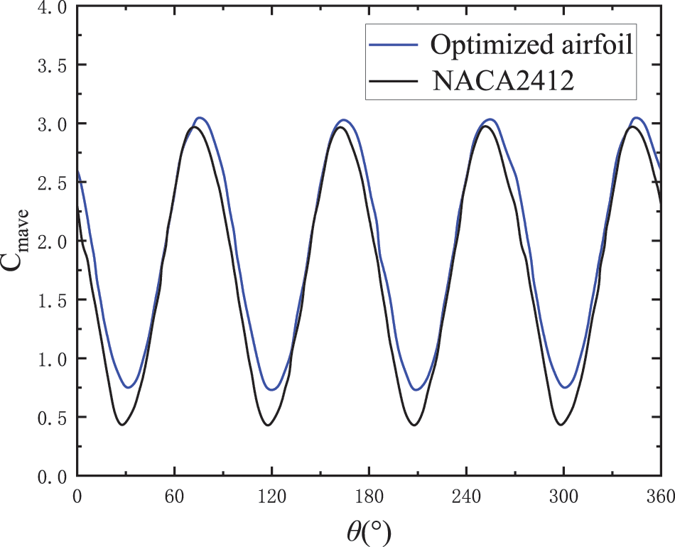
Figure 12: Comparison of the four-blade combined moment coefficient curves of the vertical axis wind turbine ( λ=1.95 )

4.5.2 H-Type Vertical Axis Wind Turbine Speed Distribution

In this paper, the CFD flow field simulation of the H-type vertical axis wind turbine is verified under the condition that the blade tip speed ratio is λ = 1.95. Fig. 13 shows the velocity distribution of the H-type vertical axis wind turbines before and after airfoil optimization at different rotation angles.

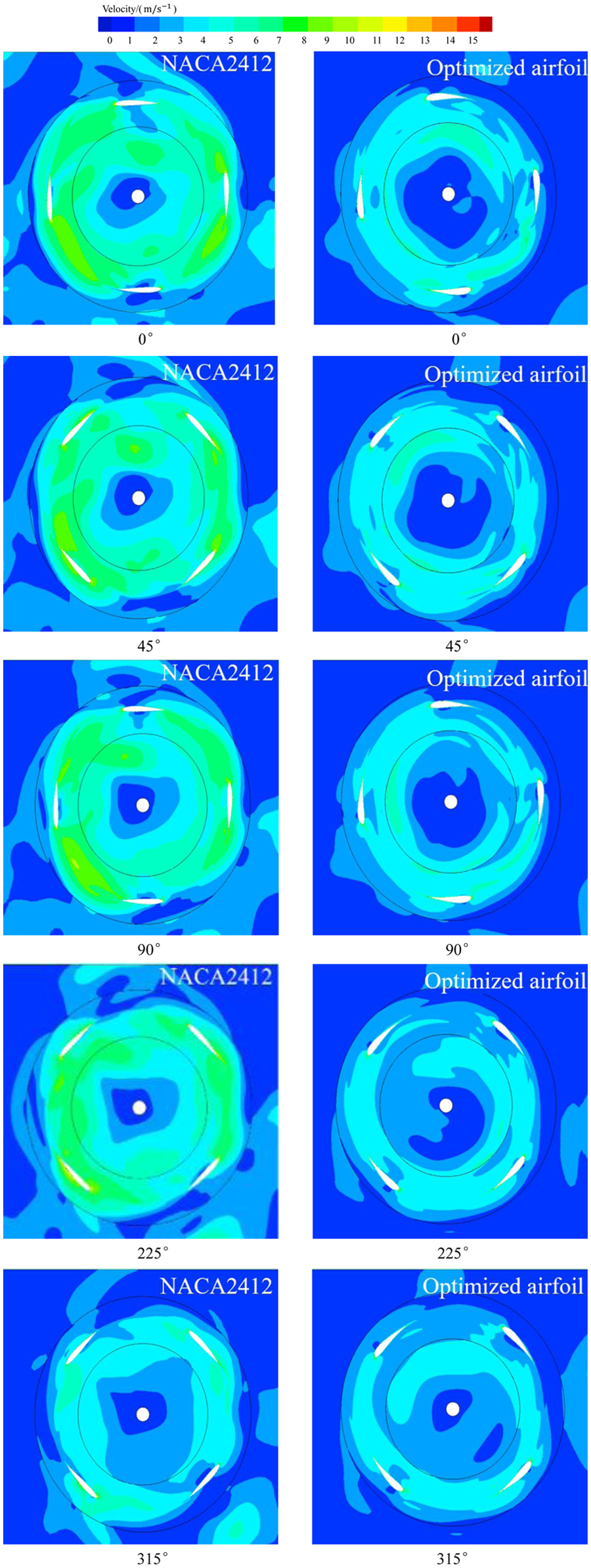
Figure 13: Velocity distribution of the original and optimized airfoils

When the rotation angle of the wind turbine is 0°, the air flow velocity in the domain field is split at the leading edge and trailing edge of the airfoil, and the air flow velocity at the leading edge and trailing edge of the airfoil increases significantly. When the rotation angle of the wind turbine starts from 45°, the gas flow split point gradually moves down along the leading edge of the airfoil curve, and the gas flow rates at the leading edge and trailing edge of the airfoil gradually increase. When the rotation angle is 225°, the leading-edge speed gradually decreases. When the rotation angle of the wind turbine is 315°, vortexes appear on the upper wing surface of the blades, and the vortexes that appear on the optimized blade are obviously smaller than those on the original blade. The appearance of these vortexes will cause the wind turbine blade to stall, which can lead to blade damage. The optimized blade will also stall, but compared with the original blade, the optimized blade can effectively restrain the stall phenomenon of the blade, thus greatly improving the aerodynamic performance of the blade and enhancing the safety factor of the wind turbine.

4.5.3 H-Type Vertical Axis Wind Turbine Pressure Distribution

Fig. 14 shows the pressure distribution of the H-type vertical axis wind turbine at different rotation angles before and after optimization of the airfoil.

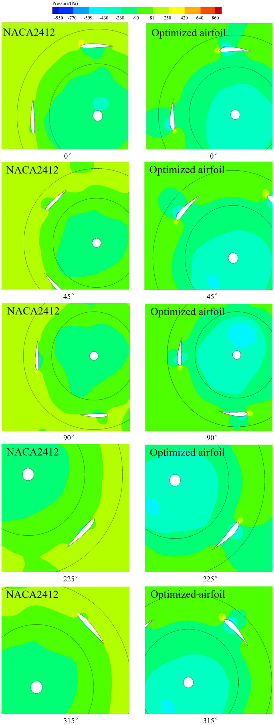
Figure 14: Pressure distribution of the original and optimized airfoils

When the rotation angle of the wind turbine is 0°, the external pressures on the upper and lower surface contours of the original airfoil and the optimized airfoil are symmetrically distributed, and the maximum pressures are located above the leading edge of the airfoil. When the wind turbine rotates to 90°, the external pressure distribution on the upper and lower surfaces of the original airfoil gradually becomes irregular. The maximum pressure of the optimized airfoil is always at the leading edge of the airfoil, and it gradually moves down along the leading edge of the airfoil with the increase of the rotation angle. In this process, the pressure difference between the upper and lower surface contours of the optimized airfoil and the original airfoil increases continuously, and the growth rate of the pressure difference between the upper and lower surface contours of the optimized airfoil is higher than that of the original airfoil. With the increase of the wind turbine rotation angle to 315°, the pressure acting on the surface of the original airfoil and the optimized airfoil changes from the upper to the lower surface. The pressure difference at any rotation angle of the wind turbine acts on the wind turbine as the same rotational force, and the pressure difference between the upper and lower wing surfaces at any rotation angle of the optimized airfoil wind turbine is higher than that of the original airfoil wind turbine.

4.5.4 Distribution of Blade Pressure Coefficient of the H-Type Vertical Axis Wind Turbine

Fig. 15 shows the pressure coefficient distribution diagram of the H-type vertical axis wind turbine blades before and after optimization at different azimuth angles.

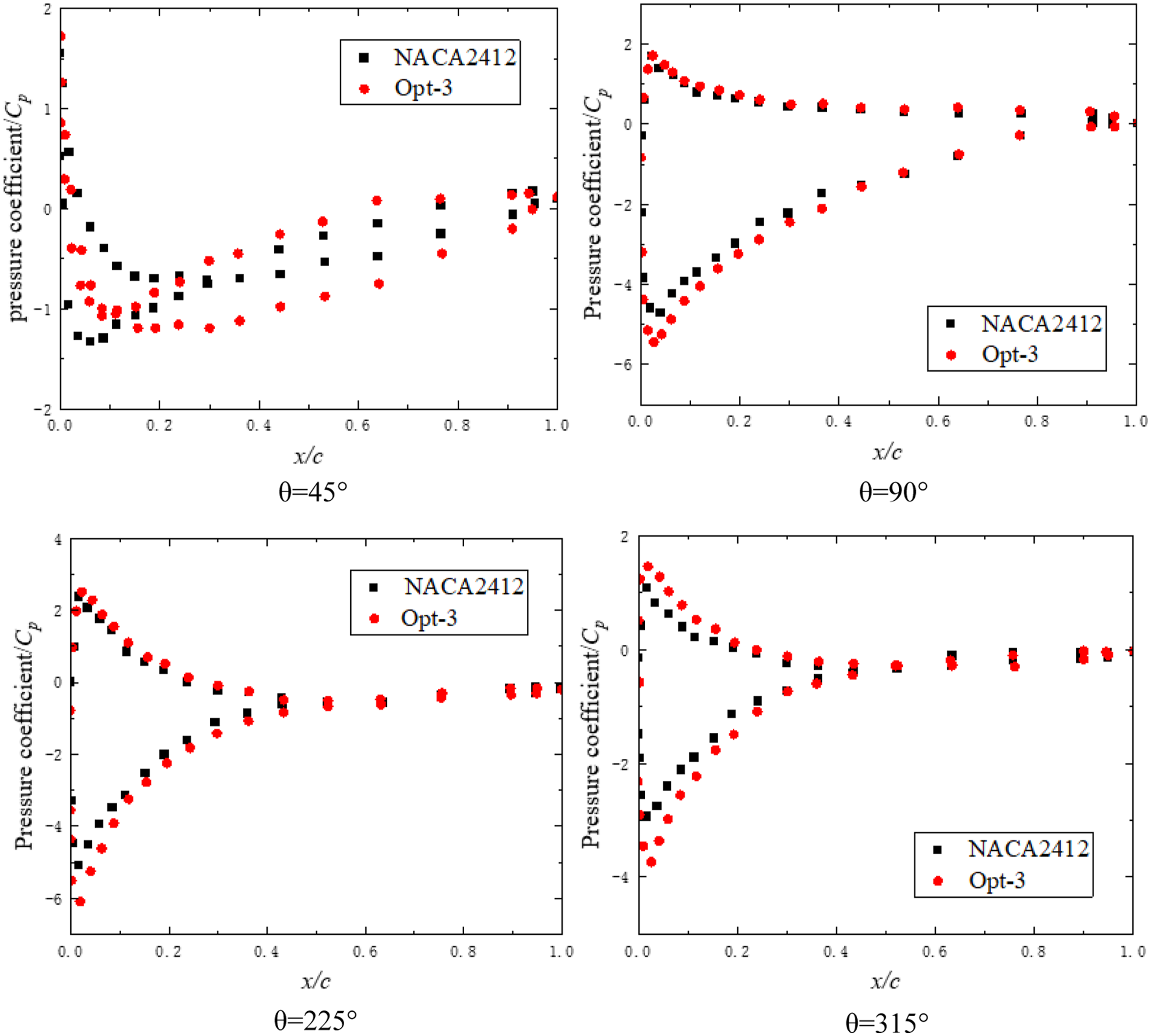
Figure 15: Pressure coefficient distribution of the H-type vertical axis wind turbine blades at different azimuth angles ( λ= 1.95)

The absolute value of the optimized blade pressure coefficient of the wind turbine is slightly larger than that of the original blade under different azimuth angles; In the range of 0 < x/c < 0.45, the pressure coefficient difference on the blade surface is large; In the range of 0.45 < x/c < 1, the pressure coefficient difference on the blade surface does not change significantly. This shows that flow separation occurs at the inner side of the leading edge of the blade at the trailing edge of the blade.

5  Conclusion

(1) In this paper, the Bézier curve is used to fit the airfoil curve, and its aerodynamic performance is characterized. The maximum thickness, maximum bending position, and maximum bending of the airfoil are taken as its constraint variables, which provides the requirements for completeness or the optimization design of the original airfoil NACA 2412 and provides a theoretical reference for the optimization design of the airfoil.

(2) The lift coefficient and lift drag ratio of the optimized airfoil are significantly higher than those of the original airfoil, and the stall performance of the optimized airfoil is improved. The maximum lift coefficient of the optimized airfoil is 8.33% higher than that of the original airfoil. The maximum lift drag ratio of the optimized airfoil is 11.22% higher than that of the original airfoil. During the rotation period, the power coefficient of the vertical axis wind turbine equipped with optimized blades exceeds 12.19% compared with the original blades.

Funding Statement: This study was supported by the following research funding. Natural Science Foundation of Anhui Province, China, Grant Number 1908085ME166. Research on the Key Technology of Multipole Grain Sampling and Inspection Equipment Based on Machine Vision, Anhui Provincial Grain Machinery Rural Development Collaborative Technology Service Center, Grant Number GXXT-2022-077. Research on the Preparation Process and Application of Biochar Made of Bamboo, Science and Technology Bureau of Chuzhou City, Grant Number 2022ZN014. The Development and Industrialization of Fruit Sorting Equipment, Science and Technology Bureau of Chuzhou City, Grant Number 2022ZN016. Natural Science Major Project of Anhui Provincial Education Department, Anhui Provincial Education Department, Grant Number 2022AH040238. Key Scientific Research Project of Anhui Provincial Education Department, Anhui Provincial Education Department, Grant Number KJ2021A0877.

Conflicts of Interest: The authors declare that they have no conflicts of interest to report regarding the present study.

References

1. Liu, X. L., Chen, Q., Yang, B., Song, M. R. (2020). Research on the performance of a vertical-axis wind turbine with helical blades by detached eddy simulation. Journal of Solar Energy Engineering, 142(3), 031008. [Google Scholar]

2. Bajhdadi, M., Elkoush, S., Akle, B., Elkhoury, M. (2020). Dynamic shape optimization of a vertical-axis wind turbine via blade morphing technique. Renewable Energy, 154(9), 239–251. [Google Scholar]

3. Li, Y. J., Wei, K. X., Yang, W. X., Wang, Q. (2020). Improving wind turbine blade based on multi-objective particle swarm optimization. Renewable Energy, 161(3), 525–542. [Google Scholar]

4. Ma, Y., Zhang, A., Yang, L. (2019). Investigation on optimization design of offshore wind turbine blades based on particle swarm optimization. Energies, 12(10), 1–218. [Google Scholar]

5. Zhang, J., Shi, K., Liao, C. (2018). Improved particle swarm optimization of designing resonance fatigue tests for large-scale wind turbine blades. Journal of Renewable and Sustainable Energy, 10(5), 053303. [Google Scholar]

6. Rezaeiha, A., Kalkman, I., Blocken, B. (2017). Effect of pitch angle on power performance and aerodynamics of a vertical axis wind turbine. Applied Energy, 197(8), 132–150. [Google Scholar]

7. Amine, B., José, C. P. (2023). Enhancement of a cycloidal self-pitch vertical axis wind turbine performance through DBD plasma actuators at low tip speed ratio. International Journal of Thermofluids, 17(8), 100258. [Google Scholar]

8. Song, C. G., Wu, G. Q., Zhu, W. N., Zhang, X. D. (2020). Study on aerodynamic characteristics of darrieus vertical axis wind turbines with different airfoil maximum thicknesses through computational fluid dynamics. Arabian Journal for Science and Engineering, 45(2), 689–698. [Google Scholar]

9. Celik, Y., Ma, L., Derek Ingham, D., Pourkashanian, M. (2020). Aerodynamic investigation of the start-up process of H-type vertical axis wind turbines using CFD. Journal of Wind Engineering & Industrial Aerodynamics, 204, 104252. [Google Scholar]

10. Zhang, Z. Y., Chen, M., Zhang, X., Wang, Z. P. (2008). Analysis of inflection points for planar cubic bezier curve. Journal of Symbolic Computation, 43, 92–117. [Google Scholar]

11. Hu, X. Y., Li, Z. H., Bao, R. H., Chen, W. Q. (2022). An adaptive method of moving asymptotes for topology optimization based on the trust region. Computer Methods in Applied Mechanics and Engineering, 393, 114202. [Google Scholar]

12. Robert, A. L. M., Marius, P. (2020). Simulation based analysis of morphing blades applied to a vertical axis wind turbine. Energy, 202(11), 117705. [Google Scholar]

13. McLaren, K. W. (2011). A numerical and experimental study of unsteady loading of high solidity vertical axis wind turbines. Mc Master University, Hamilton. [Google Scholar]

14. Ismail, M. F., Vijayaraghavan, K. (2015). The effects of aerofoil profile modification on a vertical axis wind turbine performance. Energy, 80(1), 20–31. [Google Scholar]

15. Maalouly, M., Souaiby, M., Elcheikh, A., Issa, J. S. (2022). Transient analysis of H-type vertical axis wind turbines using CFD. Energy Reports, 8, 4570–4588. [Google Scholar]

16. Jia, R. Y., Xia, H. J., Zhang, S., Su, W. G., Xu, S. H. (2022). Optimal design of Savonius wind turbine blade based on support vector regression surrogate model and modified flower pollination algorithm. Energy Conversion and Management, 270(5), 116–247. [Google Scholar]