Numerical Analysis of the Influence of Turbulence Intensity on Iced Conductors Gallop Phenomena

1  Introduction

The cross-section shape of the conductor will change after an overhead transmission conductor is iced, that is, from a circular section to a non-circular section. The lift, drag, and torque of an iced conductor with a non-circular cross-section under wind load can easily induce galloping [1]. The basic characteristic of iced conductor galloping is low frequency and large amplitude. The frequency range of iced conductor galloping is approximately 0.1–3 Hz, and the amplitude range is approximately 5–300 times of the wire diameter. When the iced conductor galloping occurs, the large galloping amplitude can easily cause line tripping, metal wear, power failure, broken insulator string, tower arm damage and other accidents [2]. Therefore, the research on transmission line galloping is the key research direction in the fields of electrical and material engineering.

Given the phenomenon of galloping iced conductors, researchers have conducted in-depth research on the galloping mechanism and put forward various corresponding measures to prevent galloping. In the study of the galloping mechanism of iced conductors, the transverse galloping, torsional galloping, and eccentric inertial coupling mechanisms [3–6] have been widely recognized by the academic community. Luongo et al. [7] established the galloping model of an iced single conductor using a beam element. In addition, based on the experimental results, Keutgen et al. [8] used the numerical simulation method to study the galloping phenomenon of iced conductors to verify the rationality of the numerical method. Meanwhile, Sansica et al. [9] deduced the dynamic equation in the time series of lift coefficient by the SINDy algorithm and completed the modeling of the Stuart-Landau oscillator, which reduced the calculation time from hundreds of core hours to seconds. Diana et al. [10] used the finite element method and quasi-steady state theory to simulate the system structure and reproduce the fluid elastic force to realize galloping simulation and verified it with real cases. Thus, time domain simulation and energy method were used in this process, which had good results from the engineering point of view.

However, transmission conductors are in a complex turbulent environment in practical engineering. Wind tunnel tests that study the galloping characteristics of iced conductors are generally carried out in wind tunnels with low turbulence intensity. Therefore, it is necessary to consider the influence of turbulence intensity in the study of transmission conductor galloping. Yan et al. [11] carried out wind tunnel tests on an iced conductor with different shapes and obtained the aerodynamic coefficients of the iced conductor under different turbulence intensities. Moreover, Chadha et al. [12] adopted similar test methods for conductor with non-symmetric shape, and measured the aerodynamic coefficients of the model under uniform flow fields, 7%, and 18% turbulence flow fields, however, they did not conduct experimental analysis on the split conductor. Renaud et al. [13] obtained the aerodynamic coefficients of ice-covered conductors with non-symmetric shape cross-sections with uniform flow and 18% uniform turbulence in the wind tunnel laboratory using the force balance. Japanese researcher Shimizu et al. [14] studied the aerodynamic characteristics of the conductor with non-symmetric shape section under uniform flow through wind tunnel tests. Meanwhile, Istvan et al. [15] studied the law of the influence of turbulence on the internal structure of an airfoil separation bubble by wind tunnel test with Re = 8 × 104. The mentioned researchers primarily studied the aerodynamic characteristics of iced conductors, while there are few analyses on the galloping response of iced conductors under different turbulence intensities. However, most studies are based on the quasi-steady-state assumption model, and the mutual coupling between the iced conductor and the flow field is not considered. Given that the iced conductor is excited by the wind, different kinds of vibration will occur, and the vibration of the conductor will react to the flow field to form a complex fluid-solid coupling vibration. Therefore, it is necessary to use the fluid-solid coupling method to analyze the galloping of iced conductors under different turbulence intensities.

Consequently, the galloping response of a conductor with a non-symmetric shape under different turbulence intensities (5%, 15%, and 25%) is studied by the fluid-solid coupling method. The user-defined function (UDF) is written to solve the motion control equation of the iced conductor, and the real-time displacement of the iced conductor in the flow field is obtained through the secondary development of Fluent finite element software. Combined with the nested grid technology, the flow field grid is updated to realize the fluid-solid coupling calculation. Furthermore, the variation of the aerodynamic coefficient of the iced conductor with the angle of attack under different turbulence intensities is compared and analyzed, as well as the variation of the galloping amplitude of the iced conductor under different turbulence intensities and different wind speeds at the same angle of attack. Hence, it can provide a theoretical reference for the in-depth study of the galloping mechanism and anti-galloping technology of iced conductors.

2  Governing Equation

Fluid continuity and N-S equations are as follows [16]:

Continuity equation

∂u∂x+∂ν∂y=0 (1)

Momentum equation

{∂u∂t+u∂u∂x+v∂u∂y=μρ(∂2u∂x2+∂2u∂y2)−1ρ∂p∂x∂v∂t+u∂u∂x+v∂u∂y=μρ(∂2v∂x2+∂2v∂y2)−1ρ∂p∂y (2)

where u and v are the velocities (m/s) of the fluid in the x and y directions, respectively; μ is the dynamic viscosity coefficient (m2/s); ρ is fluid density (kg/m3); and p is the fluid pressure (N/m2).

The expression of the momentum equation after Reynolds averaging is as follows:

∂∂t(ui)¯+∂∂xj(ui¯uj¯)=−1ρ∂p¯∂xi+∂∂xj(μρ∂ui¯∂xj−u′iu′j¯), (i=1, 2, 3) (3)

For incompressible fluids, the expression of turbulent stress term is as follows:

−ρu′iu′j¯=μt(∂ui¯∂xj+∂uj¯∂xi)−23(ρk+μt∂ui∂xi)δij (4)

where μt is the turbulent viscosity; δij is the “Kronecker Delta” symbol, when i = j = 1, then δij = 1, when i ≠ j, then δij = 0.

k is the turbulent kinetic energy:

k=u′iu′j¯/2=(u′12¯+u′22¯+u′32¯)/2 (5)

The SST k-ω model determines turbulent viscosity (turbulence kinetic energy equation and turbulent diffusion equation) through two differential equations, and its equation expression is as follows:

{∂(ρk)∂t+∂(ρku)∂x=∂∂y(Γk∂k∂y)+Gk−Yk∂(ρω)∂t+∂(ρωu)∂x=∂∂y(Γω∂ω∂y)+Gω−Yω+Dω (6)

where Gk is the turbulent kinetic energy generation term; Gω is the production term of turbulent dissipation rate ω; Γk and Γω are the effective diffusion coefficients of turbulent kinetic energy k and turbulent dissipation rate ω, respectively; and Yk and Yω are the turbulent kinetic energy k and turbulent dissipation rate ω based on turbulent dissipation term, respectively. Dω is the cross-diffusion coefficient.

The effective diffusion term [17] is defined by the SST k-ω turbulence model Γk and Γω.

Γk=μ+μtσk (7)

Γω=μ+μtσω (8)

where σk and σω are turbulent Prandtl number about k and ω; and μt is the turbulent viscosity coefficient [17], which can be obtained by the following formula:

μt=ρkω⋅1max(1a∗, SF2a1ω)(9)

where s is the strain rate; and a1 is the model parameter and a1 = 0.31. σk and σω are defined as follows:

σk=1F1/σk,1+(1−F1)/σk,2 (10)

σω=1F1/σω,1+(1−F1)/σω,2 (11)

where F1 and F2 are mixed functions. The definition of a* in the turbulent viscosity coefficient μt [17] is as follows:

a∗=a∞∗(a0+Re1/Rk1+Re1/Rk) (12)

where Re1 = ρk/μω; Rk = 6; a0 = βi/3, βi = 0.072; generally, for the SST k-ω two-equation turbulence model with a high Reynolds number, a* = a∞* = 1.

The pressure distribution on the surface of the positive feeder can be obtained by calculating the flow field, and then the lift FL and drag FD acting on the positive feeder can also be obtained.

The aerodynamic loads on the surface of the iced conductor are expressed as follows [18]:

FD=12ρU2LDCDFL=12ρU2LDCLFM=12ρU2LD2CM (13)

The calculation model of conductor vibration can be simplified as a quality-stiffness-damping system. By defining m, k and c as the quality, spring stiffness, and damping of the system, respectively, the vibration equation of the three-degree-of-freedom model can be expressed as follows [19]:

mx¨+2mζx0ωx0x˙+mωx02x=FDmy¨+2mζy0ωy0y˙+mωy02y=FLIθ¨+2Iζθ0ωθ0θ˙+Iωθ02θ=FM (14)

In the formula: x and y are the horizontal and vertical displacements respectively; θ is the torsion angle caused by the change of the overall shape center of the conductor after icing; ζx0, ζy0, and ζθ0 are the damping ratios in horizontal, vertical, and torsional directions, respectively; ωx0, ωy0 and ωθ0 are the angular frequencies in the horizontal, vertical, and torsional directions, respectively, which are 2π times of the natural frequency; and I is the inertial mass moment per unit length of the iced conductor.

Combined with Eq. (13), the motion control equation of the iced conductor can be obtained. The displacement, velocity, and acceleration of the conductor motion can be obtained by solving the iced conductor’s motion control equation.

mx¨+2mζx0ωx0x˙+mωx02x=ρU2LDCD2my¨+2mζy0ωy0y˙+mωy02y=ρU2LDCL2Iθ¨+2Iζθ0ωθ0θ˙+Iωθ02θ=ρU2LD2CM2 (15)

2.1 Analysis of Galloping Stability

Based on the Den Hartog vertical galloping mechanism, the stability of the iced conductor can be judged by the following formula [20]:

Den=∂CL∂α+CD<0 (16)

Den is the Den Hartog coefficient.

Meanwhile, based on the Nigol galloping mechanism, the torsional vibration is self-excited vibration when the icing satisfies certain conditions. The critical condition for the torsional instability of conductors can be expressed as follows:

Nigol=∂CM∂α (17)

In the formula, when the Nigol coefficient ∂CM/∂α <0, the iced conductor may be galloping. The Den Hartog coefficient and the Nigol coefficient of iced conductors under different turbulence intensities can be obtained by derivation of the lift coefficient and torsion coefficients.

3  Calculation Model and Parameter Setting

3.1 Calculation Model and Mesh Division

The 2D rectangular flow field is used as the calculation area of the whole flow field. The centroid of the conductor coincides with the origin of the initial coordinate. The horizontal direction is downstream, whereas the vertical direction is crossflow. The length of the upstream inflow area in the fluid calculation domain is 3 m, and the length of the downstream wake area is 4 m to ensure the full development of the conductor wake. In addition, the upper and lower boundaries are set at 2 m to meet the requirements of the blocking rate and dynamic mesh. The flow field calculation model is shown in Fig. 1. Moreover, the grid height of the first layer of the boundary layer is 1 × 10−4, and the normal growth rate is 1.1 to ensure y+ < 1. When calculating in Fluent, the spanwise length of the 2D model is 1 m by default. In this paper, the Reynolds number is in the subcritical range of a high Reynolds number, and the SST k-ω is the turbulence model. The boundary conditions are set as follows: the pressure-based algorithm is used to solve the 2D steady incompressible N-S equation, the Coupled method is used for pressure-velocity coupling, and the second-order upwind scheme of the Green-Gauss formula is selected to discretize the equation. The entrance boundary of the calculation domain is set as the velocity entrance, the velocity is 15 m/s, and the direction is determined by the attack angle of the incoming flow. Moreover, the exit boundary is set as the pressure exit, the pressure is 0 Pa, the conductor surface is the boundary of a non-slip solid wall, and the convergence residual is less than 1 × 10−6.

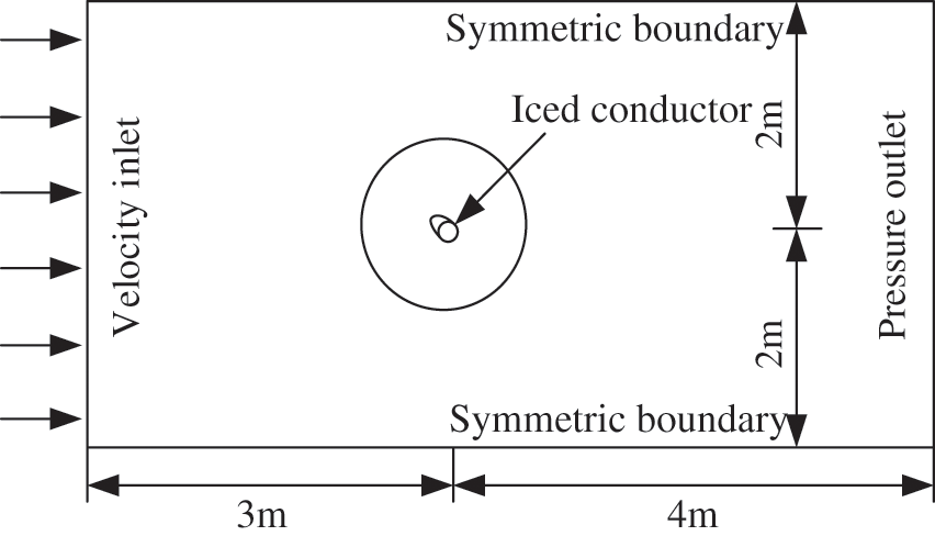
Figure 1: Calculation model

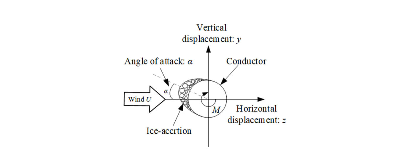
The wind attack angle α is the relative angle between the incoming airflow and the model. In aerodynamics, the 0° or 180° direction of the incoming airflow attack angle is generally set as the direction parallel to the symmetry axis of the model section, The model is positive when it rotates clockwise and negative when it rotates counterclockwise. Directions of aerodynamic forces and wind angle are shown in Fig. 2.

Figure 2: Directions of aerodynamic forces and wind angle

Fig. 3 is the stress analysis diagram of the iced conductor, where Fy and Fz are the aerodynamic forces in vertical and horizontal directions, respectively. By analyzing the force of the conductor, these forces are obtained as follows:

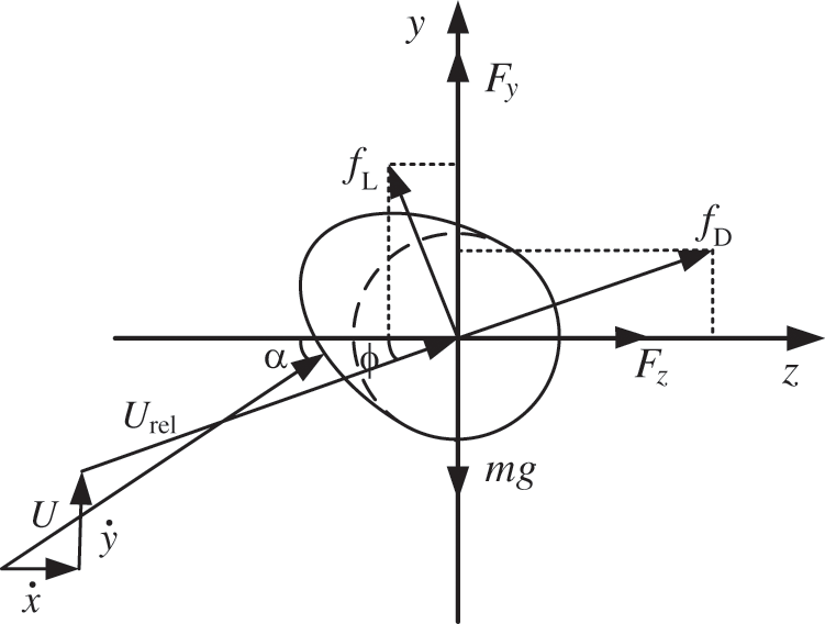
Figure 3: Force analysis diagram of the iced conductor

In Fig. 3, the iced conductor vibrates in x and y directions under the action of uniform incoming flow U. The vibration velocity is x and y, α is the relative wind attack angle, which indicates the angle formed by the incoming flow and the front vertical line of the iced conductor. Meanwhile, φ is the relative wind attack angle, which indicates the angle formed by the resultant force direction formed by the real incoming flow direction and the conductor movement direction when the iced conductor is galloping. Urel is the relative wind speed between the incoming wind and the conductor, fL and fD are the lift and drag of the iced conductor under the action of relative wind speed, and FZ and Fy are the horizontal and vertical forces of the iced conductor under the rectangular coordinate system, respectively.

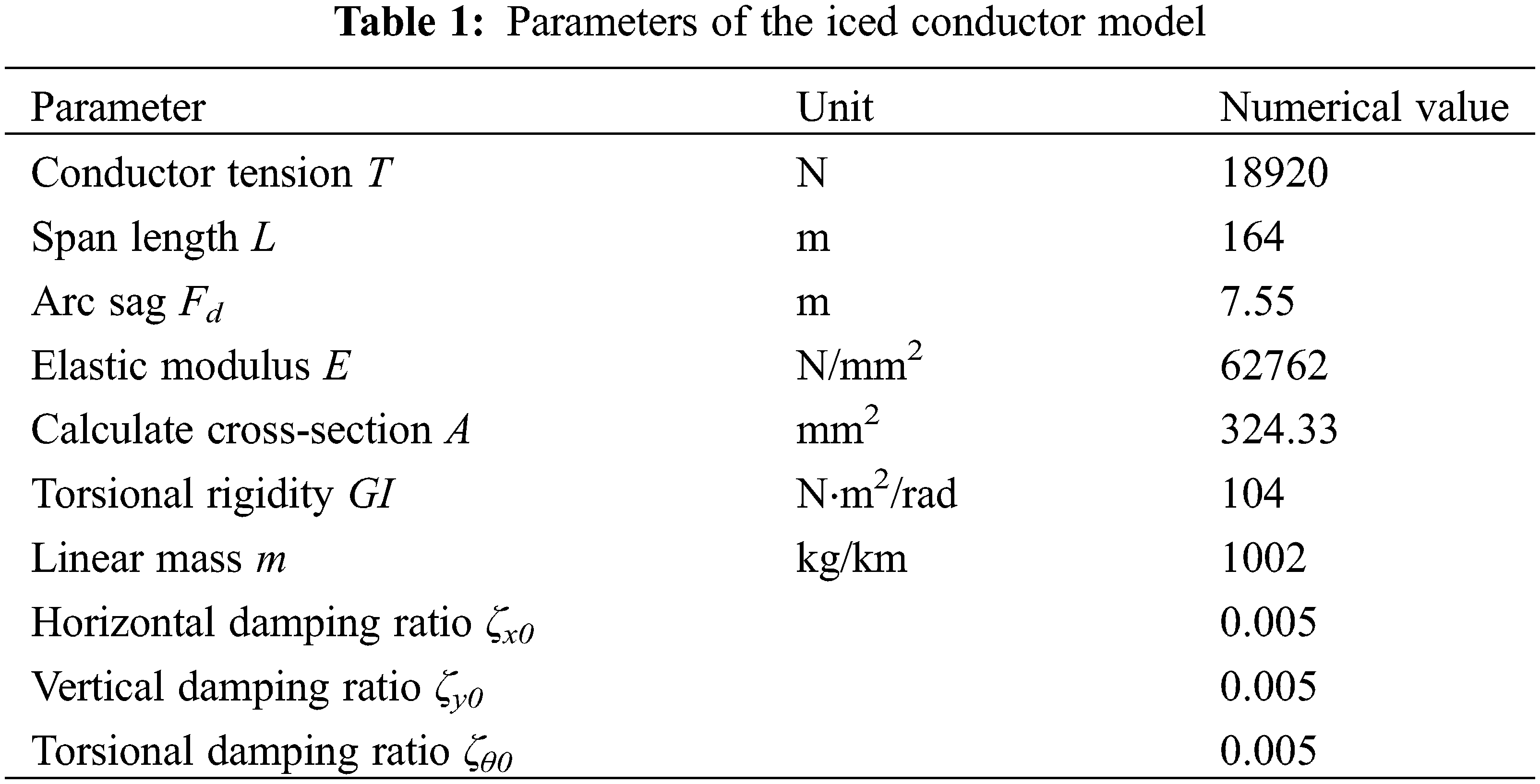
The flow field changes with the conductor boundary conditions and the movement of the conductor boundary in the flow field is realized using the overset mesh technology. In addition, the flow field domain mesh consists of a background mesh and an overset mesh. Background and overset meshes are both structured meshes, and the mesh height near the boundary layer of the conductor surface is less than 1 (y+ < 1), which can ensure the quality of the mesh. However, using the overset mesh technology, there is no need to worry about mesh distortion and mesh negative volume failing to solve. Thus, solving the overset mesh is as follows. First, the mesh around the conductor and the background mesh of the whole basin is divided, the boundary of the overset mesh is identified by the solver, and the overlapping part of the component mesh and the background mesh is “excavated”. Then, the boundary elements of the nested region are interpolated. The variable information of the boundary elements of the background region is also interpolated into the boundary elements of the nested region. Finally, the flow field is calculated to realize the fluid-solid coupling process. The computational mesh for the overall flow field is shown in Fig. 4c.

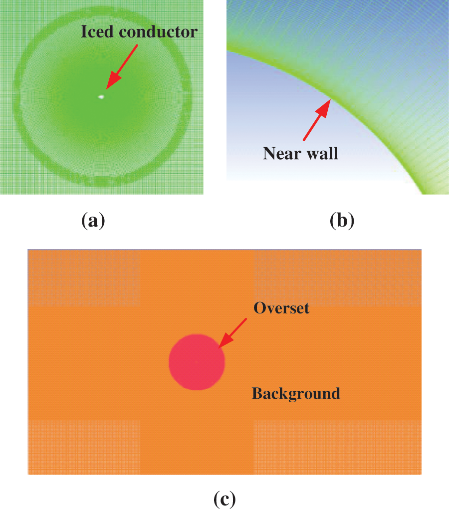
Figure 4: Computing domain meshing (a) Mesh nesting (b) Near wall mesh (c) Whole mesh

3.2 Calculation Parameters and Conditions

In the numerical simulation analysis, the air density is ρ = 1.225 kg/m3, the conductor is LGJ-300/20, the diameter is D = 23.43 mm, the quality of the iced conductor per unit length is m = 1002 kg/km, and the wind speed is U = 15 m/s. In this paper, the natural frequency of the iced conductor remains constant. Corresponding to the first-order natural frequency of the actual iced conductor with a span of L, the natural frequency of the iced conductor can be obtained by the theoretical calculation Eq. (18), and the natural frequency fn = 0.42 Hz is obtained. The time step is calculated by Eq. (19) to be 0.005 s. The parameter values used in the study are shown in Table 1.

fn=n2LTm (18)

Time step calculation equation [21]:

t=D/(U(10∼100)) (19)

where D is the wire diameter and U is the wind speed.

In the formula, m is the mass per unit length of the conductor, T is the tension of the conductor, n is the vibration order of the conductor, and L is the span of the conductor.

Fluent is only a purely computational mechanical calculation software and cannot directly solve the galloping response of the conductor structure. Therefore, it is necessary to write a corresponding program for the control equation of the iced conductor to solve the galloping response of the iced conductor to realize the fluid-solid coupling calculation of the iced conductor. Based on the governing equations of fluid dynamics, the structural dynamic response of an iced conductor is solved by the Runge-Kutta method. The dynamic update of the computational domain mesh is realized using dynamic and sliding mesh technology, and finally, the fluid-solid coupling solution of the iced conductor is realized. The flow chart of the structural dynamics of the iced conductor is shown in Fig. 5.

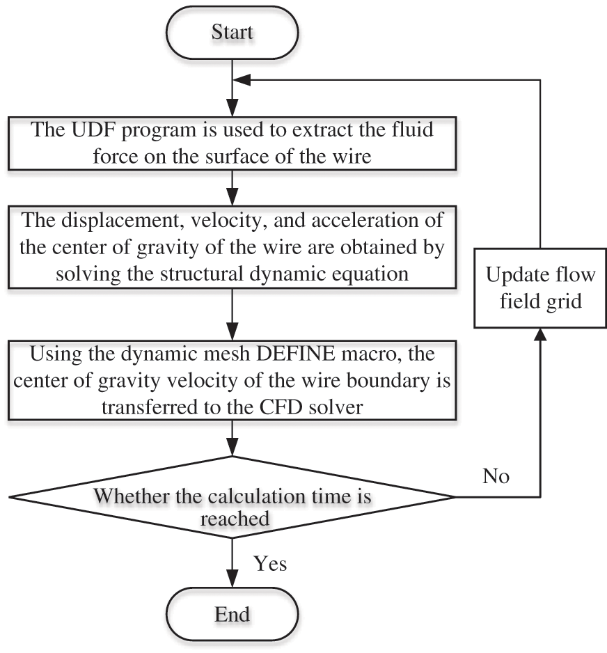
Figure 5: Solution process of structural dynamics

4  Numerical Results and Analysis

4.1 Aerodynamic Characteristics

To validate the applicability of the numerical calculation model proposed in this paper, Fig. 6 presents a comparison between the aerodynamic coefficients obtained from the numerical model and the wind tunnel test data from reference [11], using an iced conductor with a diameter of D = 26.82 mm and a thickness of 0.75D. Upon comparison, it can be observed that for a wind speed of 10 m/s and a turbulence intensity of Tu = 5%, the aerodynamic coefficients calculated by the numerical model in this paper exhibit a favorable agreement with the experimental results. This demonstrates the accuracy of the numerical calculation model presented in this paper and establishes a foundation for further investigation into the effects of different turbulence levels on the galloping phenomenon of iced conductors.

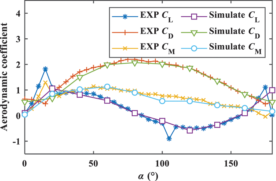
Figure 6: Aerodynamic coefficient of conductor with non symmetric shape

This paper analyzes the galloping response of iced conductors when turbulence intensity Tu = 5%, 15%, and 25% and the thickness of iced conductor is 0.5D. Fig. 7 shows the variation of the aerodynamic coefficient of the iced conductor with the windward angle. As shown in the figure, the turbulence intensity has little effect on the lift-drag characteristics and has a significant effect on the torsion coefficient. When the wind attack angle is small, the aerodynamic lift coefficient and torque coefficient of the iced conductor with turbulence intensity Tu = 15%, 25% have apparent peaks. Based on the mechanism of the Jacob Pieter Den Hartog galloping, galloping may occur in the range of wind attack angle with a negative slope of aerodynamic lift coefficient. Fig. 7b shows that the lift coefficient curve of the conductor has a negative slope in the range of 20°–60° and 110°–140° wind attack angle. Therefore, galloping may occur on the iced conductor within these two attack angles. In addition, if the torque coefficient of the conductor increases greatly, it will induce the galloping of the conductor. Meanwhile, Fig. 7c shows that when the turbulence model is 5% turbulence intensity, the torsion coefficient of the iced conductor fluctuates less and it is less affected by the turbulence model. However, with the increase of turbulence intensity in the turbulence model, the torsion coefficient of the iced conductor fluctuates more evidently. Therefore, the turbulence model significantly affects the torque of the iced conductor. Moreover, as shown in Fig. 7c, in the range of 0°–50° angle of attack, the torsion coefficient of the high turbulence model is significantly larger than that of the smaller turbulence model. Therefore, the turbulence model significantly affects the torsion coefficient of the iced conductor in the range of 0°–50°. It can be seen from the same figure that the turbulence intensity significantly affects the aerodynamic coefficient of the conductor in the range of 0°–50°. Iced conductors are more prone to galloping. This is primarily because the influence of turbulence intensity on the aerodynamic force of the conductor is mainly reflected in the following two aspects: first, the turbulence intensity changes the position of the airflow passing through the separation point on the surface of the iced conductor, and increases the contact range between the airflow and the conductor; second, turbulence increases the asymmetry of the fluid on the conductor surface and significantly increases the peak value of the torsion coefficient. In addition, when the wind attack angle of the iced conductor is in the range of 20°–50°, the iced conductor is more prone to galloping. It is because, in the range of 20°–50° angle of attack, the iced conductor is easily affected by the icing torque. Therefore, the conductor is more prone to galloping under icing conditions.

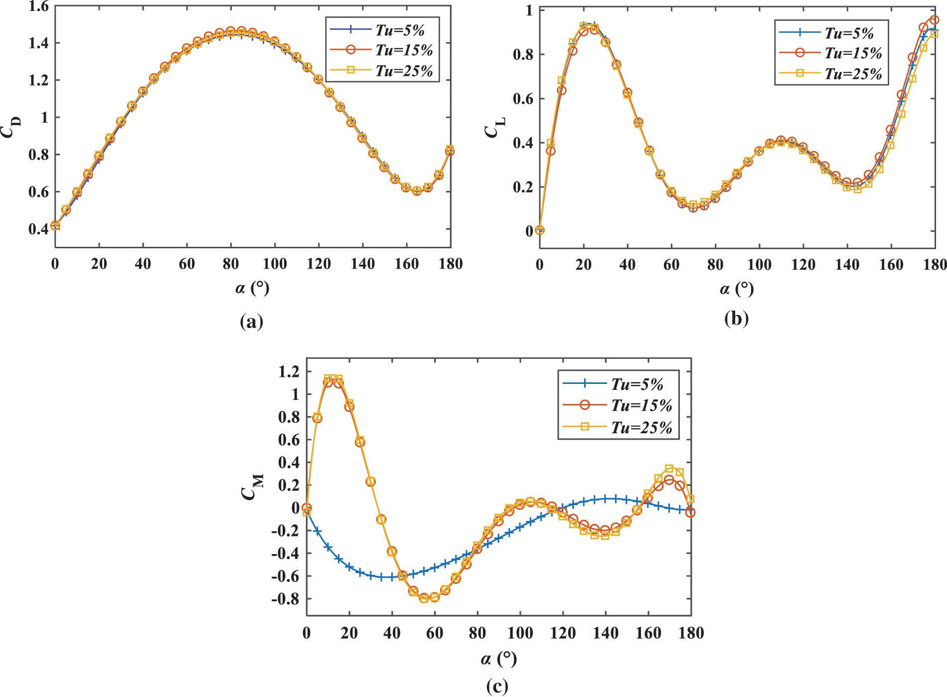
Figure 7: Aerodynamic characteristics of the iced conductor (a) Drag coefficient (b) Lift coefficient (c) Torsion coefficient

Fig. 8 shows the Den Hartog and Nigol coefficients of an iced conductor under different turbulence intensities. The unstable attack angle of the iced conductor is around 20°–80°. After icing on the windward side of the conductor, the wind attack angle can easily fall into the unstable range of 20°–80° under the torque generated by eccentric icing. Meanwhile, the increase of turbulence intensity in the wind field will also slightly reduce the Den Hartog coefficient and reduce the stability of the conductor. The absolute value of the Nigol coefficient and the range of unstable attack angle of the iced conductor increase with the increase of turbulence intensity. Among them, a 15% turbulence field has a more adverse effect on the stability of conductor relaxation. However, the absolute value of the Den Hartog coefficient decreases with the increase in turbulence intensity, which indicates that the increase in turbulence intensity will reduce the relaxation stability of an iced conductor to some extent.

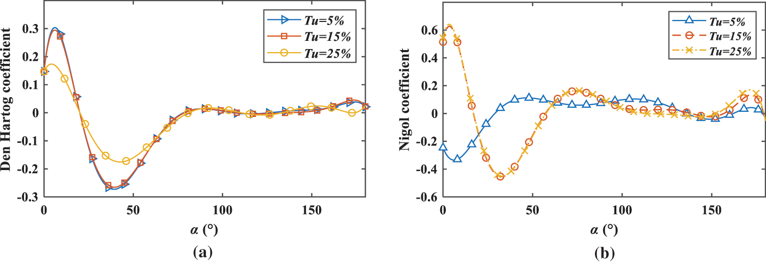
Figure 8: Den Hartog and Nigol coefficients of the iced conductor (a) Den Hartog coefficient; (b) Nigol coefficient

4.2 Galloping Characteristic

The aerodynamic coefficients of iced conductors greatly vary because of different turbulence intensities. In this paper, the galloping response of an iced conductor under different turbulence intensities was analyzed by the finite element method. Taking the single iced conductor as the research material, the ice thickness and the initial wind attack angle are 18 mm and 20°, respectively, and the influence of turbulence intensity on the galloping of the iced conductor was analyzed when the wind speed is 15 m/s. Fig. 9 shows the time history of the motion displacement of the iced conductor and the motion trajectory of the iced conductor when the turbulence intensity is 5%, 15%, and 25%. The flow direction displacement of the iced conductor under different turbulence intensities did not significantly change. The flow direction galloping amplitudes of the iced conductor under the three turbulence intensities were 0.76, 0.74, and 0.71 m, and the lateral amplitudes were 1.66, 2.09, and 2.17 m, respectively. The lateral amplitude slightly increased with the increase of turbulence intensity, and the torsion angle changed with the increase of turbulence intensity, thereby indicating that the large turbulence intensity may induce the line Nigel galloping. In addition, under different turbulence intensities, the galloping trajectories of the iced conductor do not change, and the trajectories of the iced conductor are slender and elliptical.

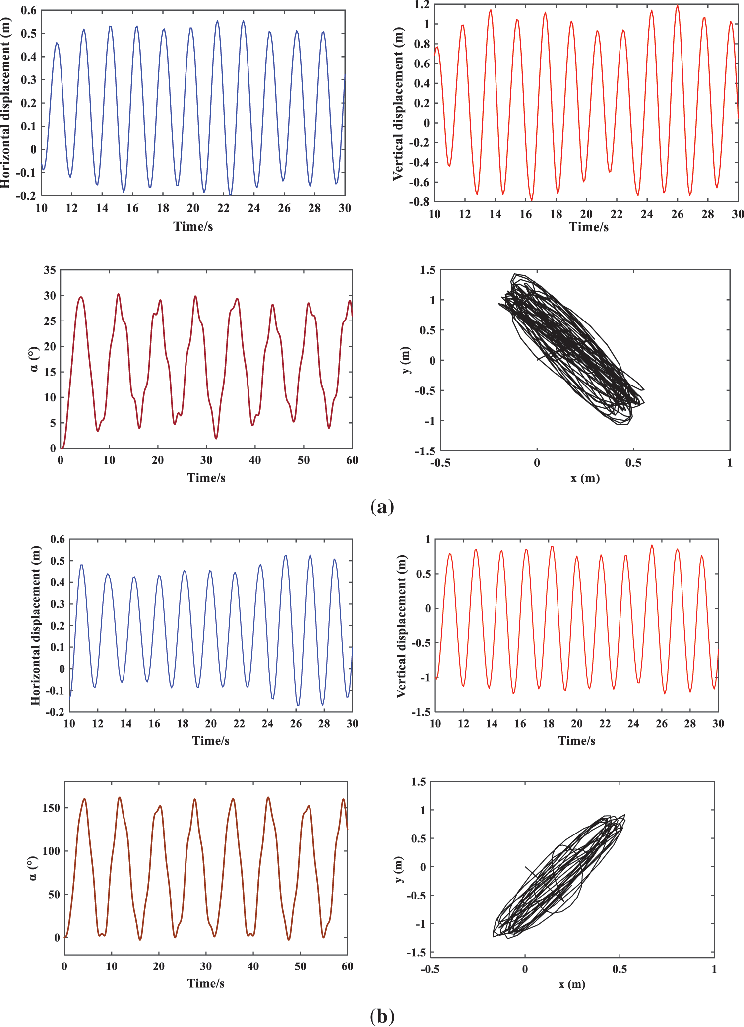
Figure 9: Galloping characteristics of the iced conductor (a) Tu = 5% (b) Tu = 15% (c) Tu = 25%

4.3 Influence of Wind Speed on the Galloping of the Iced Conductor

Based on the aerodynamic characteristics of iced conductors, the aerodynamic coefficients of iced conductors are different under different wind attack angles. From the negative slope of the lift coefficient, the unstable angle of attack of the lift coefficient of the iced conductor is in the range of 20°–60° and 110°–140°, and the torque coefficient has a large negative slope in the range of 20°–60° angle of attack. The iced conductor is prone to galloping. Generally, in actual situations, the initial wind attack angle of the line under natural wind is not greater than 90°. Therefore, this paper selected a typical wind attack angle of 20° for analysis. As shown in Fig. 10, when the wind attack angle is 20°, the horizontal, vertical, and torsional amplitudes of the iced conductor galloping increase with the increase of wind speed. At the same wind speed, the amplitude of the iced conductor galloping increases slightly with the increase of turbulence intensity, thereby indicating that the greater the wind speed, the more significant the influence of turbulence intensity on iced conductor galloping. When the wind speed is small, the turbulence intensity has little effect on the iced conductor galloping.

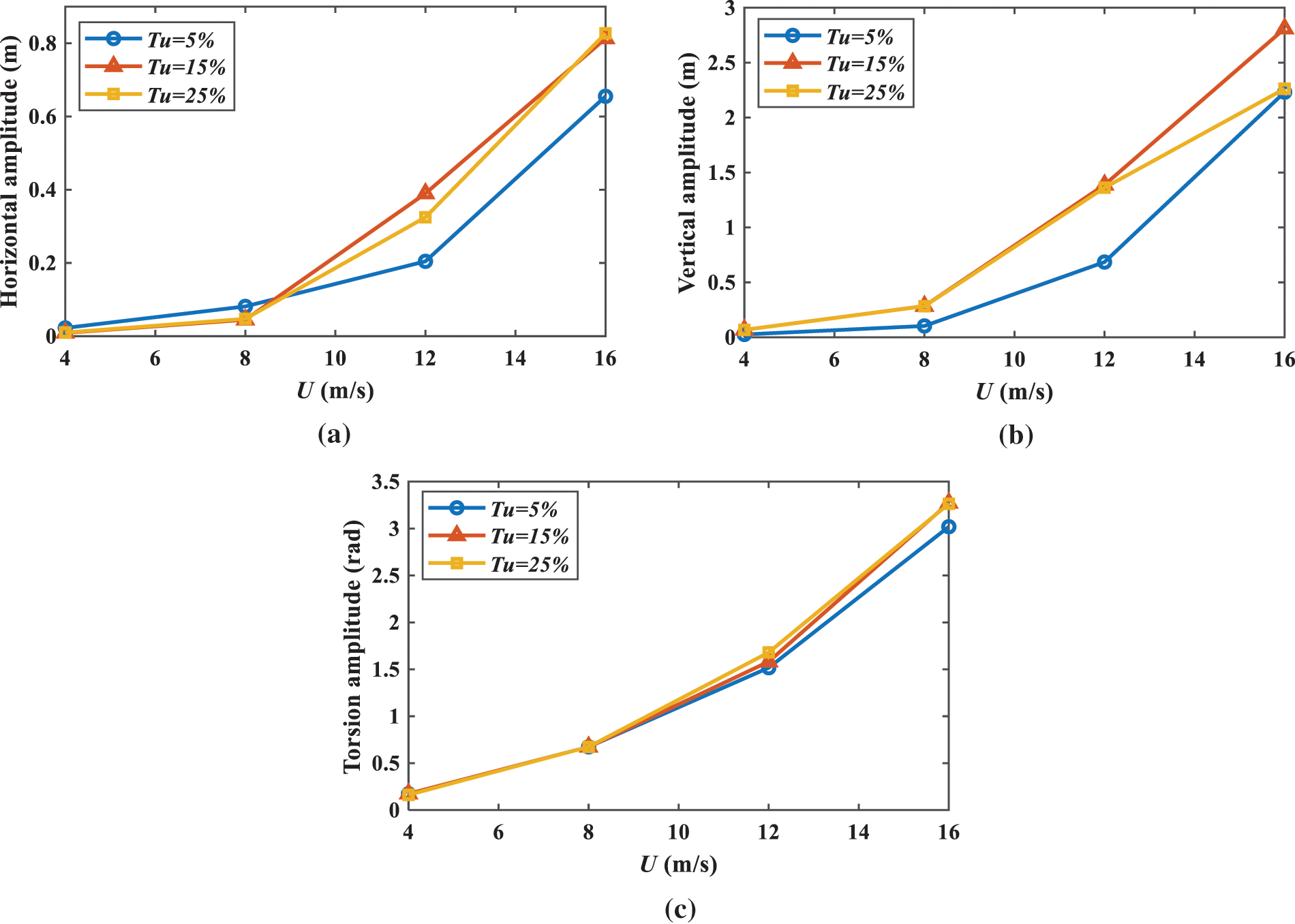
Figure 10: Maximum galloping amplitude of the iced conductors under different wind speeds (a) Horizontal amplitude (b) Vertical amplitude (c) Torsion amplitude

5  Conclusion

A nonlinear dynamic model of the fluid-solid coupling of a conductor with a non-symmetric shape is established in this paper. The variation of the aerodynamic coefficient of a conductor with a non-symmetric shape with the angle of attack under different turbulent environments is analyzed by aerodynamic theory. In addition, the variation of the galloping amplitude of a conductor with a non-symmetric shape with wind speed and turbulence intensity is analyzed. The main conclusions are as follows:

(1)   Turbulence intensity has little effect on the lift and drag coefficient of the iced conductor. The torsional coefficient of an iced conductor will suddenly increase at some angles of attack under turbulence. In addition, different wind attack angles will lead to significant differences in turbulence intensity and torsion coefficient of the iced conductor.

(2)   The amplitude of the iced conductor under different turbulence intensities is not much different. Thus, it is easier to induce the galloping of iced conductors and increase the angle of attack on iced conductors under turbulence. Moreover, under turbulent conditions, the trajectory of the iced conductor is slender and elliptical.

(3)   When the wind speed is large, the turbulence intensity has a significant effect on the galloping amplitude of the iced conductor. The larger the turbulence intensity, the larger the vertical and horizontal galloping amplitudes. The galloping amplitude of an iced conductor increases with the increase in wind speed.

Funding Statement: This work was supported in part by the National Natural Science Foundation of China [Grant No. 51867013].

Conflicts of Interest: The authors declare that they have no conflicts of interest to report regarding the present study.

References

1. Wang, L. M., Wang, Q., Lu, J. Z., Zhang, Z. H., Huang, T. (2019). Galloping characteristics of 500 kV iced quad bundle conductor. High Voltage Engineering, 45(7), 2284–2291. [Google Scholar]

2. Liu, Y., Cai, M. Q., Wang, Q. Y., Huang, C. L., Ding, S. L. et al. (2022). Investigation on the Sub-span oscillation in the process of galloping of iced eight-bundle conductors. Science Technology and Engineering, 22(12), 4843–4848. [Google Scholar]

3. Den, H. J. P. (1932). Transmission line vibration due to sleet. AIEE Transactions, 51(4), 1074–1076. [Google Scholar]

4. Nigol, O., Buchan, P. G. (1981). Conductor galloping 1: Den Hartog mechanism. IEEE Transactions on Power Apparatus and Systems, 100(2), 699–707. [Google Scholar]

5. Nigol, O., Buchan, P. G. (1981). Conductor galloping 2: Torsional mechanism. IEEE Transactions on Power Apparatus and Systems, 100(2), 708–720. [Google Scholar]

6. Yu, P., Shah, A., Popplewell, N. (1992). Inertially coupled galloping of iced conductors. Journal of Applied Mechanics, 59(1), 140–145. [Google Scholar]

7. Luongo, A., Zulli, D., Piccardo, G. (2007). A linear curved-beam model for the analysis of galloping in suspended cables. Journal of Mechanics of Materials & Structures, 2(4), 675–694. [Google Scholar]

8. Keutgen, R., Lilien, J. L. (2000). Benchmark cases for galloping with results obtained from wind tunnel facilities-validation of a finite element model. IEEE Transactions on Power Delivery, 15(1), 367–373. [Google Scholar]

9. Sansica, A., Loiseau, J. C., Kanamori, M. (2022). System identification of two-dimensional transonic buffet. AIAA Journal, 60(5), 3090–3106. [Google Scholar]

10. Diana, G., Manenti, A., Melzi, S. (2020). Energy method to compute the maximum amplitudes of oscillation due to galloping of iced bundled conductors. IEEE Transactions on Power Delivery, 36(5), 2804–2813. [Google Scholar]

11. Yan, D., Lu, Z. B., Lin, W., Lou, W. J. (2014). Experimental study on effect of turbulence intensity on the aerodynamic characteristics of iced conductors. High Voltage Engineering, 40(2), 450–457. [Google Scholar]

12. Chadha, J., Jaster, W. (1975). Influence of turbulence on the galloping instability of iced conductors. IEEE Transactions on Power Apparatus and Systems, 94(5), 1489–1499. [Google Scholar]

13. Renaud, K., Jean-Louis, L. (2000). Benchmark cases for galloping with results obtained from wind tunnel facilities-validation of a finite element model. IEEE Transactions on Power Delivery, 15(1), 367–374. [Google Scholar]

14. Shimizu, M., Ishihara, T. (2004). A wind tunnel study of aerodynamic characteristics of ice accreted transmission line. 5th International Colloquium on Bluff Body Aerodynamics and Applications, pp. 369–372. Ottawa, Canada. [Google Scholar]

15. Istvan, M. S., Yarusevych, S. (2004). Effects of free-stream turbulence intensity on transition in a laminar separation bubble formed over an airfoil. Experiments in Fluids, 59(3), 1–21. [Google Scholar]

16. Yang, X., Zhang, Z., Hao, S. Y. (2016). Dynamic aerodynamic characteristics of iced quad bundled conductors. Engineering Journal of Wuhan University, 49(4), 621–626+640. [Google Scholar]

17. Menter, F. R. (1994). Two-equation eddy-viscosity turbulence models for engineering application. AIAA Journal, 32(8), 1598–1605. [Google Scholar]

18. Li, X. L., Huo, B., Liu, X. J. (2021). Numerical simulation on galloping of iced conductor under uniformly decelerating wind field. Chinese Journal of Applied Mechanics, 38(2), 700–707. [Google Scholar]

19. Matsumiya, H., Yagi, T., Macdonald, J. H. G. (2021). Effects of aerodynamic coupling and non-linear behaviour on galloping of ice-accreted conductors. Journal of Fluids and Structures, 106, 103366. [Google Scholar]

20. Lou, W. J., Wang, L. Q., Chen, Z. F. (2022). Experimental study on aerodynamic characteristics of rime icing and glaze icing conductors. Journal of Vibration, Measurement & Diagnosis, 42(4), 684–689+823–824. [Google Scholar]

21. Chen, D. Y., Xiao, Q., Gu, C. J., Wang, G. P., Rui, X. T. (2020). Numerical calculation of vortex-induced vibration of a cylinder structure. Journal of Vibration and Shock, 39(19), 7–12+47. [Google Scholar]