Fluid-Structure Coupled Analysis of the Transient Thermal Stress in an Exhaust Manifold

1  Introduction

Using software simulations, Zhu et al. [1] calculated the temperature field and thermal stress distribution of an exhaust manifold by concentrating on cracks that appeared in the exhaust manifold of a specific gasoline engine during a thermal-shock test. Results of the analysis indicated that the cracks on the exhaust manifold were caused by high thermal stress. They subsequently optimized the manifold structure, thereby significantly reducing the thermal stress of the 4-2-1 exhaust manifold and eliminating the risk of cracks [1]. To ensure that an exhaust manifold worked properly under high temperature and normal circulation conditions, Deng et al. [2] established a fluid domain computational fluid dynamics (CFD) model and solid domain computer-aided engineering (CAE) model. These models simulated and analyzed the two-way fluid-solid coupling heat transfer of the tightly coupled exhaust manifold by using STAR-CCM+ fluid simulation software and ABAQUS finite element method (FEM) simulation software. Ultimately, they calculated the fluid outer wall temperature field, convective heat transfer coefficient field, and solid region temperature field [2]. In the study of Zheng et al. [3], the exhaust manifold of an engine worked improperly, making thermal stress and thermal load more likely to happen. As a result, deformation and subsequently fracture of the exhaust manifold occurred. Taking different inlet boundary conditions as objects, Zheng et al. analyzed the internal flow field temperature of the exhaust manifold and calculated the thermal stress and thermal deformation using the sequential fluid-structure coupling method. Higher intake temperatures and speeds resulted in greater thermal stress and thermal deformation at both the inlet and the outlet of the exhaust manifold [3]. Dong et al. used the direct coupling method to simulate the transient thermal fluid and thermal stress coupling of the engine exhaust manifold. They subsequently compared the difference between the transient calculation results and the steady-state calculation results and verified that the transient thermal fluid and thermal stress coupling simulation was more accurate than the steady-state calculation [4].

The CFD and FEM methods are already widely employed in thermal stress analyses of exhaust manifolds, and the accuracy of these models is steadily improving [5,6]. However, most studies utilize the steady-state method, which largely ignores transient analysis theory and often results in significant errors. Therefore, in this paper, we employ the coupled transient model using GT-POWER and STAR-CCM+ fluid software and apply it to the exhaust manifold of a gasoline engine as the research object. The GT-POWER software transmits the inlet boundary information (mass flow and temperature) under transient conditions to STAR-CCM+ using UDF files in real-time. This ensures that the inlet mass flow and temperature change accordingly with variations in crankshaft angle, thus improving the accuracy and reliability of the calculated results. Devising an approach that accurately calculates the temperature field and thermal stress of exhaust manifolds provides a valuable reference for further research into gasoline engine exhaust manifolds.

2  Fluid-Structure Coupled Mode

Fluid-solid coupling heat transfer refers to the interaction between solids and fluids, accompanied by heat exchange. Therefore, it involves the joint action of mechanical load and thermal load. When coupling data is extracted from the coupling interface between the solid domain and the fluid domain, the solid domain uses the oil film temperature and heat transfer coefficient transmitted by the fluid, while the fluid uses the wall temperature transmitted by the solid domain as the boundary condition [7]. In the transient solution, accurate dynamic boundary conditions are particularly important. In this paper, we verify the combustion performance and emission characteristics of the one-dimensional simulation model engine experimentally, thereby proving the effectiveness of the simulation model [8].

In order to accurately obtain the temperature distribution, flow characteristics and the thermal stress distribution on the solid wall of the exhaust manifold. The temperature variation, the turbulent mixing, the transport of fluid components and the convection diffusion should also be taken into account when establishing the mathematical model. The basic governing equations of the fluid domain include the energy conservation equation, the momentum conservation equation and the mass conservation equation.

The mass conservation equation is given by [9–11]

∂ρ∂t+∂∂xi(ρui)=0 (1)

where t is the time, ui is the velocity component in the xi direction, ρ is the density of the fluid.

The momentum conservation equation is given by

∂∂t(ρui)+∂∂xi(ρuiuj)=∂ρ∂xi+∂τij∂xj+ρgi (2)

where ρgi is the component of gravity in the i direction, ρ is the static pressure, τij Is the stress vector.

The energy conservation equation is given by

∂∂t(ρh)+∂∂xi(ρuih)=∂∂xi(k+ki)∂T∂xi (3)

where ki is the conductivity caused by turbulent transfer, h is the static enthalpy, and k is the molecular conductivity.

Due to heat transfer between the fluid and the solid wall, the exhaust manifold needs to be divided into the fluid and solid domains [12]. The boundary conditions of the fluid domain are used to generate data for the inner surface of the cavity in the geometric model. An interface is generated between the solid domain and the fluid domain, where the contact surface between the two domains is defined as a type of heat and mass transfer. The solid mesh model is a combination of polyhedron and thin-film mesh models, which meets the requirements of computational accuracy [13]. The STAR-CCM+ unique polyhedron grid is used in the grids of the two domains, thus effectively reducing the number of grids and enhancing the utilization of computing resources [14].

In the fluid domain, the k - ε turbulence model is used to calculate the convective heat transfer between fluid and wall as the boundary condition. The transport equation of standard k - ε turbulence model can be described as

∂∂t(ρk)+∂∂xi(ρkui)=∂∂xj[(μ+μtσk)∂k∂xj]+Gk+Gb−ρε−YM+Sk (4)

∂∂t(ρε)+∂∂xi(ρεui)=∂∂xj[(μ+μtσε)∂ε∂xj]+G1εεk(Gk+G3εGb)−G2ερε2k+Sε (5)

where k is the turbulent kinetic energy, ε is the turbulent dissipation rate, Gk is the turbulent kinetic energy term generated by average velocity gradient, Gb is the turbulent kinetic energy term generated by buoyancy, YM is the expansion dissipation term, G1ε , G2ε , G3ε are constant. σk and σε are Prandtl numbers of k and ε . Sk and Sε are user-defined source items.

There are three basic methods for heat transfer: thermal conduction, thermal radiation and thermal convection. Thermal convection widely exists in various fluids, it refers to the process of heat transfer between various parts of the fluid due to relative displacement. The heat transfer that causes heat movement is called thermal conduction. Thermal radiation is electromagnetic radiation generated by the thermal motion of particles in matter. Thermal radiation is generated when heat from the movement of charges in the material is converted to electromagnetic radiation. In this paper, the effect of thermal radiation is ignored because it has little effect on this study [15].

Thermal conduction follows Fourier law is given by

q=−λ∂T∂n (6)

where q is the heat flux density, λ is the thermal conductivity, ∂T∂n is the temperature gradient in all directions.

Thermal convection equation can be described as

q=hf(Ts−TG) (7)

where hf is the convective heat transfer coefficient, Ts is the surface temperature of solid. TG is the fluid temperature.

Assuming that the manifold is a circular tube, the convective heat transfer coefficient between the high-temperature exhaust gas and the inner wall surface is given by

hf=Nuλf/d0 (8)

where d0 is the inner diameter of exhaust branch pipe, λf is the thermal conductivity of the gas, Nu is the Nusselt number. Due to Re>104 , Nu=0.023Re0.8Prf0.3 , Re=Ud0/rf , Prf is the Prandtl number, U is the average flow rate of gas in the pipe, rf is the Kinematic viscosity of gas.

Physical models are often divided into a large number of units in finite element analysis. The governing equation of thermal conduction of the unit body can be written as follows:

∂∂x(λxx∂T∂x)+∂∂y(λyy∂T∂y)+∂∂z(λzz∂T∂z)+q=ρcdTdt (9)

where

dTdt=∂T∂t+Vx∂T∂x+Vy∂T∂y+Vz∂T∂z

Vx , Vy and Vz are the medium conductivity.

2.1 Sub-Model

By utilizing a combination of GT-POWER and STAR-CCM+ fluid software, the inlet boundary conditions (Inlet mass flow of the four cylinders and gas temperature at the four cylinder inlets) solved by GT-POWER are transferred to STAR-CCM+ in real-time under transient conditions. Then the node temperature of the temperature field distribution in the fluid domain is calculated by STAR-CCM+. The node temperature is directly defined by some commands, and then it is used as the body load as the input to solve the wall thermal stress.

The STAR-CCM+ program has a variety of built-in physical models. The Three-Dimensional model is selected to represent space and the Implicit Unsteady model is chosen for time. Through analysis of the geometric model, we can see that large memory resources are required for performing calculations using the model. Therefore, to reduce the number of calculations, we select Segregated Flow as the flow item. Since the Reynolds number of the gas in the engine exhaust manifold is greater than 2300, the flow state of the gas in the exhaust manifold is three-dimensional turbulent flow. The k- ε model is the most widely used turbulence model in the industry, so we choose the k - ε turbulence model for this study. Due to the strong turbulent flow of gas in the exhaust manifold, we set the turbulence intensity to 0.1 and the vortex scale to 0.05 of the inlet radius. The sub-model selection is listed in Table 1.

2.2 Initial Conditions

To facilitate CFD transient analysis, the parameters of the calculation domain and the wall boundary parameters at zero time are set as the initial conditions of the analysis. The setting of these parameters has a substantial impact on the convergence of the model and the accuracy of the calculation results. Therefore, the initial conditions of the thermal analysis flow field are: initial pressure of 1.01 × 105 N/m2; ambient initial temperature set at 300 K; initial velocity of 0 m/s; and the convective heat transfer coefficient of the outer wall of the exhaust manifold is 11 W/m2∙k). The values of constants are listed in Table 2.

2.3 Boundary Conditions

According to the design parameters of engines and exhaust manifolds shown in Table 3, we construct a one-dimensional simulation model for naturally aspirated gasoline engines using GT-POWER software with an ignition sequence of 1-3-4-2, four cylinders, and four strokes. The model includes an intake and exhaust system, oil supply system, cylinder block system, as well as other modules. The one-dimensional simulation model of the engine is built using GT-POWER software, as Fig. 1 illustrates. This model provides the boundary conditions of the inlet and outlet of the engine exhaust manifold.

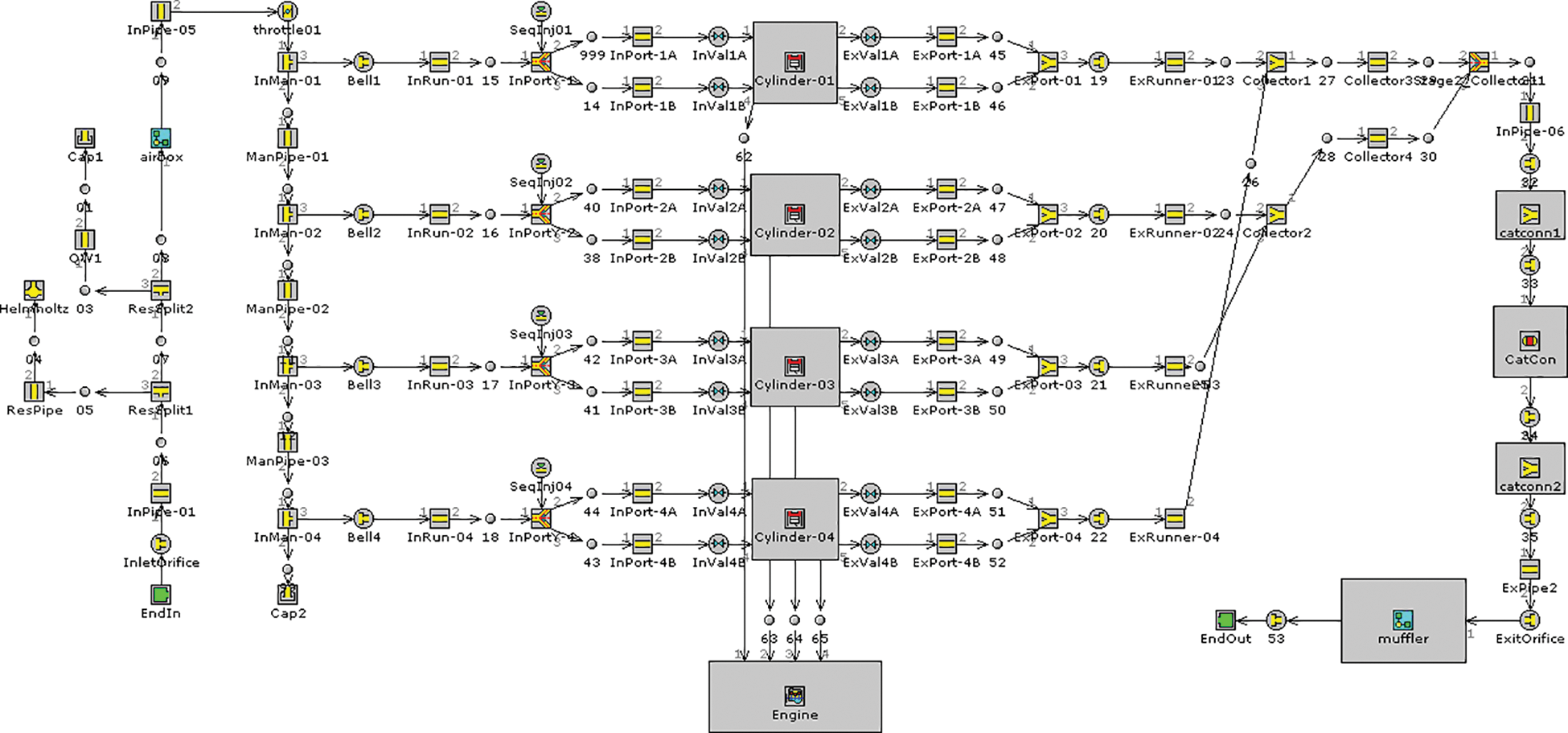
Figure 1: One-dimensional simulation model of engine

When the exhaust manifold works, the internal air flow and solid wall heat transfer change dynamically with time. In order to avoid the non convergence of the exhaust manifold in the first cycle, the transient calculation of the exhaust manifold for three cycles (2160°CA) is carried out in this paper. Because the time of each crank angle is 3.3 × 10−5 s under the maximum speed of 5000 r/min, the time step is set to 3 × 10−5 s. The maximum iteration number is set to 10, which can ensure the full transmission of data between nodes.

In this study, we compare the external characteristic curve of the engine with that of the one-dimensional simulation model. Then, we gradually modify the parameters of the simulation model until the external characteristic curve calculated by the one-dimensional simulation model is in good agreement with the experimental value. As Figs. 2 and 3 indicate, the errors for power and torque between the simulation and test are 3.7% and 2.8%, respectively. These values are both within 5%, which verifies the effectiveness of the GT-POWER simulation model.

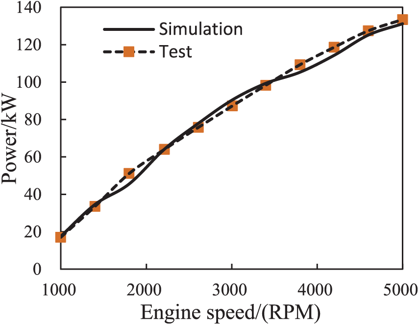
Figure 2: Results of power simulation and test

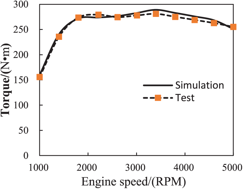
Figure 3: Results of torque simulation and test

According to the calculations of the GT-POWER simulation, we obtain values for the inlet mass flow and gas temperature at the four cylinder inlets, as Figs. 4 and 5 show, respectively. In the coupling simulation between GT-POWER and STAR-CCM+, GT-POWER transfers the entry boundary conditions to STAR-CCM+ in real-time in the form of a UDF file.

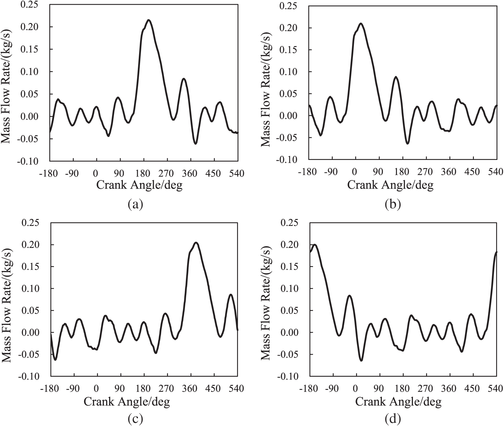
Figure 4: Inlet mass flow of the four cylinders

Figure 5: Gas temperature at the four cylinder inlets

2.4 Grid Independence Verification

The instantaneous velocity in engine exhausts can reach hundreds of meters per second, with high Reynolds numbers. This produces non-negligible viscous forces, and the velocity gradient is very large along the normal direction. Therefore, to ensure the accuracy of the calculation results and capture the flow characteristics in this region more effectively, it is necessary to divide the boundary layer. In this paper, the target y+ value is 30, and a three-layer boundary layer grid with a thickness of 0.56 mm is generated on the interface between fluid domain and solid domain by calculation.

Taking the exhaust manifold inlet wall temperature as the evaluation index, we compare the modeling results of 0.91 million, 1.12 million, 1.44 million, and 2.04 million grids. Ultimately, we select 1.12 million grids as the optimal value. Of the total number of 1.12 million grids, 0.32 million are in the fluid domain, while 0.8 million are in the solid domain, as Fig. 6 displays. The mixing factor, growth factor, and density of the tetrahedrons and polyhedrons are all set to 1.2. An appropriately-sized grid ensures sufficient data transmission between nodes during calculations. Thus, the global and minimum grid sizes are 1.5 and 0.5 mm, respectively.

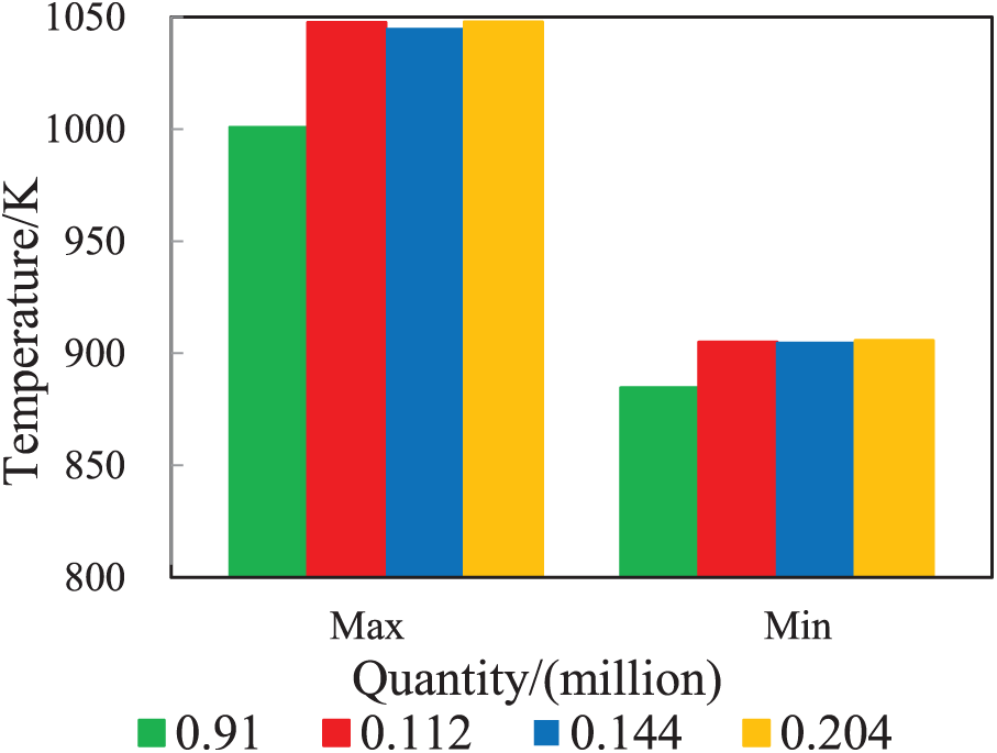
Figure 6: Effect of grid number on exhaust manifold temperature

2.5 Temperature Field Analysis

The temperature distribution in the solid domain of the manifold has a tremendous impact on the thermal stress and thermal deformation of the entire exhaust manifold. This can, as a result, seriously affect the service performance and service life of the exhaust manifold [20]. As Figs. 7 and 8 illustrate, the maximum temperature of the outer wall of the exhaust manifold appears in the upper area of the pressure stabilizing chamber at the outlet end, reaching 1047.7 K, which is similar to the temperatures at the intersection of the second and third branch pipe outlets. This high temperature is mainly attributable to the rapid vortex collection of high-temperature gas in the exhaust manifold. Additionally, the surface of the four inlet flanges is not in direct contact with high-temperature airflow. Besides, there is a large heat dissipation area and little fluid heat transfer, resulting in lower temperatures. The temperature at the outlet flange is higher than at the inlet flange, but the minimum temperature is only 905 K.

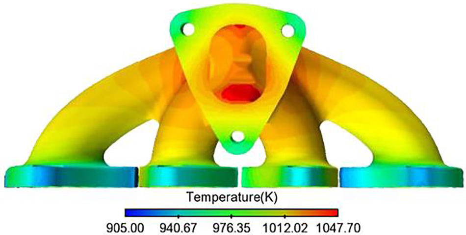
Figure 7: Exhaust manifold outer wall temperature (front)

Figure 8: Exhaust manifold outer wall temperature (rear)

The outer wall surface of the exhaust manifold directly generates convective heat transfer with the external environment, so the temperature is relatively low. In contrast, the inner wall surface is in direct contact with high-temperature gas, resulting in high convective heat transfer intensity and temperature. Moreover, the temperature range in the exhaust manifold wall surface is unevenly distributed, and there is a certain temperature gradient between the inner and outer wall surfaces. The maximum wall temperature of the exhaust manifold is shown in Fig. 8, where the wall thickness is 5.5 mm. At the node with the maximum temperature, we place a monitoring point every 0.5 mm from the inside to the outside along the radial direction of the wall surface. A total of 11 points from the outer wall surface to the inner wall surface are used to analyze the temperature variations at the node with the maximum temperature, as shown in Fig. 9.

Figure 9: The temperature of the solid wall at the node with the maximum temperature

3  Thermal Stress Model

3.1 Boundary Conditions

The thermal deformation and thermal stress of the structure can be calculated by adding appropriate figures to the model for solving the temperature field. First, the temperature field in the solid domain is used as the applied load for thermal stress analysis, then the thermal deformation and thermal stress of the structure are calculated by the load step of the static analysis. The nonlinear parameters of the material are set according to the temperature variation range. Besides, the material of the exhaust manifold wall is QTANi35si5Cr2. Mechanical properties of the material include a yield strength greater than 220 MPa and a tensile strength greater than 370 MPa. Other material property parameters are presented in Table 4. The boundary condition is to constrain all degrees of freedom in the bolt holes at the front and rear flanges, while the ambient temperature is set to 300 K.

3.2 Thermal Stress and Thermal Deformation

As Fig. 10 shows, a maximum thermal deformation of 1.64 mm occurs at the bending position of the pipelines of Cylinder 1 and Cylinder 4. Fig. 11 indicates that maximum thermal stress occurs at the junction between the outlet flange and the manifold. The maximum value is 205.03 MPa, which exceeds the yield strength of the material (200 MPa). Therefore, irrecoverable plastic deformation occurs near this position. Besides, there is a large temperature gradient at the junction between the outlet flange and the manifold. This position is more prone to thermal expansion and cold contraction during the temperature cycle, thus leading to large thermal stress and a greater likelihood of fatigue failure. Here, the local shape is maintained and the mesh is encrypted, resulting in excessive rough mesh and large thermal stress concentration. In practical situations, engineers should consider measures to reduce stress concentration during design and manufacturing, such as by setting chamfer. Results from the analysis also indicate that stress concentration occurs at the junction between the inlet flange and the branch pipeline, but it is less than the yield strength.

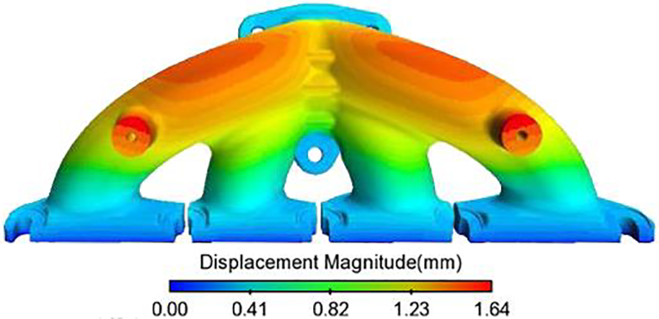
Figure 10: Cloud diagram of thermal deformation

Figure 11: Cloud diagram of thermal stress

3.3 Optimization Measures

In this paper, we improve the original manifold model by strengthening the connecting rib plate to increase the overall stiffness of the manifold. The purpose of this is to reduce the thermal stress at the exhaust manifold without changing the internal flow field, thereby making the stress in the exhaust manifold more uniform and increasing overall structural stiffness. The improved model is displayed in Fig. 12.

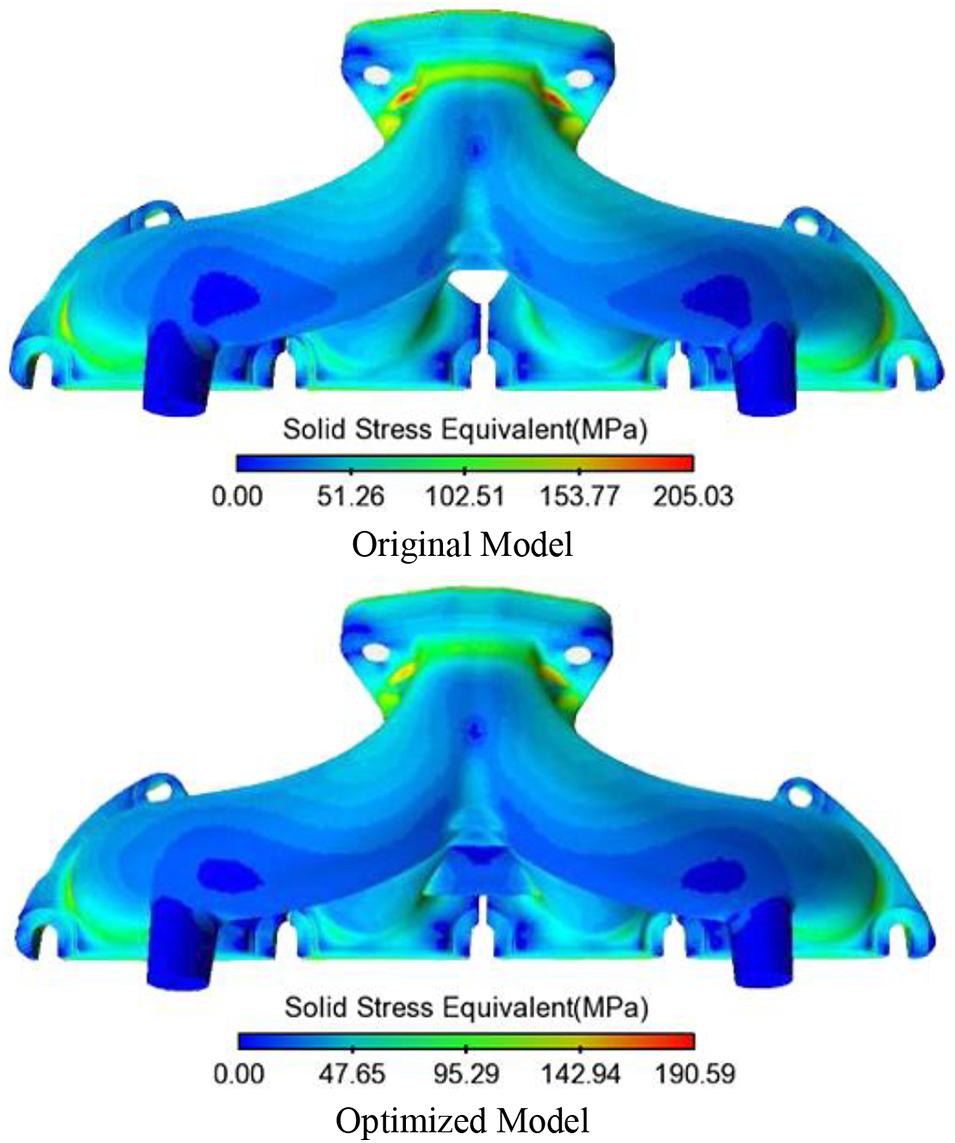
Figure 12: Cloud diagram of thermal stress before and after optimization

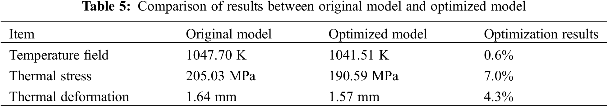
Fig. 12 shows a thermal stress comparison between the optimized model and the original model, and it reveals that the overall thermal stress distribution trend in the manifold remains essentially unchanged. However, the stress value decreases to a certain extent compared with before improvements. This is especially true at the junction between the exhaust manifold outlet and the flange, as well as the junction of each exhaust manifold branch pipe. The maximum thermal stress is reduced by up to 14.44 MPa from 205.03 to 190.59 MPa, indicating a decrease of about 7.0%. After optimization, the maximum thermal stress is within the yield strength of the material (200 MPa), thus meeting service requirements.

The maximum thermal strain decreases from 1.64 to 1.57 mm, primarily because the connecting ribs between the branch pipes somewhat restrict the deformation of the exhaust manifold, where the maximum thermal strain decreases by 0.07 mm, which is a 4.3% reduction.

To highlight the differences between the original model and the improved model, Table 5 lists the results of the calculations. It indicates that there is a general consistency between the original model and the improved model regarding the distribution of temperature field, thermal stress, and thermal deformation. However, the calculated values are slightly different, and the maximum temperature of the improved model is about 6.19 K lower than the original model. While this change is negligible, the thermal stress and thermal deformation decrease more significantly.

4  Conclusions

In this study, we established a one-dimensional model of the engine using GT-POWER software, then completed a calibration verification of the model. After calibration, the errors regarding torque and power between the simulation and the test were 2.8% and 3.7%, respectively. Coupled with STAR-CCM+ software, GT-Power calculated fluid-structure coupling with inlet temperature and mass flow rate as boundary conditions, thereby solving the problem of setting dynamic boundary conditions in a transient analysis. The temperature field of the exhaust manifold wall under actual working conditions was obtained by directly analyzing coupled heat transfer. According to the calculation results of thermal stress and thermal deformation under a transient temperature field, we optimized the original model by adding connections. After optimization, the maximum thermal stress fell by 14.44 MPa, or 7.0%, which demonstrates that the optimization scheme is feasible. These results provide a useful reference for optimizing designs of gasoline engine exhaust manifolds.

Funding Statement: This work is supported by the Basic Ability Improvement Project for Young and Middle-Aged Teachers in Guangxi Universities, Project No. 2021KY0792.

Conflicts of Interest: The authors declare that they have no conflicts of interest to report regarding the present study.

References

1. Zhu, Q., Yuan, Z. C., Ma, J. Y., Li, S. Y., Huang, K. et al. (2013). Thermal analysis for the exhaust manifold of a supercharged gasoline engine based on fluid-solid coupling. Automotive Engineering, 35(12), 1134–1138+1133. [Google Scholar]

2. Deng, G. H., Li, H. B., Yang, E. C., Zhu, Z. Y. (2018). Research on thermal stress analysis method for tight coupling exhaust manifold. Journal of Chongqing University of Technology (Natural Science), 32(4), 41–47. [Google Scholar]

3. Zheng, X. J., Chen, J. Q., Lan, F. C., Zhang, X. D. (2017). The fluid-solid coupling thermal analysis on an engine exhaust manifold. Machine Design and Manufacturing Engineering, 46(12), 13–17. [Google Scholar]

4. Dong, F., Cai, Y. X., Fan, Q. Y., Jiang, S. L., Guo, C. H. (2010). A study on the transient thermal fluid and thermal stress coupled simulation for the exhaust manifold of ice. Automotive Engineering, 32(10), 854–859. [Google Scholar]

5. Sugiyama, K., Ii, S., Takeuchi, S., Takagi, S., Matsumoto, Y. (2011). A full Eulerian finite difference approach for solving fluid-structure coupling problems. Journal of Computational Physics, 230(3), 596–627. [Google Scholar]

6. Li, B., Cui, Y., Fu, Y., Deng, K., Tian, Y. et al. (2022). Marine diesel exhaust manifold failure and life prediction under high-temperature vibration. Proceedings of the Institution of Mechanical Engineers, Part C: Journal of Mechanical Engineering Science, 236(11), 6180–6191. https://doi.org/10.1177/09544062211064957 [Google Scholar]

7. Li, D. L., Yin, Y. F., Chen, G. F., Cui, C., Han, B. (2012). Thermal fatigue analysis of the engine exhaust manifold. Advanced Materials Research, 482–484, 214–219. https://doi.org/10.4028/www.scientific.net/AMR.482-484.214 [Google Scholar] [CrossRef]

8. Goga, G., Chauhan, B. S., Mahla, S. K., Dhir, A., Cho, H. M. (2020). Effect of varying biogas mass flow rate on performance and emission characteristics of a diesel engine fuelled with blends of n-butanol and diesel. Journal of Thermal Analysis and Calorimetry, 140(6), 2817–2830. https://doi.org/10.1007/s10973-019-09055-1 [Google Scholar]

9. Benek, G., Ozsoysal, O. A. (2021). Influences of the dead end on the flow characteristics at the exhaust manifold of a marine diesel engine. Journal of Thermal Engineering, 7(6), 1519–1530. [Google Scholar] [CrossRef]

10. Ancellin, M., Brosset, L., Ghidaglia, J. M. (2020). On the liquid-vapor phase-change interface conditions for numerical simulation of violent separated flows. Fluid Dynamics & Materials Processing, 16(2), 359–381. https://doi.org/10.32604/fdmp.2020.08642 [Google Scholar]

11. Najibi, A., Alizadeh, P., Ghazifard, P. (2021). Transient thermal stress analysis for a short thick hollow FGM cylinder with nonlinear temperature-dependent material properties. Journal of Thermal Analysis and Calorimetry, 146(5), 1971–1982. https://doi.org/10.1007/s10973-020-10442-2 [Google Scholar] [CrossRef]

12. Celikten, B., Duman, I., Harman, C., Eroglu, S. (2018). Exhaust manifold thermal assessment with ambient heat transfer coefficient optimization. SAE International Journal of Passenger Cars-Mechanical Systems, 11(3), 193–202. https://doi.org/10.4271/06-11-03-0016

13. Liu, Z., Wang, X., Zhang, Y., Li, X., Xu, Y. (2014). Study on the unsteady heat transfer of engine exhaust manifold based on the analysis method of serial. SAE International Journal of Engines, 7(3), 1547–1554. https://doi.org/10.4271/2014-01-1711

14. Liu, Z., Chen, J., Xiao, S. (2016). Thermo-mechanical fatigue study of gasoline engine exhaust manifold based on weak coupling of CFD and FE. SAE Technical Paper, 2016-01-2350. https://doi.org/10.4271/2016-01-2350

15. Yong, S., Bin, L., Shanquan, L., Xiaojun, Y. (2013). Fluid-solid coupling simulation on engine exhaust manifold. Computer Aided Engineering, 22(S2), 91–94. https://doi.org/10.3969/j.issn.1006-0871.2013.z2.023

16. Partoaa, A. A., Abdolzadeh, M., Rezaeizadeh, M. (2017). Effect of fin attachment on thermal stress reduction of exhaust manifold of an off road diesel engine. Journal of Central South University, 24, 546–559. https://doi.org/10.1007/s11771-017-3457-1

17. Prakash, C. M., Sourav, K. K., Harshit, M. (2018). Effect of perforation on exhaust performance of a turbo pipe type muffler using methanol and gasoline blended fuel: A step to NOx control. Journal of Cleaner Production, 183, 869–879. https://doi.org/10.1016/j.jclepro.2018.02.236

18. Sorin, A., Bouloc, F., Bourouga, B., Anthoine, P. (2008). Experimental study of periodic heat transfer coefficient in the entrance zone of an exhaust pipe. International Journal of Thermal Sciences, 47(12), 1665–1675. https://doi.org/10.1016/j.ijthermalsci.2008.01.006

19. Uang, Z. H., Huang, J. R., Tang, X. L. (2020). On fluid-solid coupling thermal simulation analysis of exhaust manifold. Journal of Southwest China Normal University (Natural Science Edition), 45(6), 107–112. https://doi.org/10.13718/j.cnki.xsxb.2020.06.016

20. Liu, S., Leng, L., Zhou, W., Shi, L. (2021). Optimizing the exhaust system of marine diesel engines to improve low-speed performances and cylinder working conditions. Fluid Dynamics & Materials Processing, 17(4), 683–695. https://doi.org/10.32604/fdmp.2021.013575