Analysis of Wellbore Flow in Shale Gas Horizontal Wells

1  Introduction

Shale reservoir is characterized by extremely low porosity and very low permeability, self-generation and self-storage. Horizontal wells and large-scale fracturing stimulation technologies are usually used to develop shale gas reservoirs, and the cluster well development mode is adopted. Multiple horizontal wells with different bottom extension directions are arranged on one platform. A large amount of liquid is injected into the formation during fracturing. With the continuous extraction of shale gas, the pressure and gas production of the gas well is getting lower and lower, and the liquid-carrying capacity of wellbore is weakened, which leads to the risk of liquid loading or even water flooding at any time. It is of great significance to understand the gas-liquid two-phase flow of shale gas well, which is beneficial to determine reasonable tubing running depth or design artificial lift, further improve the liquid-carrying capacity of gas well and develop shale gas efficiently.

Numerous scholars have investigated the characteristics of gas-liquid two-phase pipe flow in conventional gas wells, including wellbore gas-liquid two-phase flow pattern, liquid holdup model and pressure drop model, etc. Williams [1] proposed a method of predicting the type of two-phase flow in wellbore of a gas well using a program written in FORTRAN, Bill-FlowTRAN.f95 (the flow regimes covered are mist, transition, and slug flow). Lina et al. [2] evaluated the best correlation of 63 different void fraction models under specific conditions. Mansour et al. [3] obtained a new correlation for bubble migration length to the upper pipe wall. Kim et al. [4] derivated a new slug flow model to calculate the pressure gradient for horizontal and near horizontal pipes.

However, due to the characteristics of shale gas wells, such as variable wellbore trajectory, long horizontal section and different liquid production sources, the wellbore flow is complex, and a single method is not enough to describe the flow features of all shale gas wells. In particular, the misjudgment of flow would inevitably lead to an erroneous prediction of gas well performance [5]. According to the literature, more researchers focus on the two-phase flow in shale gas reservoirs [6–8]. Regarding gas and liquid distribution characteristics in the wellbore, Li [9] and He et al. [10] used a numerical simulation to study the wellbore flow of shale gas horizontal well and recognized that the deflection is the most difficult to carry liquid. Yu et al. [11], through an indoor experiment, further proved that 55° is the most challenging liquid carrying point, and concluded that 60°~70° is the best target well section for implementing drainage and gas production technology. In terms of wellbore pressure distribution, Liu et al. [12] compared the pressure calculated by the six commonly used pressure calculation models with the measured pressure of a single well and found that the Mukherjee & Brill model gave the smallest calculation error. Similarly, Liu [13] used 50 groups of measured pressure data of shale gas wells to evaluate and optimize six commonly used pipe flow models. With 45° as the limit, when the well deviation angle is less than or equal to 45°, the Hagedorn & Brown Revised model is more applicable; Otherwise, Beggs & Brill Revised model is recommended. Xie et al. [14] proposed a new pressure drop calculation model suitable for shale gas well production by comprehensively considering the pressure drop under different flow patterns. Obviously, it is necessary to continue to study the characteristics of wellbore gas-liquid distribution. It is of great practical significance to develop a reasonable, simple, and suitable pipe flow model that can be widely used in mines. In this study, the extent of influence of well structure on gas-liquid flow when running small tubing in the wellbore was determined.

2  Methods

According to the production characteristics of shale gas wells, simplified wellbore models were constructed, and the gas-liquid distribution of wellbore in different well types was studied by a numerical simulation. The models for calculation of wellbore pressure in different ranges of water-gas ration (WGR) were optimized.

2.1 Production Characteristics of Shale Gas Wells

According to different production methods, shale gas production can be roughly divided into three stages (see Fig. 1):

1.    Casing is used in the initial stage of production.

2.    After the pressure and production drop to a pre-determined extent, a tubing is put into the hole without snubbing to improve the liquid-carrying capacity of the gas well.

3.    With the further decline of pressure and production, the gas well enters the stage of low pressure and low production. Its flow capacity is weak, and it faces the risk of liquid loading or water flooding at any time. It is therefore necessary to implement drainage and gas production processes such as the use of plungers and foam to assist drainage.

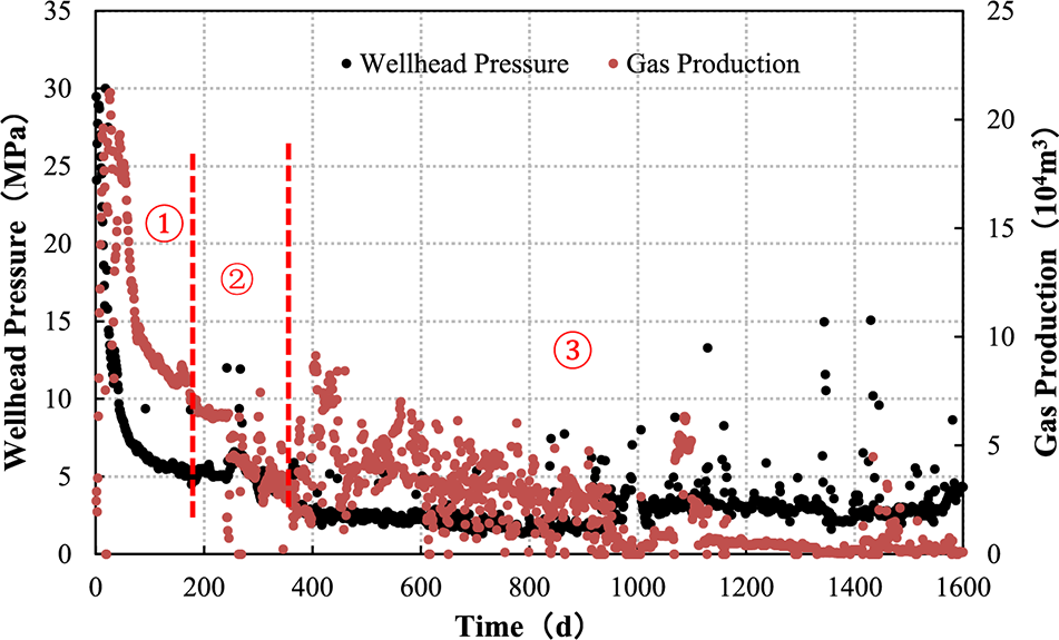
Figure 1: Schematic diagram of production stage division of shale gas well

Judging from the actual production in the field, there are great differences in the duration of each stage. In the early stage of shale gas development, the production time of casing was long, generally more than 600 days, and even as long as 1200 days for some gas wells. With the gradual maturity of drainage and gas production technology, the timing of tubing intervention has been advanced. The duration of casing production has been shortened, and mainly takes 180 days or less at present. At the same time, due to the scale of hydraulic fracturing, reservoir flow capacity, organic matter content and other factors, the duration of each production well in the stages of casing production and tubing production varies greatly, thus affecting the time of occurrence of the low-pressure and low-production stage. However, in general, the pressure and production of shale gas wells decrease rapidly, the low-pressure and low-production stage lasts longer, and the cumulative gas production in this stage accounts for a large proportion. Shale gas wells have great gas production potential under low pressure.

Due to the special extraction methods, the first few months of shale gas well production is the main period of fracturing-fluid flowback. During this period, the daily water production rises to peak levels and then drops rapidly. It generally decreases to a lower level after 40~90 days in shallow shale gas wells (buried below 3,500 m in depth). In contrast, after 90 days, the daily water production is still at a high level in the production of deep shale gas wells (buried over 3,500 m deep). It is relatively large in the middle and later stages of production. However, the WGR variation of both shallow and deep shale gas wells basically meets the power function relationship, as shown in Fig. 2.

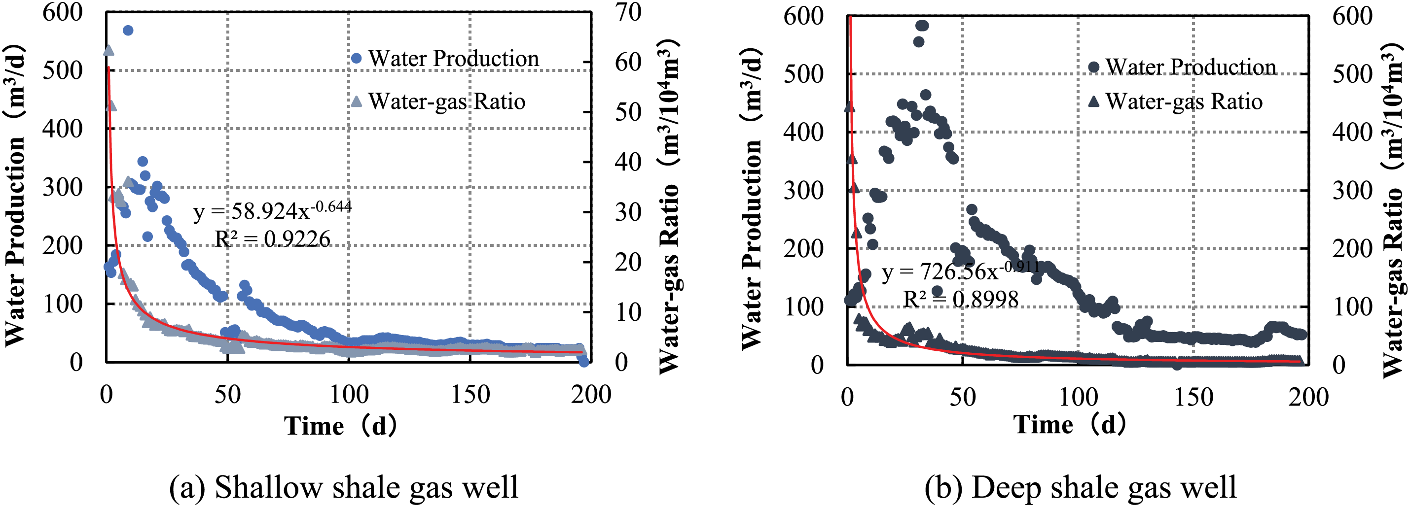
Figure 2: Variation curve of daily water production and WGR in different shale gas wells

2.2 Computational Models and Conditions

Based on the production characteristics of shale gas, a numerical simulation method was used to preliminarily explore the influence of different well types on gas-liquid two-phase distribution when tubing was running at 60°.

Shale gas wells can be classified into three types: up-dip, down-dip, and nearly horizontal. Its horizontal section is long, up to 3,000 m. And the dip angle of the horizontal section of most gas wells is within −10°~10°. Three simplified wellbore models of up-dip, horizontal, and down-dip wells were established according to the structural characteristics of shale gas wells (see Fig. 3). The models consist of vertical, inclined, and horizontal sections. Both the vertical and horizontal sections are round tubes with dimensions of Φ60 mm × 3,000 m and Ф140 mm × 3,000 m, respectively. An inclined section connects them with a radius of curvature of 1 m. The horizontal section of the up-dip and down-dip wells is inclined by 10°, and the difference lies in one up-dip and the other down-dip. Fig. 4 shows the definition of the tubing running depth (the tubing runs 20° in the example), which the inclined section composed of a 60° circular pipe (Φ60 mm) and a 30° circular tube (Φ140 mm).

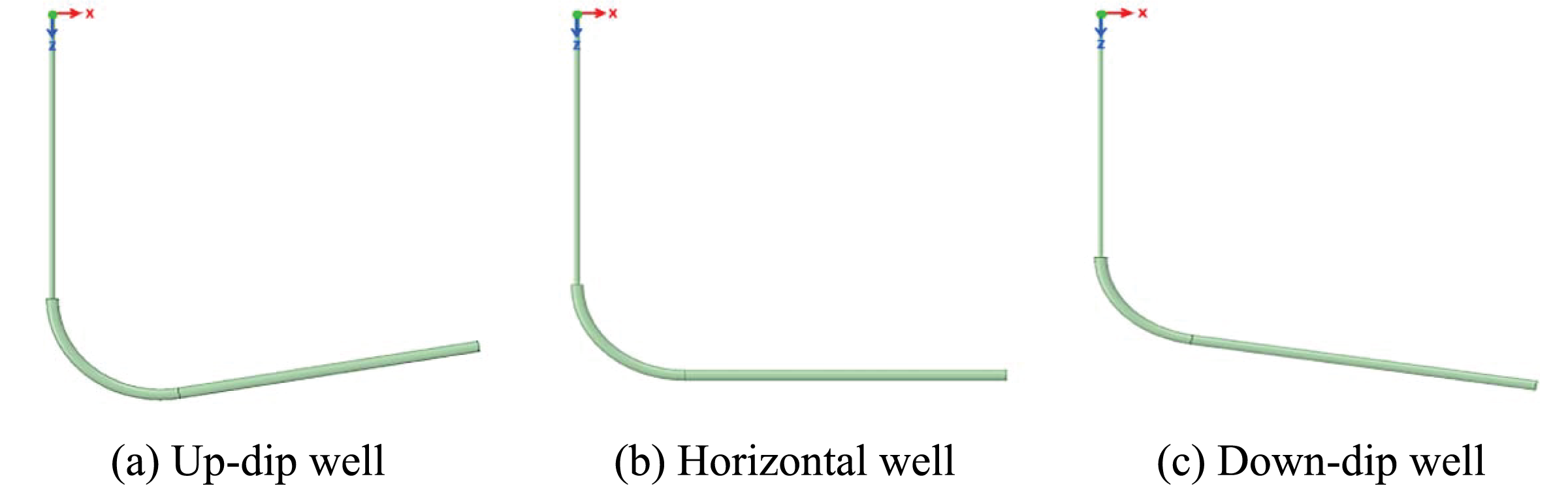
Figure 3: Simplified wellbore models for up-dip, horizontal and down-dip wells

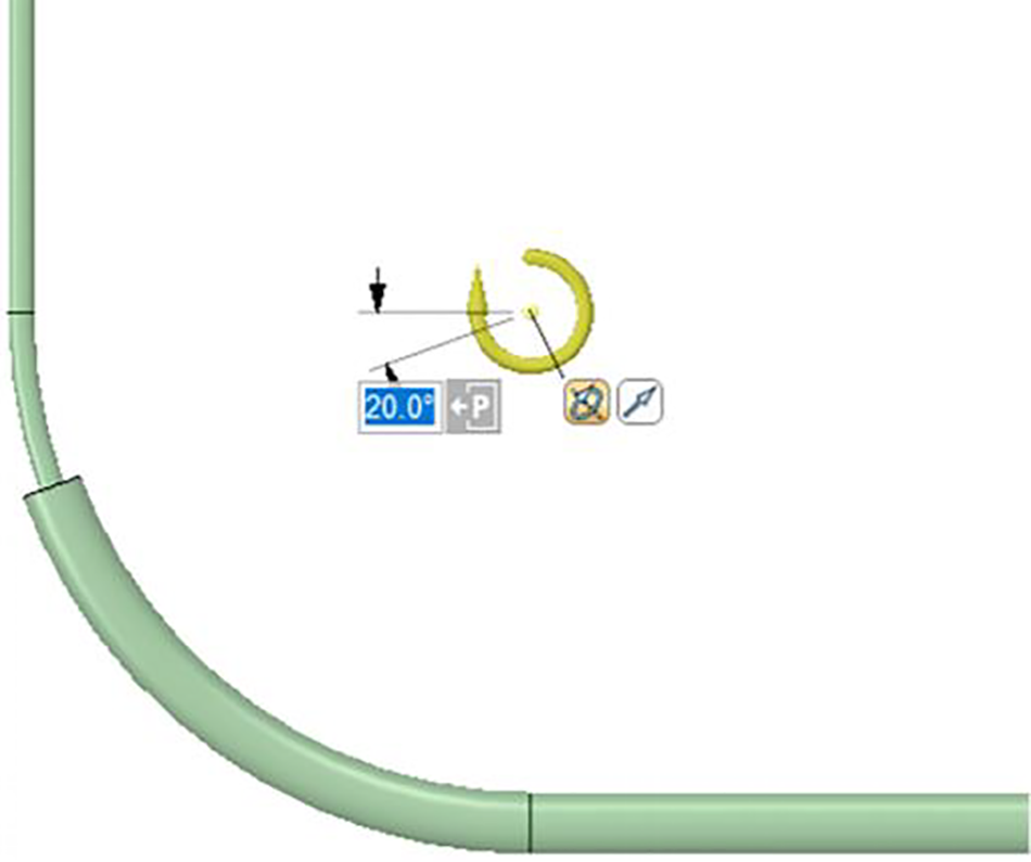
Figure 4: The definition of tubing running depth (20° example)

The fluid domain mesh was divided by a curvature-based encryption method, and the boundary mesh was set on the wall (10 layers were divided by the smooth transition method). The total number of grid cells was about 380,000, as shown in Fig. 5. The mesh quality was evaluated by the orthogonality standard. The orthogonality of most meshes was greater than 0.4, indicating that the overall mesh quality was good. The minimum orthogonality in the region was 0.11, which met the calculation requirements.

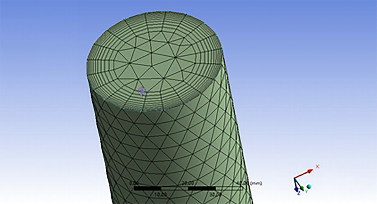
Figure 5: The grid distribution

Computational Fluid Dynamics (CFD) was used to study the fluid distribution characteristics in the wellbore. The flow is approximated as a steady-state flow and calculated using a pressure-based N-S equation solver [15]. During the simulation, the different gas-liquid two-phase fluids in the wellbore were set as methane and liquid water. The Mixture multiphase flow and Realizable k-ε turbulence models [16] were used to simulate the interaction between mixed fluids. The calculation area was discretized based on the finite element volume method, and the second-order upwind scheme was used to ensure the calculation accuracy. And the SIMPLE algorithm was used to carry out the flow field coupling [17].

2.3 Pipe Flow Models

The existing multiphase pipe flow models usually include four categories, namely homogeneous flow, split-phase flow (drift flow), split-flow and combined models. Homogeneous flow model is used to calculate gas-liquid two-phase flow as a single-phase flow without considering the interaction between gas and liquid, which is suitable for dispersible bubble flow. The split-phase flow (drift flow) model regards gas and liquid as two completely separated fluids but does not consider the interaction between the two phases. Therefore, it is suitable for stratified and annular flows, and the typical models are Lockhart & Martinelli [18] and Hubbard & Dukler models [19]. The split-flow model is a calculation formula derived by analyzing different flow patterns to clarify the gas-liquid two-phase flow pattern. Therefore, the calculation formula of pipe flow is also different for different flow patterns, such as Baker, Mukherjee & Brill and Beggs & Brill models [20–22]. Different formulas are used to calculate the pressure drop generated by friction, elevation, and acceleration, then combined to form a pipe flow calculation formula with higher accuracy, resulting in the combined model.

Pipe flow models widely used in engineering are generally empirical relations, mainly including Hagedorn & Brown, Duns & Ros, Beggs & Brill, Hagedorn & Brown Revised, Govier, Aziz & Fogarasi, Beggs & Brill Revised, Mukherjee & Brill, Orkiszewski and Gray [23–25]. The characteristics of common pipe flow models are presented in Table 1.

3  Results and Discussion

3.1 Analysis of Gas-Liquid Distribution Characteristics

Considering that the shale gas well has been in the stage of low-pressure and low-production for a long time, the calculation parameters of each model were kept unchanged during the simulation. And the WGR was set at 2.5 m3/104m3, in which the gas injection volume was 2 × 104 m3/d, and the liquid injection volume was 5 m3/d. The calculated results are shown in Figs. 6–8.

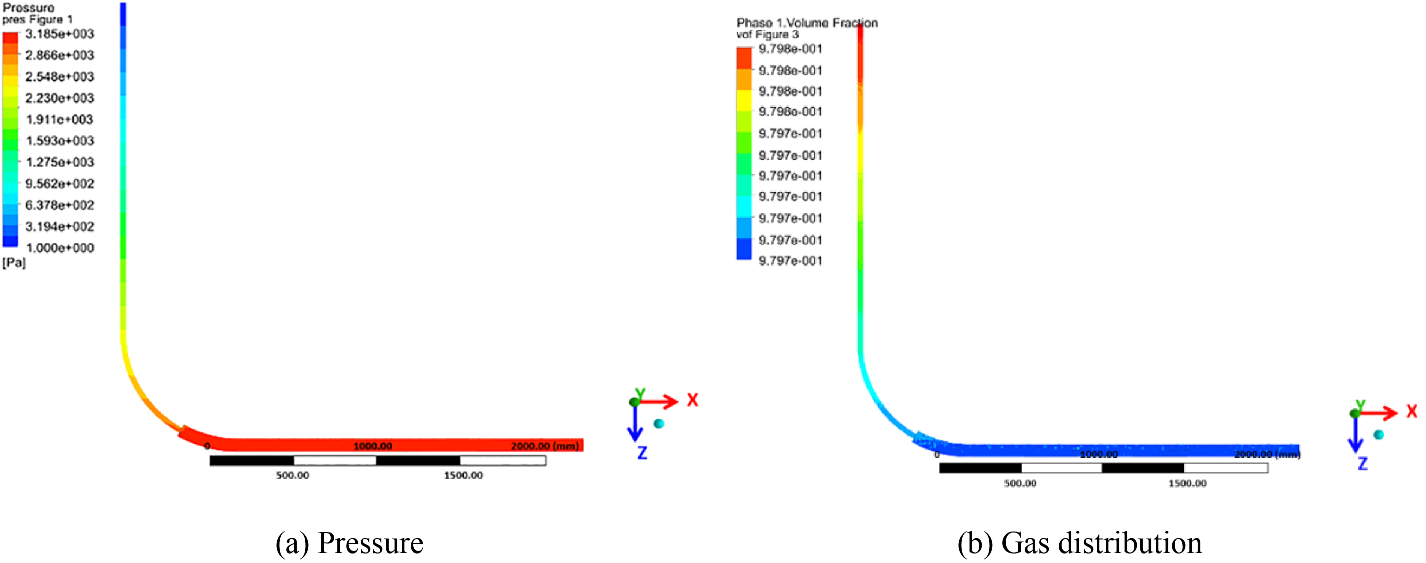
Figure 6: The cloud maps of pressure and gas distribution in horizontal well

Figure 7: The cloud maps of pressure and gas distribution in up-dip well

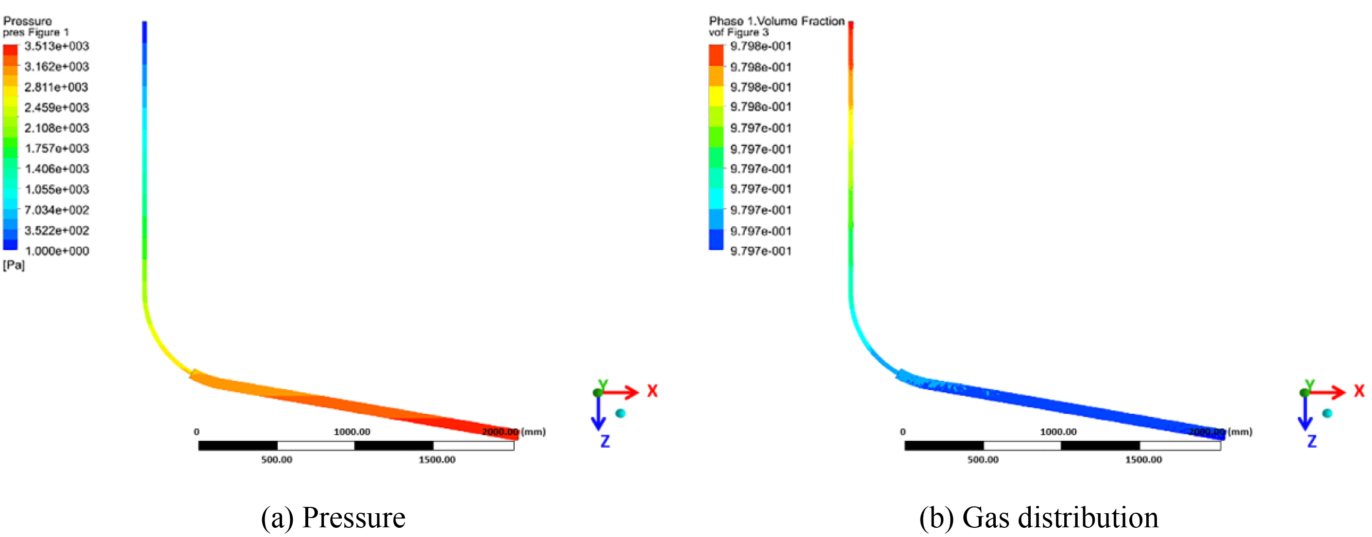
Figure 8: The cloud maps of pressure and gas distribution in down-dip well

As shown in the pressure and gas distribution diagrams of different types of gas wells, the liquid distribution is relatively uniform due to the slight pressure loss in the horizontal section of the horizontal well. Because of fluid slippage in the deviated section, pressure loss increases, and the liquid phase gradually accumulates in the horizontal section under the influence of gravity. The gas accumulates at the toe of the up-dip well and the pressure increases gradually, driving the liquid out of the wellbore. However, liquid slippage in the deviated section leads to increased pressure loss and easy accumulation of liquid phase. In the down-dip well, the liquid drops from the deviated section to the horizontal section, where the pressure loss is the greatest and the liquid phase accumulates from the toe of the horizontal section. Previous research results show that the gas-liquid two-phase flow also has a similar distribution law when flowing in a single pipe diameter [30–32], indicating the effect of running tubing on gas-liquid distribution in the wellbore is not significant, and the well structure is the main factor. Therefore, it is necessary to work on the gas-liquid distribution characteristics of different gas wells to effectively solve the poor liquid-carrying capacity when further exploring the reasonable tubing running depth or designing artificial lift.

3.2 Optimization of Pipe Flow Model

Shale gas well actually has a “spoon-shaped” wellbore trajectory, and its horizontal section is not absolutely linear but wavy. As a result, the wellbore flow of shale gas wells is very complicated. However, conventional pipe flow models vary in adaptability. We must evaluate and select suitable models to accurately calculate wellbore pressure and lay a solid foundation for process design.

In the evaluation process, the pressure profiles of two different gas wells were calculated using multiple models, and the adaptability of each model was preliminarily understood. Then, a large amount of data was used to analyze the model to comprehensively find universal rules. Finally, the optimal model was selected by refining the analysis area and using the calculation error.

3.2.1 Evaluation of the Model

The afore-mentioned nine gas-liquid two-phase flow models were fitted and evaluated by using 97 groups of measured flow pressure data of shale gas wells. During the process of fitting, it was found that the calculation accuracy of each pipe flow model was different in variable WGR.

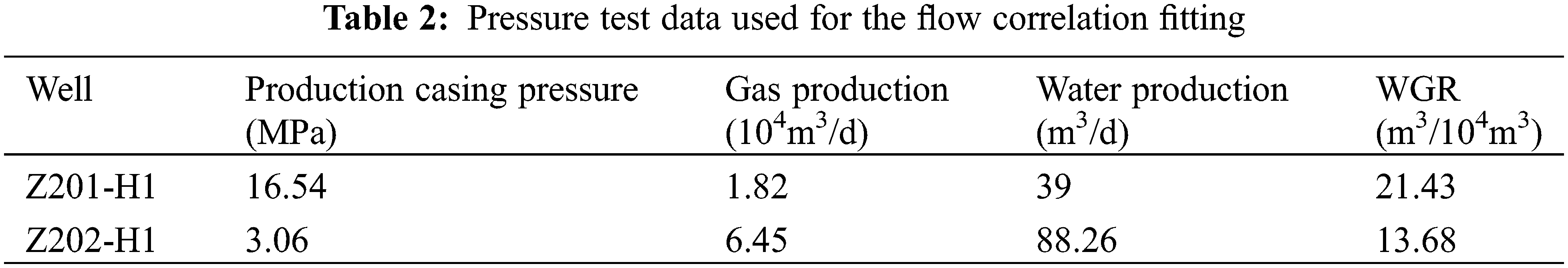
Figs. 9 and 10 show the results of fitting of nine models with pressure measurements from two shale gas wells. For well Z201-H1, the calculated results of all models are generally small, and the consequences of the Gray model are close to the measured pressure. However, for well Z202-H1, the computed results of the Hagedorn & Brown Revised (HBR) model are close to the measured pressure. At the same time, the Gray model values are generally large, and the other seven models’ values are too small as a whole. The test data of the two wells are presented in Table 2.

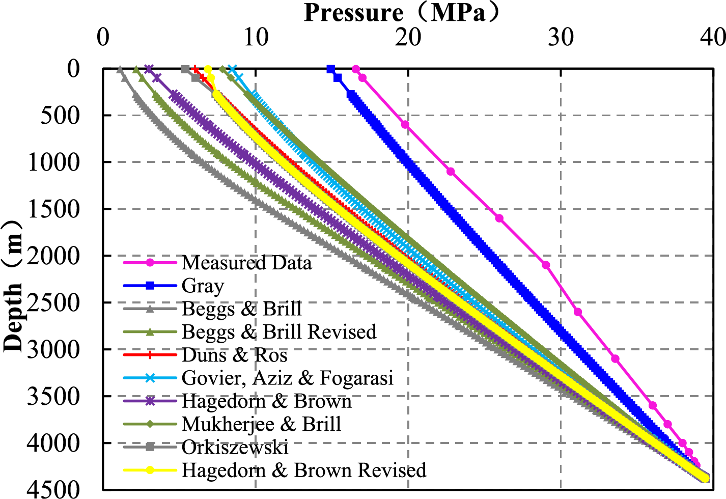
Figure 9: The diagram of the fitting of wellbore pressure profile in well Z201-H1

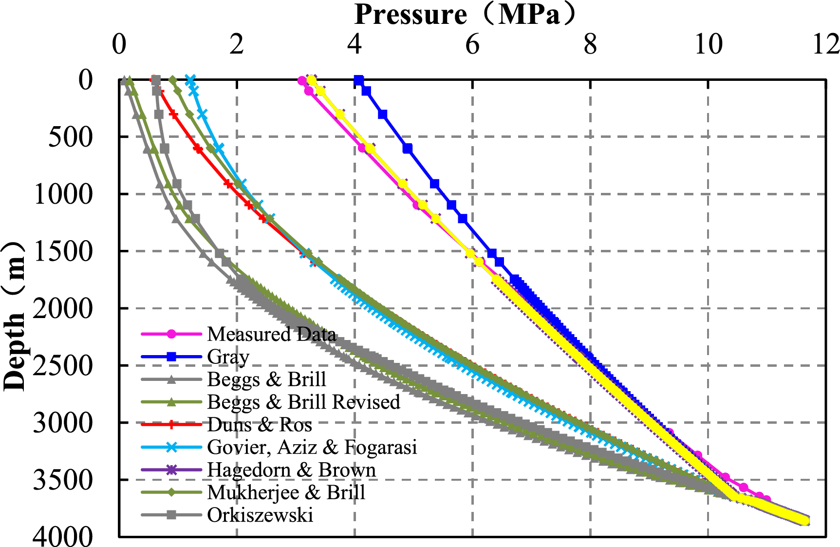
Figure 10: The diagram of the fitting of wellbore pressure profile in well Z202-H1

Based on the calculated results form the two wells, 97 pressure measurement data of shale gas wells were sorted out to evaluate the calculation accuracy of nine pipe flow models under different WGR. Basic information of shale gas wells: the vertical depth is 2200~4400 m, the well type is a horizontal well, and the gas production is 0.23~22.56 × 104 m3/d, WGR 0.11~29.82 m3/104m3, wellhead pressure 3.11~21.08 MPa, measured bottom-hole flow pressure 4.59~45.03 MPa. The results of the comparison between the actual pressure and the wellhead pressure calculated by nine models are shown in Fig. 11.

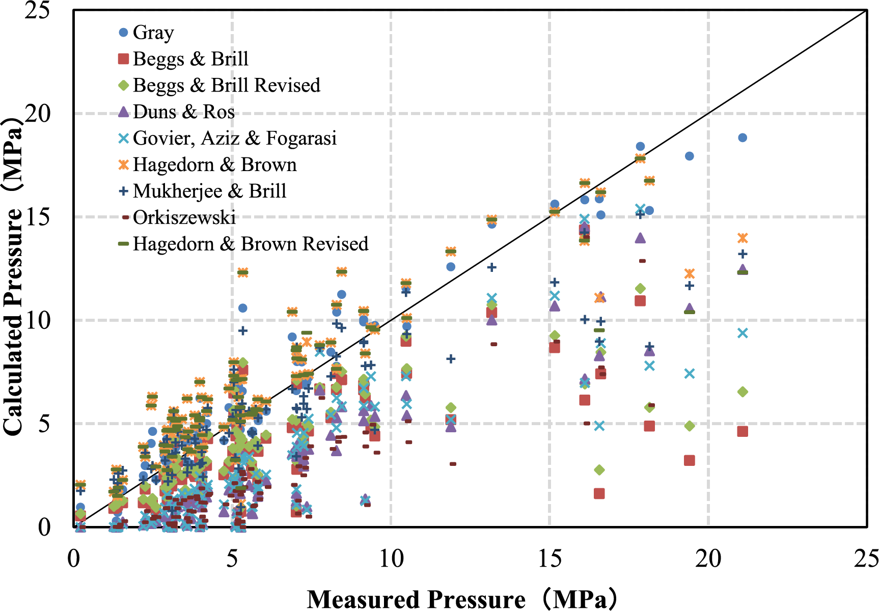
Figure 11: Comparison of wellhead pressure calculated by different models with measured values

As evident from Fig. 10, the Gray, Beggs & Brill Revised (BBR), Mukherjee & Brill (MB), Hagedorn & Brown (HB), and HBR models, all have relatively high calculation accuracy. On the other hand, the calculated results of the remaining 4 models are generally small.

The relative errors calculated by the nine models show that the error changes significantly when the WGR is around 0.8, 8.5, 20.0 m3/104m3 (see Fig. 12). By analysis, the models with high calculation accuracy in different WGR ranges are:

1.    When the WGR is less than 0.8 m3/104m3, the average relative error of the BBR model is 13.11%, and the accuracy is the highest.

2.    When the WGR is 0.8~8.5 m3/104m3, the average relative error of the Gray model is 7.79%, and the accuracy is the highest, followed by the HB or HBR model, with an average relative error of 11.82%.

3.    When the WGR is 8.5~20.0 m3/104m3, the average relative error of the HB or HBR model is 16.93%, and the accuracy is the highest.

4.    When the WGR is greater than 20.0 m3/104m3, the average relative error of the Gray model is 7.9%, and the accuracy is the highest.

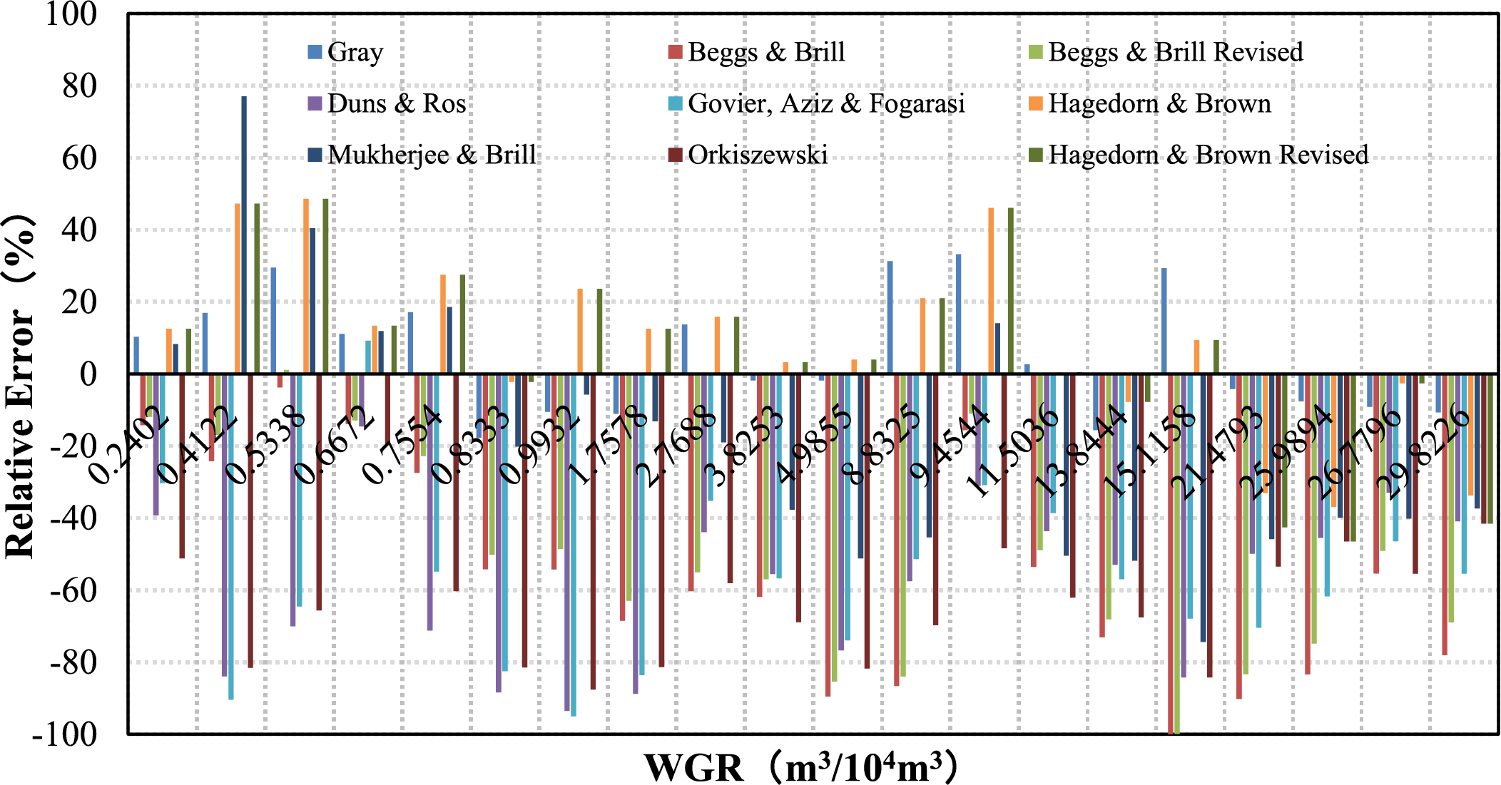
Figure 12: Distribution of relative error of nine models under different WGR

3.2.2 Selection of the Optimum Model

To select the pipe flow model that meets the actual conditions of shale gas wells, the range of WGR was divided into 5 intervals, and the average relative errors calculated by 9 models were compared and analyzed. The results are presented in Table 3.

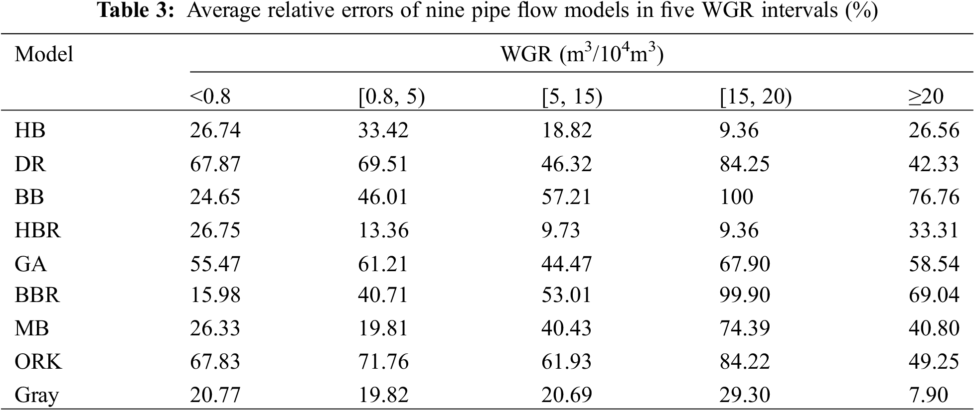
According to the comparison of relative errors, it is recommended to use different pipe flow models in different WGR ranges. The BBR model is adopted when the WGR is less than 0.8 m3/104m3; the HBR model is adopted when the WGR is between 0.8~20.0 m3/104m3; and when the WGR is greater than 20.0 m3/104m3, the Gray model is adopted.

Combined with the variation law of WGR in shale gas wells, it is considered that the Gray model should be used to predict the wellbore pressure distribution in the early stage of casing production, and the HBR model should be used in the middle and later stages of casing production. The HBR model is mainly used in the production stage of tubing.

3.2.3 Application

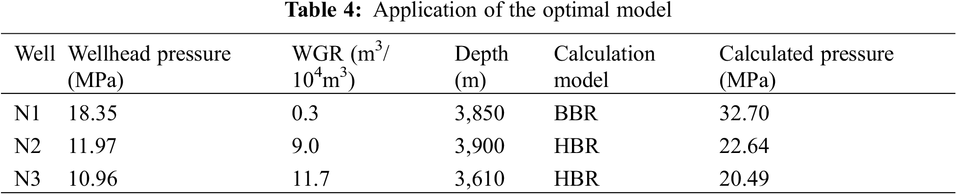
Three gas wells with different production conditions were randomly selected as an example calculation. The appropriate pipe flow model was selected according to the WGR to calculate the bottom hole pressure. Table 4 presents the calculated flow pressure at the target position of each well, which provides a basis for the design of gas production process.

These models are covered by most professional analysis software and are highly maneuverable. But the research results only apply to shale gas wells, not wellbore flow in other gas reservoirs. Furthermore, the statistical law of wellbore two-phase flow may change with the increase of shale gas wells.

4  Conclusions

In this study, different analyses were performed to evaluate and compare the performance of gas-liquid two-phase flow in shale gas horizontal wells. Based on these analyses, it can be concluded that the production of shale gas wells decreases rapidly, and the “spoon-shaped” hole is an important factor affecting the gas-liquid two-phase flow in the wellbore. The adaptability of common pipe flow models is different, and their accuracy was evaluated by using 97 sets of measured flow pressure data. The BBR, HBR and Gray models are three models with high precision, respectively used under different WGR ranges.

It is proved again by numerical simulation that the deviated section is the most difficult section to carry fluid. However, due to the influence of well type, the accumulation characteristics of liquid phase in up-dip, horizontal and down-dip wells are different, resulting in different wellbore pressure drop. The WGR represents the dynamic change of two-phase flow. Obviously, it can be used as a technical boundary to effectively select a representative model from multiple models.

The BBR model gives good results if used with a WGR of less than 0.8 m3/104m3. However, it should be used with caution because its calculation error may be large. The Gray model on the other hand, can give a good match on wells with WGR greater than 20.0 m3/104m3. The HBR model can be used in the remaining cases.

In conclusion, it should be noted that the law of gas-liquid two-phase flow in shale gas wells is particularly complex. The evaluation of wellbore pipe flow model has laid a solid foundation for the accuracy of wellbore fluid pressure distribution prediction and the rationality of process design.

Acknowledgement: This study would not have materialized but for the numerous support and encouragement we have received from many parties. The authors would like to take this opportunity to express our heartfelt gratitude to all who have assisted us.

Funding Statement: This work was supported by the company’s scientific research project “Study on Prediction Method of Liquid Carrying Capacity of Shale Gas Well with High Liquid-Gas Ratio” (Project No. 20220303-05).

Conflicts of Interest: The authors declare that they have no conflicts of interest to report regarding the present study.

References

1. Williams, A. (2009). Predicting two-phase flow regimes in segments of a gas/condensate well. SPE Annual Technical Conference and Exhibition, pp. 1–12. Louisiana, New Orleans. [Google Scholar]

2. Lina, M. T., Jhara, O. P., Paula, P., Juan Pablo, V., Deisy, B. et al. (2020). Comparison of 63 different void fraction correlations for different flow patterns, pipe inclinations, and liquid viscosities. SN Applied Sciences, 2(10), 1695.1–1695.24. [Google Scholar]

3. Mansour, M. H., Zahran, A. A., Rabie, L. H., Shabaka, I. M. (2021). Experimental and numerical study of air-water flow characteristics in a horizontal duct. Proceedings of the Institution of Mechanical Engineers, Part C: Journal of Mechanical Engineering Science, 235(5), 843–858. [Google Scholar]

4. Kim, T. W., Woo, N. S., Han, S. M., Kim, Y. J. (2020). Optimization and extended applicability of simplified slug flow model for liquid-gas flow in horizontal and near horizontal pipes. Energies, 13(4), 842. [Google Scholar]

5. Waltrich, P. J., Barbosa, J. R. (2011). Performance of vertical transient two-phase flow models applied to liquid loading in gas wells. SPE Annual Technical Conference and Exhibition, pp. 1–15. Colorado, USA. [Google Scholar]

6. Hategan, F., Hawkes, R. (2012). Well production performance analysis for unconventional shale gas reservoirs. SPE Canadian Unconventional Resources Conference, pp. 1–20. Alberta, Canada. [Google Scholar]

7. Williams-Kovacs, J. D., Clarkson, C. R. (2015). A modified approach for modelling 2-phase flowback from multi-fractured horizontal shale gas wells. Unconventional Resources Technology Conference, pp. 1–11. San Antonio, USA. [Google Scholar]

8. Uzun, I., Assiri, W., Eker, E. (2019). Application of well interference test using distributed pressure sensors to optimize well spacing in unconventional shale reservoirs. Abu Dhabi International Petroleum Exhibition & Conference, pp. 1–13. Abu Dhabi, United Arab Emirates. [Google Scholar]

9. Li, M. (2021). Study on wellbore flow simulation and liquid carrying model of shale gas well. Journal of Jianghan Petroleum University of Staff and Workers, 34(4), 27–29. [Google Scholar]

10. He, Y. Q., Chen, Q., Wu, T. T., Zeng, L. J., Wang, Y. T. et al. (2022). Research on the flow law of shale gas in horizontal wellbore: Taking C01 well area as an example. Chemical Industry of Oil & Gas, 51(2), 77–82. [Google Scholar]

11. Yu, F., Chen, J. X., Ye, C. Q., Xiang, J. H., Yang, Z. et al. (2022). Horizontal-well plunger technology and its application to shale gas, Changning block, Sichuan Basin. Natural Gas Exploration and Development, 45(1), 105–110. [Google Scholar]

12. Liu, H., Qin, W., Hu, C. Q., Song, W., Zhu, Y. J. et al. (2021). Prediction of gas-liquid two-phase flow regime in the wellbore of 202H shale gas well. Journal of Chongqing University of Science and Technology (Natural Science), 23(5), 20–25. [Google Scholar]

13. Liu, Y. H. (2019). Study on drainage and production technology of Changning shale gas horizontal wells (Master Thesis). Southwest Petroleum University, Chengdu, China. [Google Scholar]

14. Xie, N. X., Cai, D. G., Ye, C. Q., Tang, H. B., Wang, Q. R. et al. (2022). New production pressure drop calculation model for shale gas horizontal well. Drilling & Production Technology, 45(1), 75–80. [Google Scholar]

15. Watterson, J. K. (1994). A pressure-based flow solver for the 3D Navier-Stokes equations on unstructured and adaptive meshes. Fluid Dynamics Conference, pp. 1–12. Colorado Springs, USA. [Google Scholar]

16. Li, C., Ji, S. M., Tan, D. P. (2012). Softness abrasive flow method oriented to tiny scale mold structural surface. The International Journal of Advanced Manufacturing Technology, 61(9-12), 975–987. [Google Scholar]

17. Anderson, J. D. (2007). Computational fluid dynamics. China: Machinery Industry Press. [Google Scholar]

18. Lockhart, R. W., Martinelli, R. C. (1949). Proposed correlation of data for isothermal two-phase, two-component flow in pipes. Chemical Engineering Progress, 45(1), 39–48. [Google Scholar]

19. Hubbard, M. G., Dukler, A. E. (1966). The characterization of flow regimes for horizontal two-phase flow. In: Heat transfer and fluid mechanics institute, pp. 100–121. USA: Academic Press. [Google Scholar]

20. Baker, O. (1954). Simultaneous flow of oil and gas. Oil and Gas Journal, 53, 185–195. [Google Scholar]

21. Mukherjee, H., Brill, J. P. (1983). Liquid holdup correlations for inclined two-phase flow. Journal of Petroleum Technology, 35(5), 1003–1008. [Google Scholar]

22. Beggs, D. H., Brill, J. P. (1973). A study of two-phase flow in inclined pipes. JPT, 25(5), 607–617. [Google Scholar]

23. Zhong, H. Q., Li, Y. C., Liu, Y. H., Li, C. J., Li, W. (2008). BP neural network-based selection of the optimum model of multiphase flow in pipes and its application. Sciencepaper Online, 3(11), 873–878. [Google Scholar]

24. He, H. Q., Ming, R. Q., Rui, Q. Y., Lei, M., Cao, G. Q. (2018). Evaluation and optimization of two-phase flow pressure drop model for continuous pipe drainage gas production well. China Petroleum Machinery, 46(10), 49–54. [Google Scholar]

25. Chen, D. C., Xu, Y. X., Meng, H. X., Peng, G. Q., Zhou, Z. F. (2017). Evaluation and optimization of pressure drop calculation model for gas-liquid two-phase pipe flow in gas well. Fault Block Oil and Gas Field, 24(6), 840–843. [Google Scholar]

26. Ju, Y. J., Liu, X. G., Gao, Y. L., Zeng, N., Wang, P. (2008). Review of friction calculation methods for multiphase pipe flow. China Petroleum and Chemical Industry, 26(10), 55–58. [Google Scholar]

27. Zhang, G. D., Shi, G. Y., Wang, D. B., Chen, G. (2019). Selection and adaptability analysis of “flow correlation” of multiphase flow model. Petroleum Planning and Design, 30(5), 9–12. [Google Scholar]

28. He, Z. P. (2017). Study on the influence of pipe diameter on flow pattern and pressure drop in gas-water two-phase ascending pipe (Master Thesis). Southwest Petroleum University, Chengdu, China. [Google Scholar]

29. Yan, H., Shang, S. F., Wang, H., Li, M. L., Zhong, H. Q. et al. (2020). A new method for the analysis of liquid-loading capacity of shale gas well. Natural Gas Exploration and Development, 43(2), 110–115. [Google Scholar]

30. Liu, B. (2015). Prediction model and application of fluid loading in horizontal well in low permeability gas reservoirs controlled by well trajectory (Master Thesis). Southwest Petroleum University, Chengdu, China. [Google Scholar]

31. Dai, L. Z., Cai, L., Zhang, X. K., Ji, G. F., Qu, D. X. (2019). Numerical simulation of fluid loading in small-angle undulating pipe sections in horizontal well. Fault Block Oil and Gas Field, 26(6), 747–750. [Google Scholar]

32. Zhou, X. F., Zou, Y. F., Fu, C. M., Yang, G. T., Liu, Y. H. (2012). Influence of horizontal well trajectory on drainage and gas production. Complex Oil and Gas Reservoir, 5(1), 4. [Google Scholar]