Numerical Analysis of Flow-Induced Vibration and Noise Generation in a Variable Cross-Section Channel

1  Introduction

The flow channel with variable cross-section serves as the variation for the velocity and pressure of the fluid [1]. When the fluid passes through the variable cross-section area, strong vibration and noise will be generated, which will deteriorate the stability of industrial equipment, the safety of buildings, and the concealment of ships. Therefore, it is necessary to research the vibration and noise characteristics of flow channels with variable cross-section considering the fluid-solid interaction.

In recent years, more and more researchers carried out theoretical analyses [2–4], experimental researches [5–8], and numerical simulations [9–13] on the generation mechanism of flow channel noise and vibration. Liu et al. [14] proposed a transfer matrix method in the frequency domain considering fluid-structure interaction of liquid-filled flow channel with elastic constraints, which can easily analyze all the classical constraints. Li et al. [15] proposed an implicit Immersed Boundary method (IBM) combined with Lattice Boltzmann method (LBM), and Finite Element method (FEM), which is an efficient and reliable fluid-structure interaction numerical simulation method. Han et al. [16] developed a pressure-based method for estimating the sound power radiated from a flow duct wall. Liu et al. [17] used the LES method and FW-H acoustic analogy theory to numerically simulate the elbow pipe, and found that elbow noise is broadband noise. Han et al. [18] researched the noise of natural gas manifold through numerical simulations and experiments, and obtained the best cross-sectional area ratio of distribution pipe to inlet and outlet flow channel. Hambric et al. [19] used the method of interaction CFD and structural acoustic model to calculate the structure- and fluid-borne vibro-acoustic power spectra of a continuous 90° piping elbow. Mori et al. [20] conducted experiments and simulations to research the acoustic and vibration characteristics of tee with square cross-section, and the results showed that the sound produced does not depend on the inflow velocity, but on the acoustic frequency characteristics of the tee. Zhao et al. [21] researched the influence of the transition form on the acoustic characteristics of the flow channel with variable cross-section. The results showed that the flow-induced noise in the flow channel with variable cross-section increase with the increase of the flow velocity, and the noise of the tapered flow channel is significantly less than that of the suddenly-contracted flow channel.

However, there are few researchers on the noise of the flow channel with variable cross-section, and the present studies are limited to flow-induced noise. In this paper, finite element method and modal analysis theory are used to analyze the vibration and noise characteristics considering fluid-structure interaction. The changing laws of excitation force, flow-induced noise, and structure-borne noise at different flow velocities are researched. This paper can provide guidance for the cooperative research of structural optimization and noise control for the flow channel with variable cross-section.

2  Methodology

2.1 Mathematical Model

In this section, mathematical models are introduced. First, the steady-state flow field in the flow channel is calculated. The obtained steady-state flow field is used as the initial flow field for transient flow field calculation and aerodynamic noise calculation based on the acoustic analogy method. After that, the modal calculation of the flow channel is carried out with the collected pressure pulsation characteristics of the flow channel wall as the load of the flow channel wall, so as to obtain the modal mode shape and structure noise of the flow channel.

2.1.1 Flow Field Computational Model

In the numerical simulation calculation of the flow field, the fluid inside the flow channel is water, and the fluid outside the flow channel is air. Both of these two fluids satisfy the mass conservation equation, momentum conservation equation and energy conservation equation.

(1) mass conservation equation:

∂ρ∂t+∂(ρu)∂x+∂(ρv)∂y+∂(ρw)∂z=0 (1)

where ρ is the density of the fluid, kg/s; u, v, w are the partial velocities in the x, y, and z directions, respectively, m/s; t is the flow time, s.

In this paper, water and air can be regarded as incompressible fluids with constant density, so the equation can be simplified to:

∂u∂x+∂v∂y+∂w∂z=0 (2)

(2) momentum conservation equation:

∂u∂t+u∂u∂x+v∂u∂y+w∂u∂z=fx−1ρ∂p∂x+μ(∂2u∂x2+∂2u∂y2+∂2u∂z2) (3)

∂v∂t+u∂v∂x+v∂v∂y+w∂v∂z=fy−1ρ∂p∂y+μ(∂2v∂x2+∂2v∂y2+∂2v∂z2) (4)

∂w∂t+u∂w∂x+v∂w∂y+w∂w∂z=fz−1ρ∂p∂z+μ(∂2w∂x2+∂2w∂y2+∂2w∂z2) (5)

where fx, fy, fz are the micro-element volume forces in the x, y, and z directions, respectively, N; p is the pressure acting on the micro-element, Pa; μ is the kinematic viscosity of the fluid, m2/s.

(3) energy conservation equation:

∂(ρT)∂t+div(ρUT)=div(kcpgradT)+ST (6)

where T is the fluid temperature, K; cp is the specific heat capacity of the fluid, J/(kg·K) k is the heat transfer coefficient of the fluid, w/(m2·K); ST is the internal heat source of the fluid and the heat energy converted from viscous mechanical energy, J.

Since this paper explores the change of the internal flow field and noise distribution of the variable-section tube, the heat exchange between the fluid and the outside is not considered, so only the mass conservation equation and the momentum conservation equation are considered.

2.1.2 Flow-Induced Noise Computational Model

The flow-induced noise is mainly caused by the interaction between the fluid and the solid wall. Solid boundary generates a dipole source whose radiated noise power is proportional to the sixth power of the flow velocity. Ffowcs Williams-Hawkings (FW-H) acoustic analogy theory is developed from Lighthill acoustic analogy theory, which can accurately describe the sound between moving objects and fluid. FW-H acoustic analogy [22] is used to obtain the characteristics of the flow-induced noise [23,24]. The FW-H acoustic model can be derived by manipulating the continuity equation and the Navier-Stokes equations, and it is essentially an inhomogeneous wave equation.

FW-H acoustic equation is as follows:

1c02∂2p∂t2−∇2p′=∂2∂xi∂xj[TijH(f)]−∂∂xi[Pijnjδ(f)]+∂∂t[ρ0unδ(f)] (7)

where p is the far-field sound pressure, Pa; δ(f) is the Dikra function; H(f) is the Heaviside function; f is the wall function; vn is the normal velocity component of the control surface; and un is the fluid velocity at the control surface normal component; pij is the stress tensor; Tij is the Lighthill tensor.

2.1.3 Modal Analysis Theory

The mode shape is an inherent property of the flow channel, which indicates the vibration under excitation force. Modal analysis can be used to obtain the mode shapes after determining the geometric structure, material properties, and constraints. Modal analysis is of great significance to acoustic and vibration analysis of flow channels.

According to the theory of modal analysis, the equation of structural vibration is as follows:

MsU⋅⋅+GsU⋅+KsU=Fs (8)

where Ms is the mass matrix; Gs is the damping matrix; Ks is the stiffness; Fs is the excitation force vector; U⋅⋅ is the acceleration of the node in the structure, m/s2; U⋅ is the speed of the node, m/s; and U is the displacement vector of the node, m.

In the actual calculation, the vibration deformation of the structure is generally very small, so the influence of the damping term can be ignored. When analyzing the mode without external excitation force, the excitation force term is 0, which can be written as:

MsU⋅⋅+KsU=0 (9)

The solution can be written as:

U=U¯⋅sinω¯t (10)

where U¯ is the amplitude vector of the displacement vector U ; and ω¯ is the natural frequency of the structure, Hz.

Substituting Eq. (10) into Eq. (9):

(Ks−ω¯2Ms)U=0 (11)

Eq. (11) is the characteristic equation for solving the vibration of the flow channel with variable cross-section, and the characteristic roots ω¯i(i=1,2,⋅⋅⋅,n) and Ui(i=1,2,⋅⋅⋅,n) are the mode shapes at the natural frequency and the corresponding frequency under undamped conditions, respectively.

2.1.4 Vibroacoustic Computational Model

The theoretical basis of ANSYS acoustic finite element analysis is the sound field wave equation. The wave equation is mainly derived from the acoustic motion equation, the acoustic continuity equation, and the acoustic equation of state.

Acoustic motion equation:

∇p=−ρ0∂v∂x (12)

Acoustic continuity equation:

∂ρ∂t=−ρ0∇⋅v (13)

Acoustic equation of state:

∂p∂t=γpρ0∂ρ∂t (14)

The wave equation can be derived by combining the above three basic equations:

∂2p∂t2=c2∇2p (15)

where p is the pressure, Pa; ρ0 is the density of the medium under static state, kg/m3; v is the medium velocity, m/s; c is the propagation velocity of the sound wave in the fluid medium, m/s; γ is the ratio of the specific heat capacity at constant pressure to the specific heat capacity at constant volume.

2.1.5 Acoustic Source Intensity

In order to quantitatively study the characteristic distribution of the sound source in the flow channel with variable cross-section, this paper introduces the acoustic source intensity to analyze the generation mechanism and generation area of flow-induced noise, and its definition is as follows:

(1c02∂2∂t2−∇2)B=div(ω×v) (16)

S¯=1n∑i=1nSi (17)

ST=∑i=1n(Si−S¯)2n (18)

where the left side of Eq. (16) describes the propagation process of sound waves in the fluid, and the right side of the equation is the sound source term, and its value is the sound source value; B is the total entropy of the fluid, B=pρ+12v2 ; ω is the vorticity vector, ω=∇×v ; v is the velocity vector; Si is the sound source value at any point in the flow field at time i, kg·m3/s2; S¯ is the sound source average, kg·m3/s2; n is the number of iterations; ST is the acoustic source intensity.

2.2 Geometric Model and Numerical Method

This paper takes a Chinese national standard pipe with variable cross-section as the research object. As shown in Fig. 1, the wall thickness is 3 mm, the inlet inner diameter D is 50 mm, the outlet inner diameter d is 25 mm, the variable diameter angle is 15.2°, and the length of the inlet and outlet pipelines is 4D, 200 mm. The radial distance S between the sound pressure level receiver and the pipe is 1000 mm.

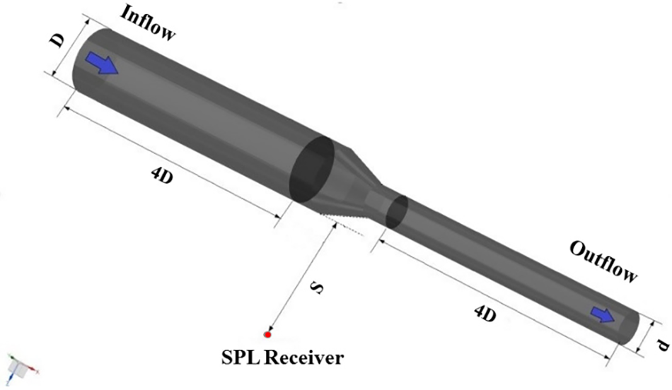
Figure 1: Geometric model and receiver

The material of the pipe is steel, the elastic modulus is 206 GPa, the Poisson ratio is 0.31, and the density is 7850 kg/m3. The working fluid in the flow channel is water, the density is 1000 kg/m3, the viscosity is 1.003 × 10−3 kg/(m∙s), and the sound velocity is 1425.7 m/s. The medium outside the flow channel is air, the density is 1.225 kg/m3 and the sound velocity is 340 m/s. The reference sound pressure in the acoustic calculations in this paper is all 2 × 10−5 Pa.

Steady-state simulations are performed using standard k-epsilon turbulence model and then used as initial conditions of transient simulations. The inlet boundary is set as the velocity-inlet, the outlet boundary is set as the outflow, and no-slip condition is applied on the wall. Transient flow fields are calculated using large eddy simulation (LES) with wall-adapting local eddy-viscosity (WALE) subgrid-scale model [25–28] by commercial CFD code ANSYS Fluent. The fluid studied in this paper is simplified to incompressible. The flow velocities are 1, 2, 3 m/s, and the corresponding Reynolds numbers are 55,693, 111,386, and 167,079, respectively. Time step is set to 10−5 s, and over 10,000 steps are taken to compute the turbulent flow.

The acoustic calculation domain created in this article consists of an air domain and a perfect matched layer. A cube domain with a side length of 1.5 m is established as the air domain outside the flow channel. In order to perform non-reflective treatment on all boundary surfaces of the acoustic envelope grid, a 20 mm thick perfect matched layer (PML) wrapped outside the air domain is built. The sound pressure on the outer surface of the PML is set to 0 to simulate the propagation of sound waves in an infinite domain.

The formula for the thickness of the PML layer is as follows:

δPML=c4fmax (19)

where δPML is the thickness of perfect matched layer, m; c is the velocity of sound propagation in the medium, m/s; and fmax is the maximum frequency, Hz.

The material medium in the acoustic grid is air. In order to ensure the accuracy of the acoustic calculation results, the minimum cell size of the acoustic grid should be less than one-sixth of the wavelength corresponding to the maximum frequency, the formula is as follows:

LS≤c6fmax (20)

where Ls is the length of the grid cell, m; c is the velocity of sound propagation in the medium, m/s; and fmax is the maximum frequency, Hz.

Then, a mapping relationship between the acoustic grid and the structured grid is established. A coupling interface is set between the acoustic grid and the structured grid to transmit pressure fluctuations and feedback calculations. Thus, the acoustic grid and the structural grid constitute an acoustic envelope grid as shown in Fig. 2.

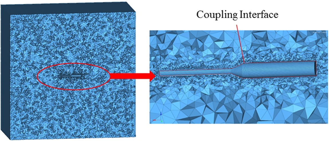
Figure 2: Acoustic envelope grid

2.3 Grid Refinement Study

The numerical simulation in this paper involves the fluid domain and the acoustic domain, and grids are established respectively for them. A hexahedral structured grid is used in computing the fluid domain. The boundary layer grid is encrypted so that the height of the first layer grid is 9.6 × 10−5 m, and the wall y+ is about 30. The grid independence of fluid domain has been verified. Table 1 shows the overall sound pressure level (OASPL) of the grids with different grid numbers. The relative deviation of grid-3 and grid-4 calculation results is 0.84%. It shows that when the number of grids is greater than 5.1 × 105, the grids are sufficient for numerical simulation. The relative deviation is calculated as Eq. (21).

Rn=SPLn−SPLn−1SPLn−1 (21)

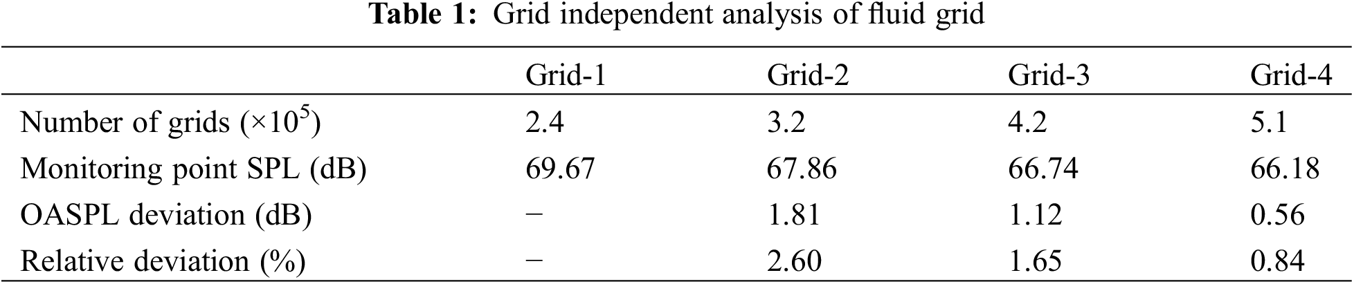
where Rn is the relative deviation; SPLn is the sound pressure level of the current grid; SPLn-1 is the sound pressure level of the previous grid.

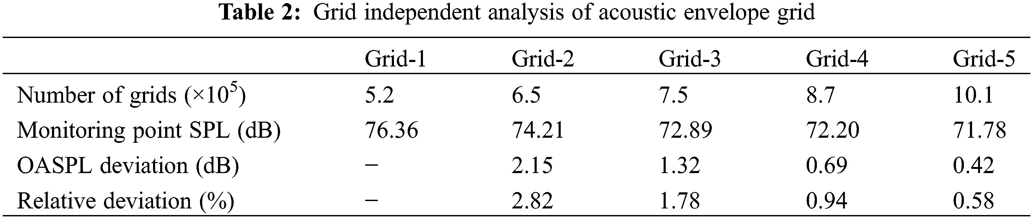
The independent analysis method of acoustic envelope grid is the same as that of fluid grid. Grid independent analysis is shown in the Table 2. The relative deviation of grid-3 and grid-4 calculation results is 0.94%. Both grid-4 and grid-5 can be used in numerical simulation. All simulations in this article are carried out using grid-4 to ensure the accuracy and efficiency of the calculation.

2.4 Validation

The accuracy of the model is verified by comparing with the experimental results. The calculation results are compared with the experimental results of flow-induced noise in the reference [29], and the accuracy of the numerical simulation method is verified. The pipe with variable cross-section used for verification is shown in Fig. 3. In the verification model, the material of the pipe is steel, the work fluid is air, the Reynolds number is 227907, and two receivers are set outside the pipe to monitor sound pressure level (SPL).

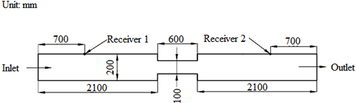
Figure 3: Validation model

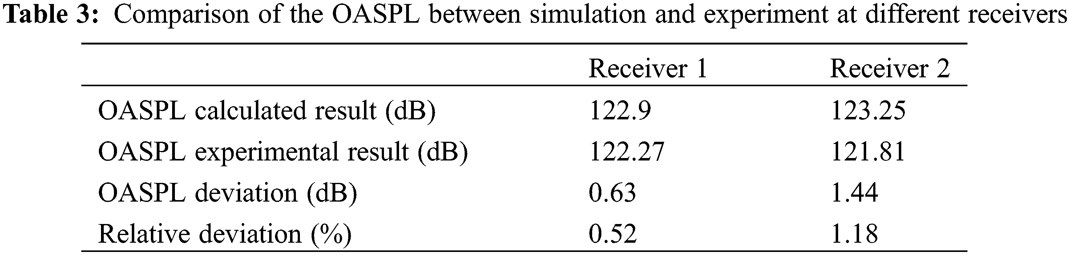
The numerical simulation method in this paper is used to calculate the verification model and obtain calculated results. Figs. 4a and 4b are the frequency spectrum of the sound pressure level of calculated results and experimental results at receiver 1 and receiver 2, respectively. It can be seen from Fig. 4 that the sound pressure level spectrum trends of calculated results and experimental results are substantially the same. The overall sound pressure level comparison between the experimental results and the calculated results is shown in Table 3. The relative deviation is 0.52% and 1.18% at receiver 1 and receiver 2, respectively, and the average relative deviation is 0.85%, indicating that the numerical simulation method is feasible and accurate.

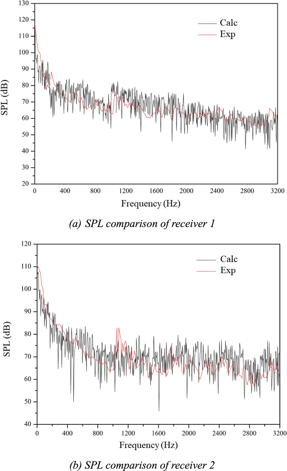
Figure 4: Comparison of calculated results and experimental results

3  Results and Discussion

In this section, the distribution of pressure, velocity and sound source intensity in the flow channel is investigated first, and then the modal analysis of the flow channel is carried out. Besides, the characteristics of excitation force and structure-borne noise are considered. Finally, the influence of flow velocity on flow-induced noise and structure-borne noise are researched comparatively.

3.1 Flow Field Analysis

To explore structure-borne noise, an analysis of the flow field inside the flow channel is first presented. Distribution of pressure and velocity at v = 3 m/s are shown in Figs. 5 and 6, respectively. Fig. 5 portrays that the pressure is the highest at the inlet section and the lowest at the outlet section, and the pressure changes drastically at the variable cross-section area. A low-pressure area is located in the corner of the variable cross-section and near the wall, which indicating that there is vortex generation. Fig. 6 indicates that flow velocity increases drastically at the variable cross-section area, from 3 to 12 m/s.

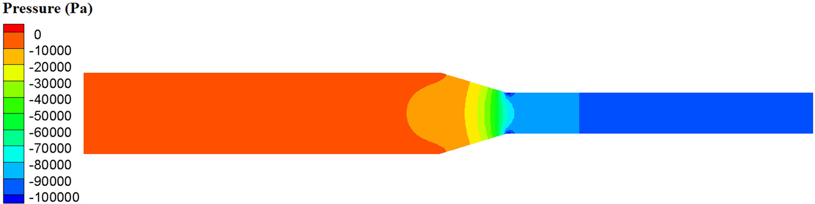
Figure 5: Pressure distribution of flow channel at v = 3 m/s

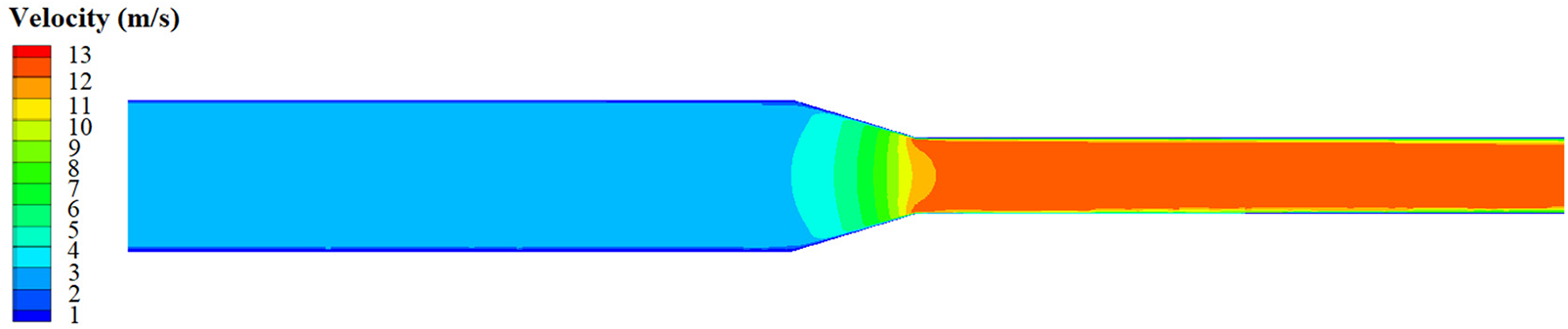
Figure 6: Velocity distribution of flow channel at v = 3 m/s

Acoustic source intensity distribution is shown in Fig. 7. It can be seen from the figure that the main sound source area overlaps with the low-pressure area. When the fluid flows through the variable cross-section, vortices are generated at the corner of the variable cross-section. According to the theory of vortex sound [30,31], the stretching, deformation, dissipation, and collapse of the vortex in the flow field all produce sound. The acoustic source intensity at the vortices and nearby the vortices areas is significantly greater than that in other areas. Thus, the pressure pulsation and vortices at the corner of variable cross-section is the main sound source of flow-induced noise.

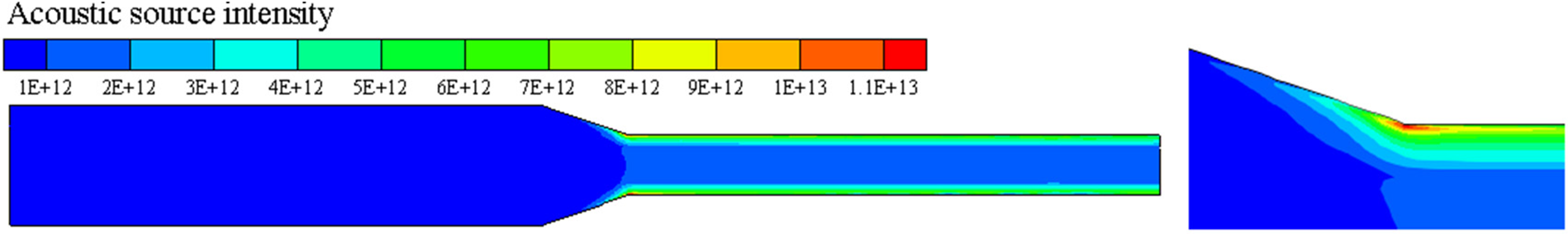
Figure 7: Acoustic source intensity distribution of flow channel

3.2 Mode Shape Analysis

In this paper, the flow channel with variable cross-section is rigidly connected as a whole. The modal information and structure-borne noise is extracted using ANSYS Mechanical. Constraint conditions of flow channel adopt free edge constraints at both ends to restrict the three constraint directions X, Y, and Z, as shown in Fig. 8.

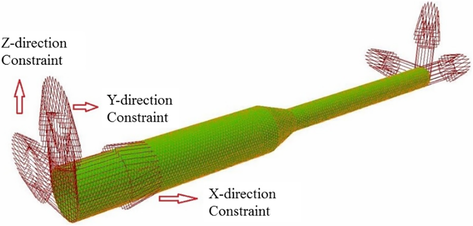
Figure 8: Constraint of the flow channel with variable cross-section

As the result of the modal analysis, typical mode shapes are obtained, as shown in Fig. 9. The red area is the maximum displacement. The first frequency is 859.21 Hz, and the maximum displacement is located in the variable cross-section area. This area is also the main sound source area and where the excitation force is concentrated. The second frequency is 2377.06 Hz, and the main displacement is located in the middle of the outlet flow channel. Since the noise frequency in this study is from 0 to 3000 Hz, the research is focused on the first and second mode.

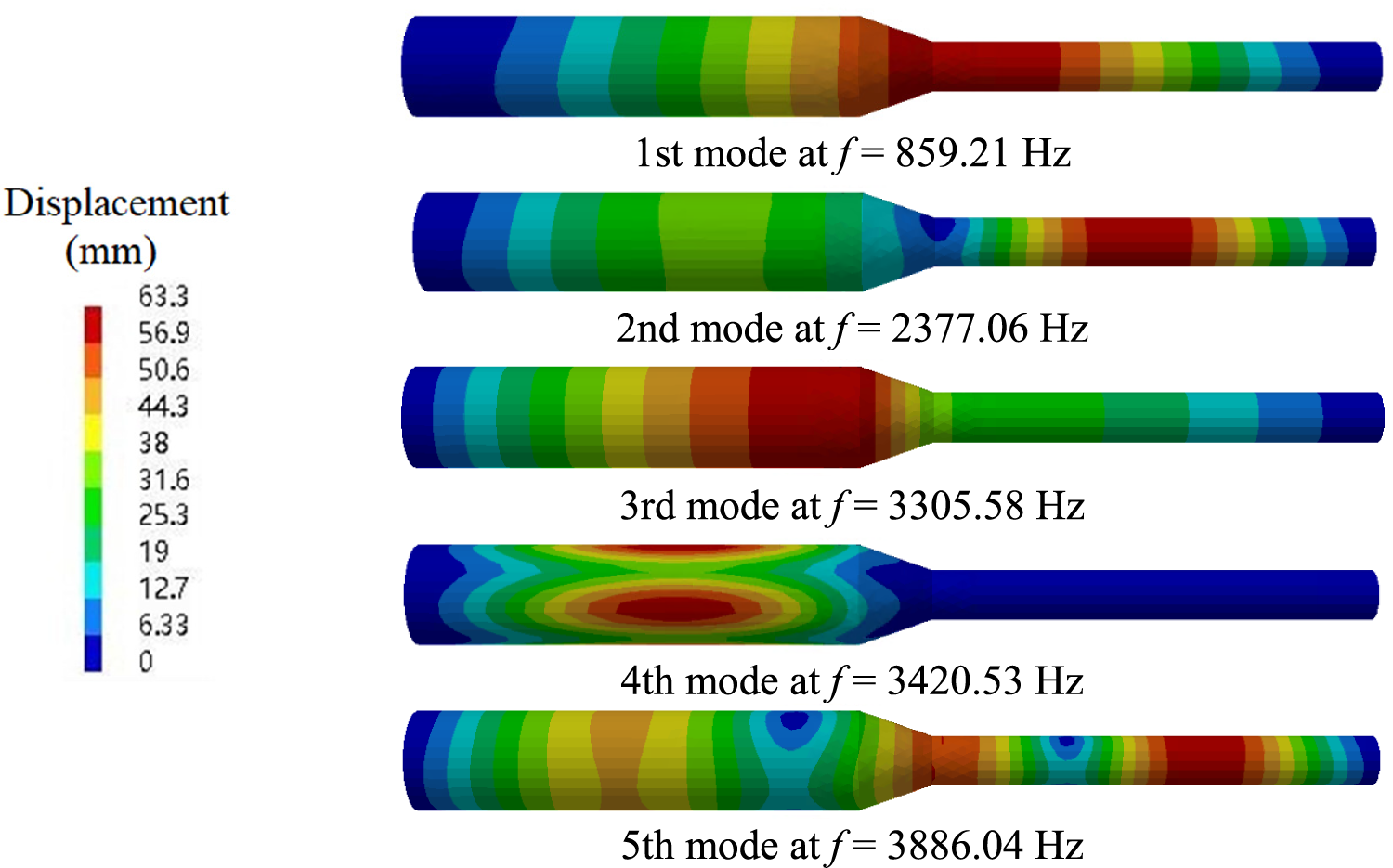
Figure 9: Typical mode shapes of modal analysis

3.3 Analysis of Excitation Force on the Flow Channel Wall

The exciting force is the force that makes the vibrating body vibrate. As a result, the exciting force acting on the flow channel wall mainly comes from the pressure pulsation generated by the unsteady flow of the fluid in the flow channel. Thus, in the transient flow field calculation, it is necessary to monitor the pressure pulsations and the excitation force on the wall.

Figs. 10a–10f are the average excitation force curves of flow channel wall in time domain and frequency domain at v = 1 m/s, v = 2 m/s, and v = 3 m/s, respectively. The average excitation force at different velocities presents a cyclical trend in time domain. The pulsation range of the average excitation force gradually expands with the increase of the flow velocity. When the flow velocity increases from 1 to 3 m/s, the pulsation range is expanded from 0.6–1.1 N to 7–15 N. In the frequency domain, the excitation force response characteristics are the same at different flow velocities, and the fluctuations decrease with the increase of frequency. The maximum excitation force is in the range of 0 to 20 Hz. When the frequency is higher than 1000 Hz, the excitation force is almost 0. The maximum excitation force and the amplification of the maximum excitation force increase as the flow velocity increases.

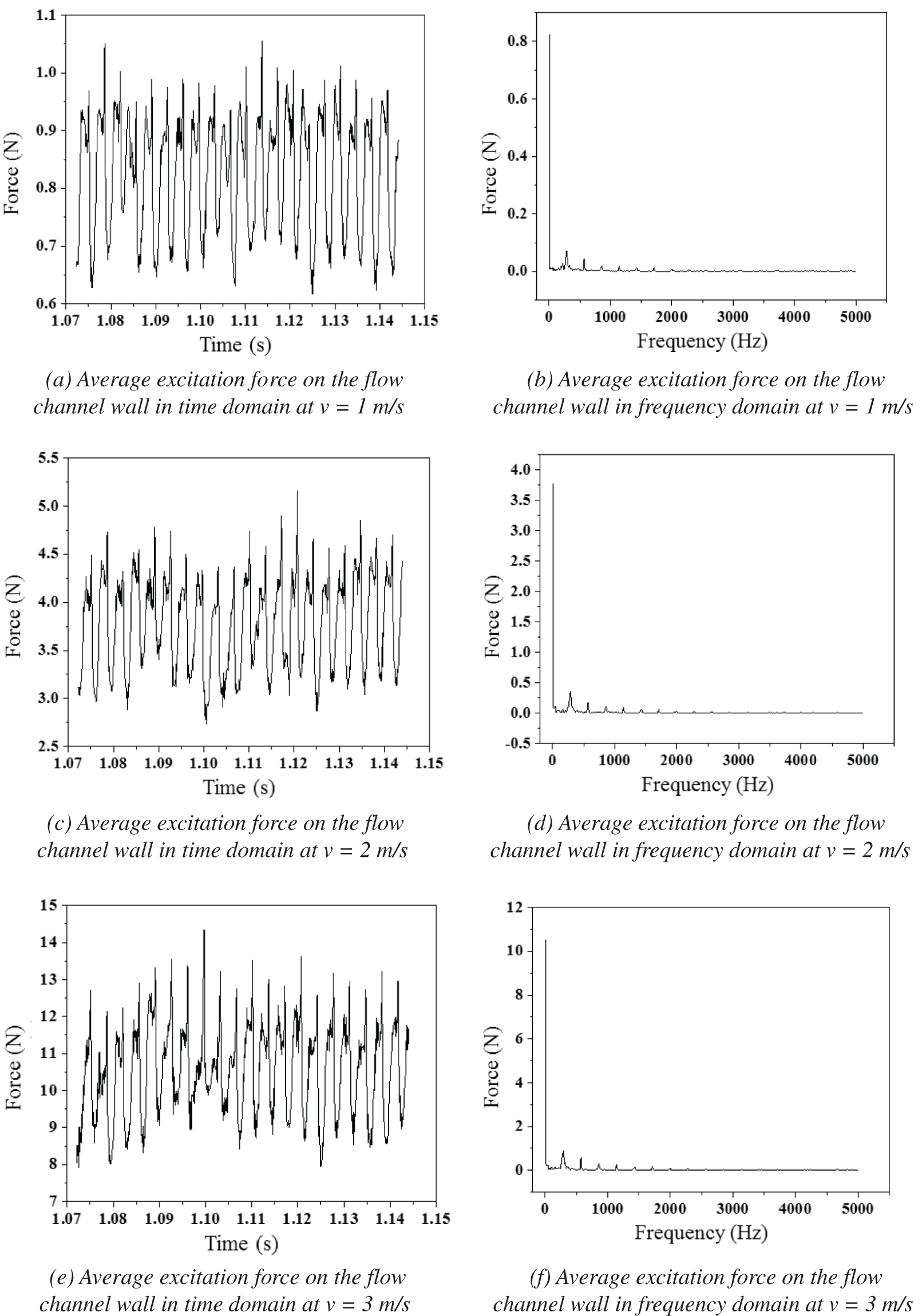
Figure 10: Excitation force on flow channel wall in time domain and frequency domain

3.4 Analysis of Structure-Borne Noise

Excitation force is applied to the inner wall of the flow channel, and the vibration response is calculated based on the modal analysis theory. Fig. 11 describes the equivalent stress on the flow channel at the first and second frequency, respectively. It can be seen in Fig. 11 that the maximum equivalent stress at the first frequency is 326 Pa, and the maximum equivalent stress appears in the variable cross-section area and the first half of the outlet flow channel section. At the second frequency, the maximum equivalent stress reduces to 13.5 Pa. Compared with the equivalent stress at the first frequency, the equivalent stress at the second frequency contributes very little to the total equivalent stress. Therefore, the first frequency is the main frequency of vibration and structure-borne noise.

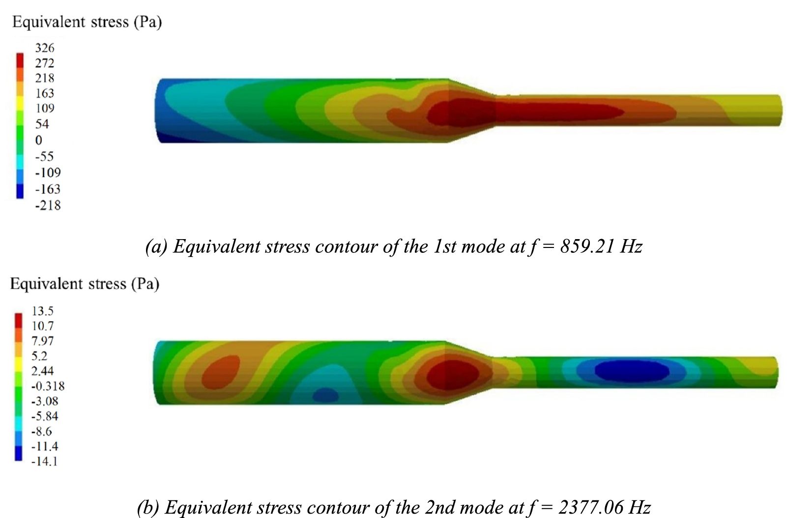
Figure 11: Equivalent stress on the flow channel at v = 3 m/s

In order to deeply study the variation of the maximum equivalent stress with the flow velocity at the first and second frequencies, the maximum equivalent stress corresponding to each flow velocity is calculated, as shown in Table 4.

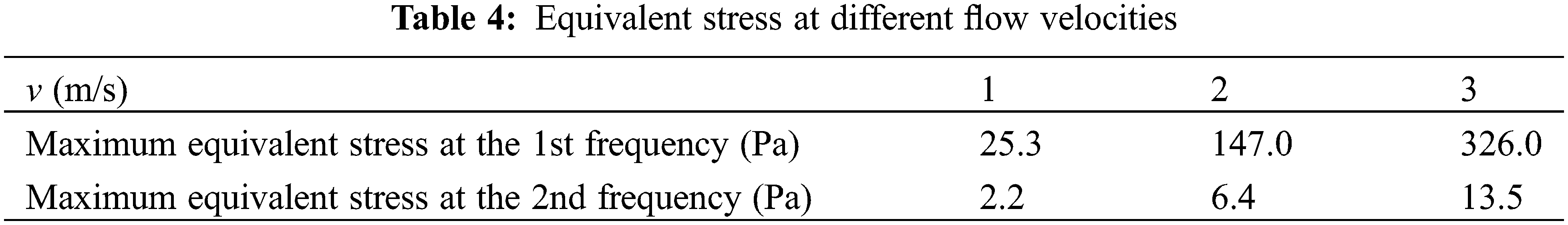
Table 4 indicates that the maximum equivalent stress at both the first and second frequencies increases with the increase of the flow velocity. It is consistent with the previous analysis of excitation force and mode shapes. When the flow velocity increases, the increase in excitation force is the cause of the increase in equivalent stress. The displacement of the first mode is greater than the displacement of the second mode, which can explain that the equivalent stress at the first frequency is greater than the equivalent stress at the second frequency.

Fig. 12 reports the SPL of structure-borne noise at different velocities based on modal calculation. Fig. 12 illustrates that the trend of spectrum with two obvious peaks at different flow velocities is the basic similar, corresponding to the first frequency of 859.21 Hz and the second frequency of 2377.06 Hz.

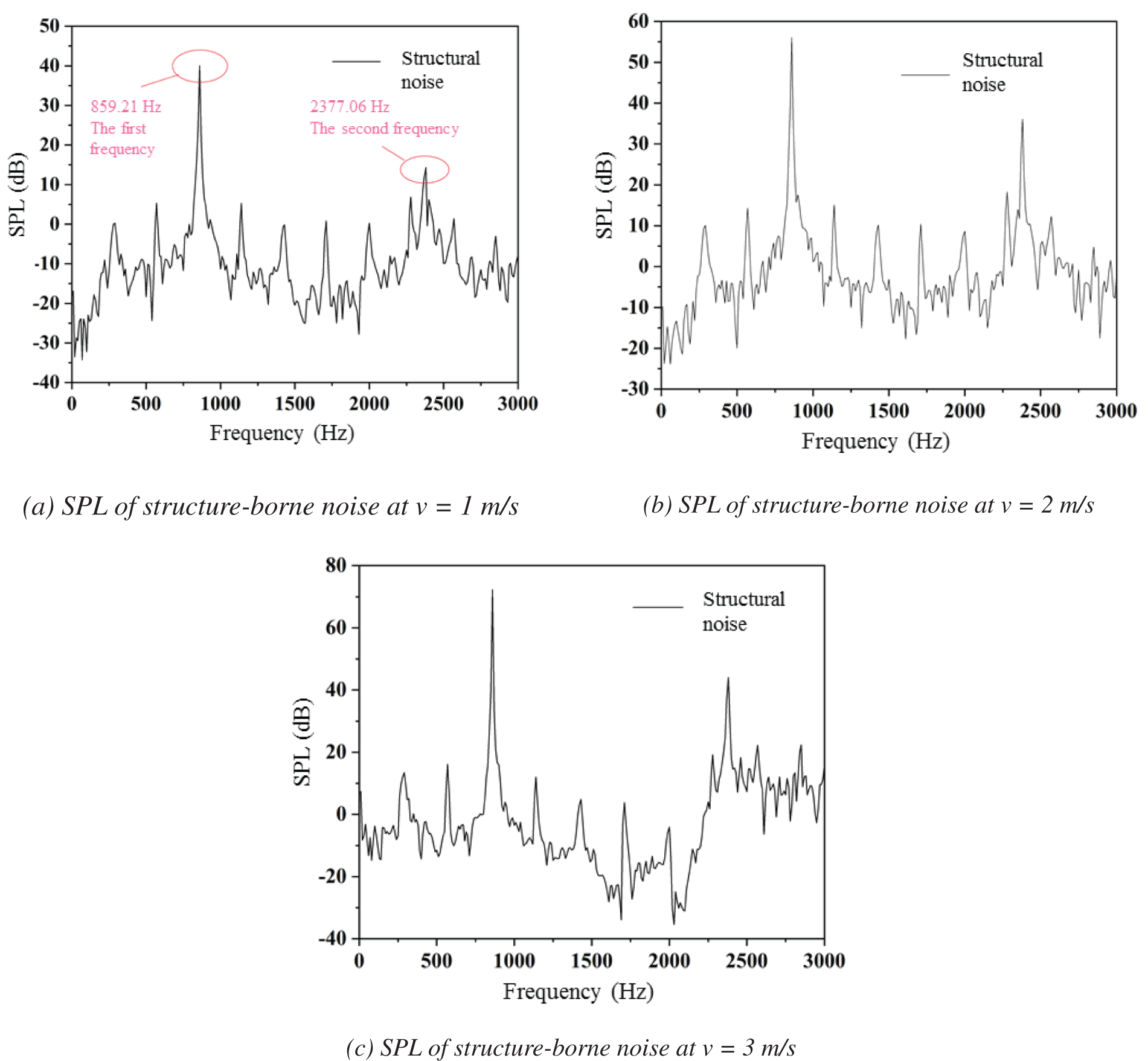
Figure 12: SPL of structure-borne noise at different velocities

3.5 Influence of Flow Velocity on Flow-Induced Noise and Structure-Borne Noise

In order to research the influence of flow velocity on structure-borne noise and flow-induced noise, the SPL of structure-borne noise and flow-induced noise at different velocities are researched comparatively, as shown in Table 5.

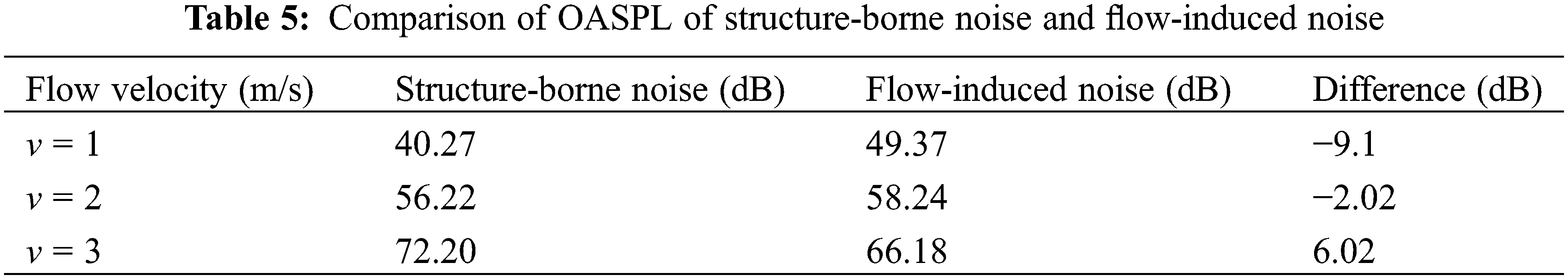
Table 5 illustrates that as the flow velocity rises from 1 to 3 m/s, the OASPL of flow-induced noise rises from 49.37 to 66.37 dB, and the OASPL of structure-borne noise rises from 40.27 to 72.20 dB. Both structure-borne noise and flow-induced noise increase with the increase of flow velocity, and the increment of structure-borne noise is greater than that of flow-induced noise.

4  Conclusions

This paper firstly established the numerical calculation model of fluid-structure interaction noise. Then, based on the finite element method and modal analysis theory, the generation of flow-induced noise, mode shapes and structure-borne noise of the variable-section flow channel at different flow rates were investigated. The main conclusions are as follows:

(1) The first to fifth mode shapes of the flow channel are obtained, and the frequencies are 859.21, 2377.06, 3305.58, 3420.53, 3886.04 Hz, respectively. The maximum displacement and equivalent stress are located in the variable cross-section area.

(2) The spectral trends of structure noise under different flow rates are basically similar, and there are two obvious peaks, corresponding to the first frequency of 859.21 Hz and the second frequency of 2377.06 Hz, respectively. The average excitation force showed a periodic trend, and the pulsation range gradually increased with the increase of the flow velocity. The pulsation range expanded from 0.6–1.1 N to 7–15 N when the flow rate was increased from 1 to 3 m/s.

(3) The main sound source area of the flow-induced noise overlaps with the low-pressure area, and is located on the wall at the corner of the variable cross-section. The main sound source of structure-borne noise is located in the variable cross-section, which is the area with the maximum modal displacement and equivalent stress.

(4) As the flow velocity rises from 1 to 3 m/s, the OASPL of flow-induced noise rises from 49.37 to 66.37 dB, and the OASPL of structure-borne noise rises from 40.27 to 72.20 dB. Both structure-borne noise and flow-induced noise increase with the increase of flow velocity, and the increment of structure-noise is greater than that of flow-induced noise.

Funding Statement: This work is supported by the Key Research and Development Project of Shandong Province [2019GSF109084], the National Natural Science Foundation of China [51776111] and Young Scholars Program of Shandong University [2018WLJH73].

Conflicts of Interest: The authors declare that they have no conflicts of interest to report regarding the present study.

References

1. Rao, A. R., Padmavathi, K. (1993). Pulsatile flow of a viscous fluid in elliptical pipe of variable cross-section. International Journal of Non-Linear Mechanics, 28(4), 455–466. [Google Scholar]

2. Andrea, L. S., Martin, K., Matteo, G., Wolfgang, A. W., Antonio, H. (2020). A weakly compressible hybridizable discontinuous Galerkin formulation for fluid-structure interaction problems. Computer Methods in Applied Mechanics and Engineering, 372(17), 113392. [Google Scholar]

3. Li, Z., Cao, W., Le, T. D. (2019). On the coupling of a direct-forcing immersed boundary method and the regularized lattice Boltzmann method for fluid-structure interaction. Computers & Fluids, 190(4), 470–484. [Google Scholar]

4. Wang, L., Tian, F. B., Lai, J. C. (2020). An immersed boundary method for fluid-structure-acoustics interactions involving large deformations and complex geometries. Journal of Fluids and Structures, 95(6), 102993. [Google Scholar]

5. Yu, W., Zeng, H., Li, M., Wang, Z. (2008). The characteristics and measurement of noise from pipeline of pipe gallery oxygen areas in large iron and steel plants. Environmental Engineering, 26, 68–70. [Google Scholar]

6. Coombs, J. L., Schembri, T. J., Zander, A. C. (2020). Pipeline blowdown noise levels and noise modelling. Applied Acoustics, 168(1), 107405. [Google Scholar]

7. Guo, C., Gao, M. (2020). Investigation on the flow-induced noise propagation mechanism of centrifugal pump based on flow and sound fields synergy concept. Physics of Fluids, 32(3), 035115. [Google Scholar]

8. Liang, X. (2010). Study on the technique for measuring noise in pipelines. Noise Vibrationss Control, 30, 123–124+128. [Google Scholar]

9. Aladwani, A., Almandeel, A., Nouh, M. (2019). Fluid-structural coupling in metamaterial plates for vibration and noise mitigation in acoustic cavities. International Journal of Mechanical Sciences, 152(5), 151–166. [Google Scholar]

10. Xu, Z., He, W., Xin, F., Lu, T. (2020). Sound propagation in porous materials containing rough tubes. Physics of Fluids, 32(9), 093604. [Google Scholar]

11. Kojima, T., Inaba, K. (2020). Numerical analysis of wave propagation across Solid-Fluid interface with Fluid-Structure interaction in circular tube. International Journal of Pressure Vessels and Piping, 183, 104099. [Google Scholar]

12. Cheng, Y., Oertel, H., Schenkel, T. (2005). Fluid-structure coupled CFD simulation of the left ventricular flow during filling phase. Annals of Biomedical Engineering, 33(5), 567–576 [Google Scholar] [PubMed]

13. Kim, H., Lee, S., Son, E., Lee, S., Lee, S. (2012). Aerodynamic noise analysis of large horizontal axis wind turbines considering fluid-structure interaction. Renewable Energy, 42, 46–53. [Google Scholar]

14. Liu, G., Li, Y. (2011). Vibration analysis of liquid-filled pipelines with elastic constraints. Journal of Sound and Vibration, 330(13), 3166–3181. [Google Scholar]

15. Li, W., Wang, W., Yan, Y., Yu, Z. (2020). A strong-coupled method combined finite element method and lattice Boltzmann method via an implicit immersed boundary scheme for fluid structure interaction. Ocean Engineering, 214(6), 107779. [Google Scholar]

16. Han, N., Mai, Z. (2006). Estimation of breakout sound power level due to turbulence caused by an in-duct element. Technical Acoustics, 25(6), 653–657. [Google Scholar]

17. Liu, E., Yan, S., Wang, D., Huang, L. (2015). Large eddy simulation and FW-H acoustic analogy of flow-induced noise in elbow pipe. Journal of Computational and Theoretical Nanoscience, 12(9), 2866–2873. [Google Scholar]

18. Han, T., Wang, L., Cen, K., Song, B., Shen, R. et al. (2020). Flow-induced noise analysis for natural gas manifolds using LES and FW-H hybrid method. Applied Acoustics, 159(10), 107101. [Google Scholar]

19. Hambric, S. A., Boger, D. A., Fahnline, J. B., Campbell, R. L. (2010). Structure and fluid-borne acoustic power sources induced by turbulent flow in 90 degrees piping elbows. Journal of Fluids and Structures, 26(1), 121–147. [Google Scholar]

20. Mori, M., Masumoto, T., Ishihara, K. (2017). Study on acoustic, vibration and flow induced noise characteristics of T-shaped pipe with a square cross-section. Applied Acoustics, 120(5), 137–147. [Google Scholar]

21. Zhao, W., Peng, X., Chen, M., Li, Q. (2016). Numerical simulation of flow-induced noise in the pipelines with variable cross-sections. Noise Vibration Control, 36, 48–51+150. [Google Scholar]

22. Williams, J. F., Hawkings, D. (1969). Theory relating to the noise of rotating machinery. Journal of Sound and Vibration, 10(1), 10–21. [Google Scholar]

23. Guo, H., Guo, C., Hu, J., Lin, J., Zhong, X. (2021). Influence of jet flow on the hydrodynamic and noise performance of propeller. Physics of Fluids, 33(6), 065123. [Google Scholar]

24. Sun, L., An, C., Wang, N., Zhe, C., Wang, L. et al. (2021). Effect of the rotor blade installation angle on the structure-borne noise generated by adjustable-blade axial-flow fans. Physics of Fluids, 33(9), 095107. [Google Scholar]

25. Itoh, Y., Tamura, T. (2008). Large eddy simulation of turbulent flows around bluff bodies in overlaid grid systems. Journal of Wind Engineering and Industrial Aerodynamics, 96(10–11), 1938–1946. [Google Scholar]

26. Li, C., Yan, S., Wen, D., Huang, Q., Lin, Y. (2018). CFD analysis of flow noise at tees at natural gas station. Noise Control Engineering Journal, 66(1), 1–10. [Google Scholar]

27. Queguineur, M., Bridel-Bertomeu, T., Gicquel, L. Y., Staffelbach, G. (2019). Large eddy simulations and global stability analyses of an annular and cylindrical rotor/stator cavity limit cycles. Physics of Fluids, 31(10), 104109. [Google Scholar]

28. Es-Sahli, O., Sescu, A., Afsar, M. Z., Buxton, O. R. (2020). Investigation of wakes generated by fractal plates in the compressible flow regime using large-eddy simulations. Physics of Fluids, 32(10), 105106. [Google Scholar]

29. Lv, J., Ji, Z. (2011). Study on prediction and experimental measurment of flow noise in pipes with variable cross-section area. Noise Vibration Control, 31, 166–169. [Google Scholar]

30. Powell, A. (1964). Theory of vortex sound. The Journal of the Acoustical Society of America, 36(1), 177–195. [Google Scholar]

31. Guo, C., Gao, M., Wang, J., Shi, Y., He, S. (2019). The effect of blade outlet angle on the acoustic field distribution characteristics of a centrifugal pump based on Powell vortex sound theory. Applied Acoustics, 155, 297–308. [Google Scholar]