Computational-Analysis of the Non-Isothermal Dynamics of the Gravity-Driven Flow of Viscoelastic-Fluid-Based Nanofluids Down an Inclined Plane

Nomenclature

1  Introduction

Dispersion of thermally conductive, tiny metallic particles within a fluid (such as water, oil, etc.) is the most obvious and effective method of improving/enhancing the heat-transfer-rate (HTR) characteristics and thermal-conductivity properties of the fluid. The size and texture of the metallic particles are clearly fundamental; large particles can lead to sedimentation, clogging, etc., while coarse-grained particles can cause abrasion, etc. For these reasons, nanometer-size particles (nanoparticles) are used [1–24].

As in the cited references, the term nanofluid is herein used to describe the suspension of solid nanoparticles in a base fluid. A variety of industrial applications (say heating and cooling) and medical applications (chemotherapy, etc.) of nanofluids are well documented in the literature and summarized by the cited references. Noting the fundamental importance of the rheology of the base fluid to the modern applications of nanofluids, the studies, say in [1–3] focus attention on non-Newtonian (specifically polymeric) base-fluids under various flow conditions. The widespread importance of non-Newtonian fluids, both the Generalized Newtonian Fluids (GNF) as well as the polymeric (viscoelastic) fluids, in contemporary application is quite straightforward for example [1–3,6,8,25–34].

The current study builds on the investigations in [1–3] and extends these investigations to free-surface, gravity-driven, thin-film flows with convective heat exchange at the free-surface. Additionally and alternatively, the current work extends the combined (particle-free) fluid-dynamics studies in [25] and [29] to the inclusion of solid nanoparticles and hence raising the cited works to nanofluid-dynamics.

The current work employs solution methodologies based on semi-implicit numerical-schemes derived from the finite difference methods (FDM). The computational solution algorithms are implemented in the MATLAB software. It is noted that other alternative numerical methodologies have been utilized for the computational solution processes of similar nanofluid flow problems. Such alternative numerical methodologies have been applied for hybrid nanofluid flow [35,36], for fractional viscoelastic fluid [37,38], and for fractional viscoelastic hybrid nanofluid [39]. For example, the work in [40] investigates a Generalized Newtonian fluid (the Casson fluid) based nanofluid subjected to thermal radiation, Joule heating, and magnetic effects flowing over an inclined porous stretching sheet. Similar work in [41] investigates thermal and velocity slip effects on Casson nanofluid flow over an inclined permeable stretching cylinder via collocation methods. The work in [42] gives an extensive review of strategies based, among others, on nanofluids for solving “internal heat generation problem” for the optimization of heat transfer in electronic devices. The work in [43] explores the significant potential of nanofluids, and specifically the influence of nano-particle size and distribution, in solar energy harvesting. The importance of viscoelastic fluid in heat generation/absorption is also explored in [44] using Maxwell fluids.

The following sequence is adopted in the paper. Section 2 outlines the description of the physical and mathematical models. The development and implementation of the numerical and computational algorithms as well as the real efficacy, accuracy, and convergence of the computational methodologies are given in Section 3. The main results are presented graphically and discussed qualitatively in Section 4. Concluding remarks follow in Section 5.

2  Problem Formulation

A schematic of the model problem is sketched in Fig. 1. A thin film of nanofluid (VFBN) of height h∗ (where the height is in the direction normal to the inclined wall) flows down an inclined plane. The inclined wall/plane makes an angle θ with the horizontal.

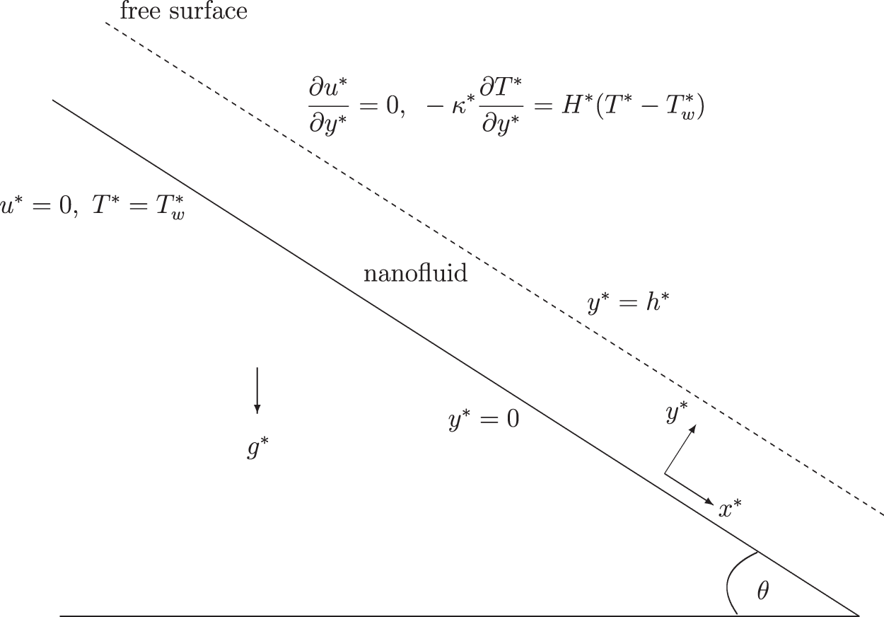
Figure 1: Schematic of the model problem

The x∗ -axis is taken parallel to the inclined wall and the y∗ -axis is taken perpendicular to this incline. The superscript ( ∗ ) denotes dimensional variables. The variables and parameters are otherwise similar to those described in [1–3].

The solid boundary (the inclined wall) is kept at a constant temperature Tw∗ and convective cooling is assumed at the free-surface, governed by Newton’s law of cooling.

The motion of the fluid is exclusively gravity-driven and hence the pressure gradient in the x∗ -direction stays zero. Alternatively the pressure in the x∗ -direction stays constant. Naturally, the pressure in the y∗ -direction is non-constant increasing from atmospheric pressure at the free surface to the maximum fluid pressure at the bottom, i.e., at the inclined wall.

No-slip velocity boundary conditions are assumed along the rigid inclined wall. The velocity boundary conditions at the free-surface naturally also arise from the zero-shear-rate requirements.

Following the notations of [1–3,29], the governing PDEs (in dimensional form) for the VFBN are,

∇∗⋅u∗=0, (1)

ρnf∗Du∗Dt∗=−∇∗p∗+∇∗⋅(σ∗)+ρnf∗g∗F, (2)

(ρcp)nf∗DT∗Dt∗=−∇∗⋅ϕq∗+QD∗+r∗. (3)

Here F=(sin⁡θ,−cos⁡θ) denotes the body force due to gravity and g∗ is the acceleration due to gravity. The heat-source terms, denoted by r∗ , will subsequently be neglected in this study as their effects have been comprehensively investigated in previous studies, as in [1].

Dimensionless parameters

The equations are studied in non-dimensional form via the following dimensionless-parameters; Deborah-number (De), Reynolds-number (Re), Prandtl-number (Pr), Brinkman-number (Br), Peclet-number (Pe = Re ⋅ Pr), activation-energy parameter ( α ), Grashof-number (Gr), Biot-number (Bi), and ( β ) which represents the proportion of the polymer-viscosity compared to the fluid’s total-viscosity. These are defined as follows:

β=ηp∞∗η∞∗,De=λ∞∗U∞∗h∗,Re=ρf∗h∗U∞∗η∞∗,Pr=η∞cpf∗∗κf∗,Br=U∞∗2η∞∗κf∗αTW∗,Renf=ρnfρfRe,Penf=(ρcp)nf(ρcp)fPe,α=R∗TW∗E∗,Gr=g∗h∗U∞∗,Bi=H∗h∗k0∗. (4)

The subscript ( nf ) depicts nanofluid and the appropriate (nanofluid) quantity is obtained linearly from contributions of the base-fluid volume-fractions ( f ) and the nanoparticles ( s ) volume-fractions,

ρnf=φρs+(1−φ)ρf,(cpρ)nf=φ(cpρ)s+(1−φ)(cp,ρ)f,

where, φ is the volume fraction function. The resultant dimensionless governing equations are,

∇⋅u=0, (5)

RenfDuDt=−Renf∇p+∇⋅(σ)+RenfGrF, (6)

PenfDTDt=−∇⋅(κnf∇T)+BrQD, (7)

τ+ετ2+λ¯(T)De[ τ∇ − τDDt(ln(αT+1)) ]=ηp(T)(1−φ)5/2S.(8)

The expression for the appropriate mechanical dissipation term is,

QD=γτ:S+(1−γ)ηs(T)(1−φ)5S:S. (9)

As given in [1], the expressions for viscosities, relaxation-times, and thermal-conductivities, under non-isothermal conditions are,

ηs(T)=(1−β)e(−αT),(ηs)nf=ηs(T)(1−φ)5/2, (10)

ηp(T)=βe(−αT),(ηp)nf=ηp(T)(1−φ)5/2, (11)

η=ηp(T)+ηs(T),ηnf=η(1−φ)5/2, (12)

λ¯(T)=1αT+1e(−αT), (13)

κnf=κs−(ℵ−1)φ(κf−κs)+(1−ℵ)κfκs+φ(κf−κs)+(1−ℵ)κf(1+αA2T). (14)

2.1 Boundary and Initial Conditions

The start-up conditions (at time t = 0) and the wall-conditions (at the inclined wall, y = 0, and at the free-surface, y = 1) are,

T(0,y)=0,u(0,y)=0,τ(0,y)=0,0≤y≤1, (15)

u(t,0)=0,T(t,0)=0,∂∂yu(t,1)=1,∂∂yT(t,1)=−BiT(t,1),t≥0. (16)

Due to the hyperbolic nature of the equations for the polymeric stresses, the relevant boundary-conditions for these equations are reconstructed from the main flow [1–3,29].

3  Numerical Solution

The numerical-scheme adopted for the velocity component is derived from a semi-implicit FDM approach,

Renfu(n+1)−u(n)Δt=(ηs)nf(n)∂2∂y2u(n+ξ)+∂∂yτ12(n)+∂∂yu(n)∂∂y(ηs)nf(n)+RenfGrsin⁡θ, (17)

where

u(n+ξ)=(1−ξ)u(n)+ξu(n+1).

The velocity therefore updates at the new time-level, u(n+1) , via the recursive algorithm,

−r1uj−1(n+1)+(Renf+2r1)uj(n+1)−r1uj+1(n+1)=Renfuj(n)+(1−ξ)Δt(ηs)nf(n)∂2∂y2u(n)+Δt((1−β)∂∂y(ηs)nf(n)∂∂yu(n)+∂∂yτ12(n)+ΔtRenfGrsin⁡θ), (18)

where

r1=ξ(ηs)nf(n)ΔtΔy2.

This represents a (diagonally-dominant) tri-diagonal linear algebraic system of equations. The discretized temperature equation is obtained similarly,

Penf∂T∂t=κnf(n)∂2∂y2T(n+ξ)+∂∂yT(n)∂∂yκnf(n)+BrQD(n). (19)

The temperature therefore updates at the new time-level, T(n+1) , via the recursive algorithm,

−r2Tj−1(n+1)+(Penf+2r2)Tj(n+1)−r2Tj+1(n+1)=PenfTj(n)+(1−ξ)Δtκnf∂2∂y2T(n)+Δt∂∂yT(n)∂∂yκnf(n)+2(1−γ)ΔtBr(ηs)nf(n)(∂∂yu(n))2+2ΔtBrγτ12(n)∂∂yu(n), (20)

where

r2=ξκnf(n)ΔtΔy2.

The semi-implicit numerical scheme for the polymeric-stress, τ is,

τ(n+ξ)+ε(τ2)(n)+λ¯(n)Deτ(n+1)−τ(n)Δt=explicitterms.

The solutions for the tensor components, τ11(n+1) , τ12(n+1) , and τ22(n+1) therefore follow directly from algebraic manipulation,

(Deλ¯(n)+ξΔt)τ(n+1)=explicit‐terms. (21)

The explicit-terms for τ11 , τ12 and τ22 are respectively,

[λ¯(n)De−(1−ξ)Δt]τ11(n)+Δtλ¯(n)De[τ12(n)∂∂yu(n)+τ11(n)∂∂ylog⁡(1+αT(n))]−εΔt(τ112+τ122), (22)

[λ¯(n)De−(1−ξ)Δt]τ12(n)+Δtλ¯(n)De[τ22(n)∂∂yu(n)+τ12(n)∂∂ylog⁡(1+αT(n))]+Δt(ηp)nf∂∂yu(n)−εΔt(τ11τ12+τ12τ22), (23)

[λ¯(n)De−(1−ξ)Δt]τ22(n)+Δtλ¯(n)Deτ22(n)∂∂ylog⁡(1+αT(n))−εΔt(τ122+τ222). (24)

4  Results

Graphical results are presented for the VFBN temperature field (T), velocity field (u), and polymeric-stress components ( τ11,τ12andτ22 ), using the below list of default values,

α=0.01,Br=1,Prnf=1,Renf=1,Bi=1,Gr=1,De=2,β=0.2,γ=0.5,Δy=0.01,Δt=0.1,θ=45,t=50,ζ=1,φ=0.04,A2=0.2,ε=1,ℵ=3. (25)

4.1 Time Devolvement of Steady Solutions

The time development of flow variables from the initial states until steady solutions are reached, as is illustrated in Figs. 2 and 3. It can be noted that all solutions stably and ultimately settle to consistent steady states.

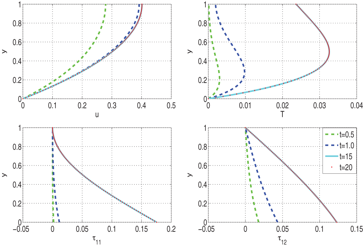
Figure 2: Time-development of profiles to steady-state with Δt=0.05

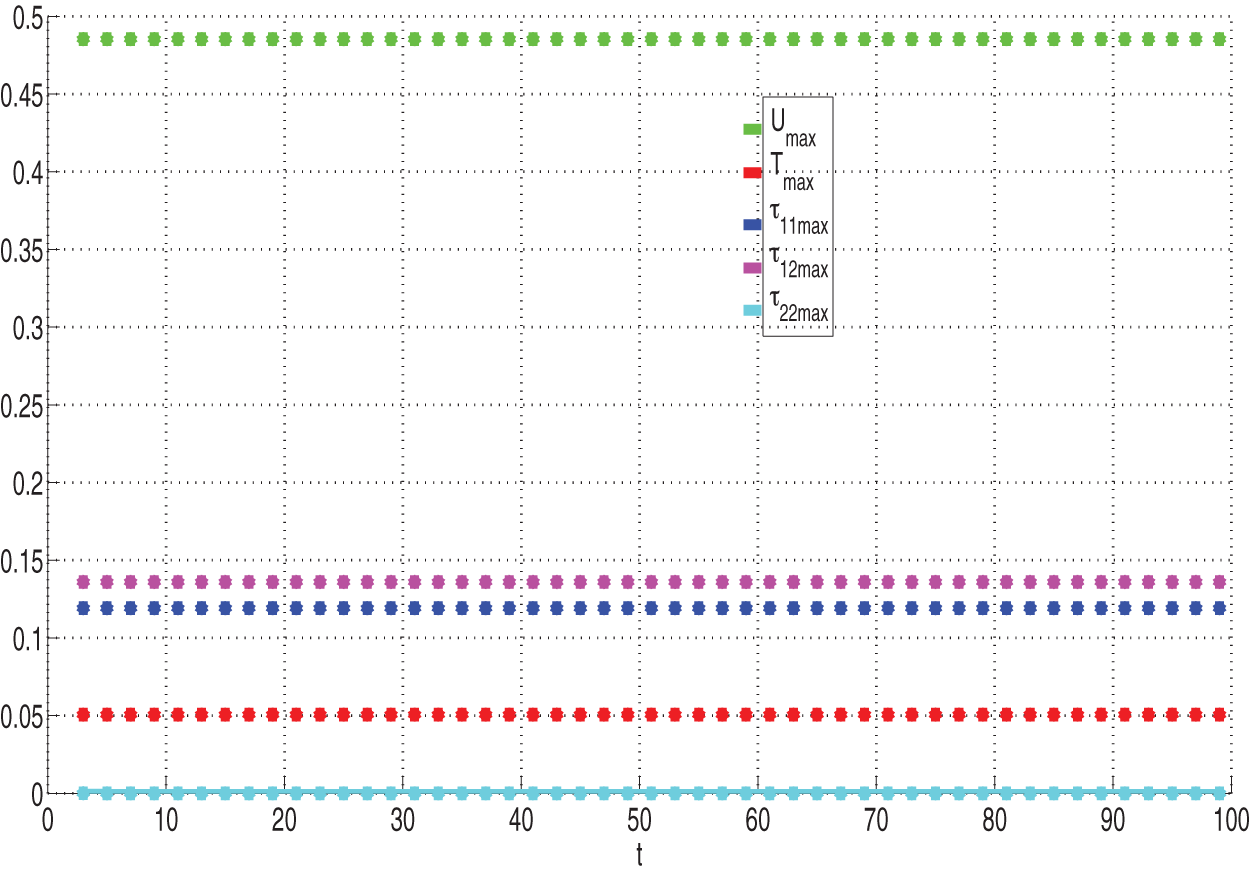
Figure 3: Time development of maximum flow quantities to steady-state

4.2 Time-Step and Mesh Size Convergence

Figs. 4–7 illustrate that the computational and numerical algorithms are independent of both time-step size and mesh size as required. The computational and numerical scheme specifically, and efficiently, reproduce the required steady-solutions for a wide range of expected time-step sizes and mesh sizes.

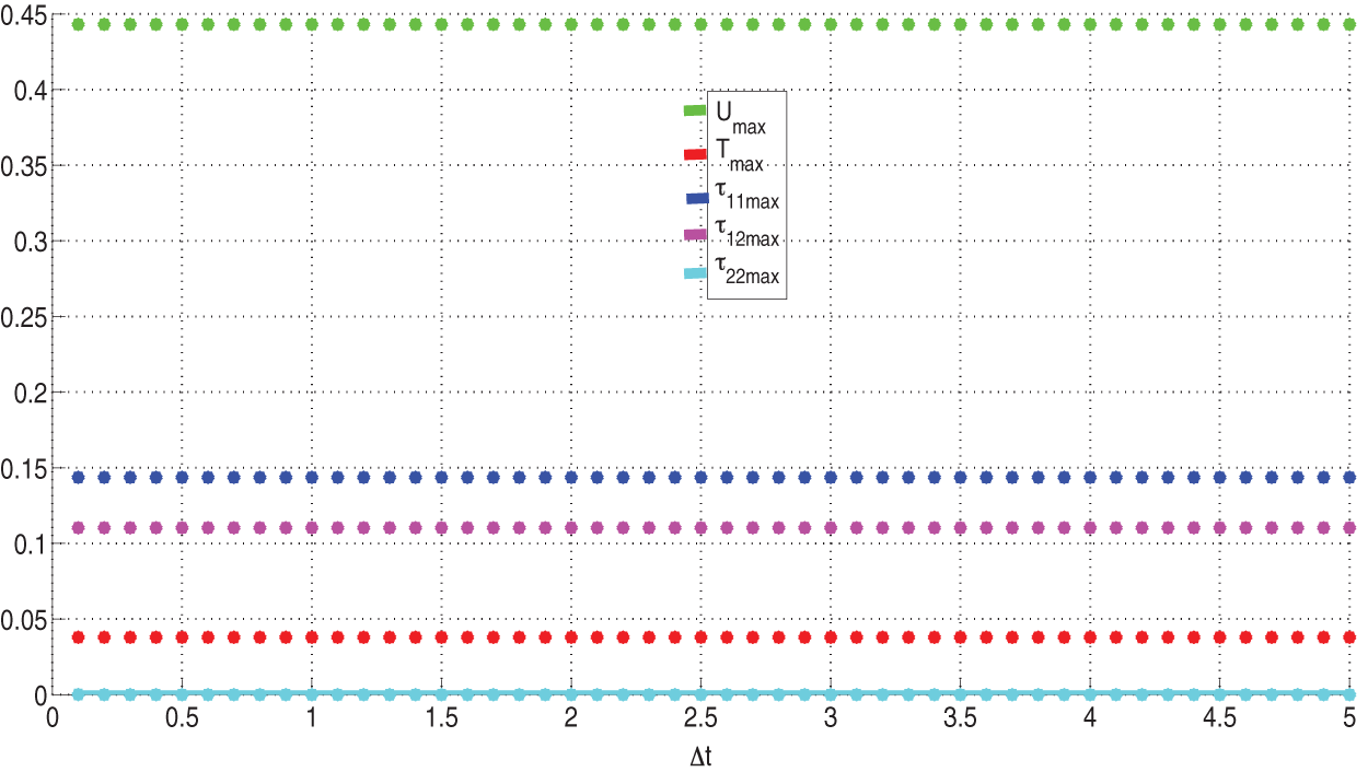
Figure 4: Time-step independence of maximum solutions

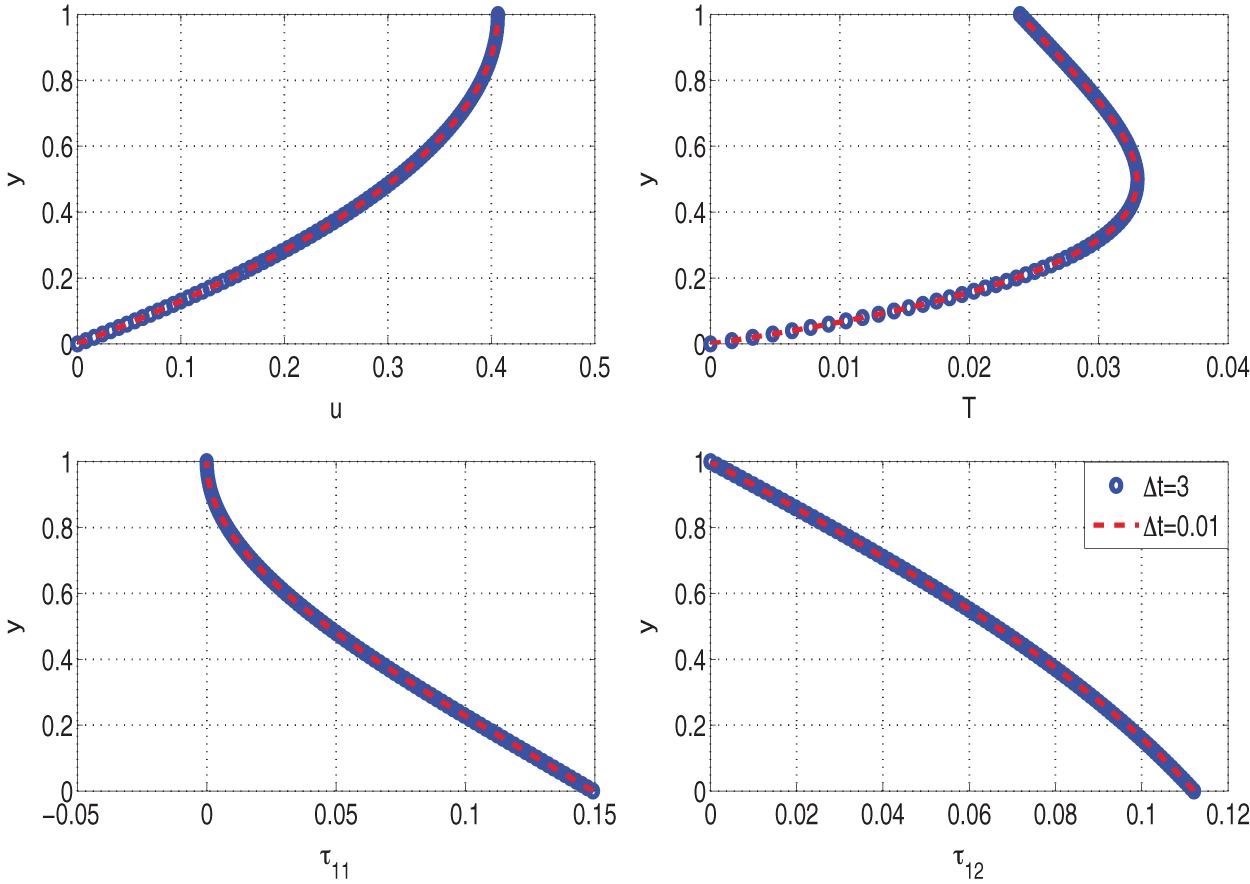
Figure 5: Time-step independence of solutions

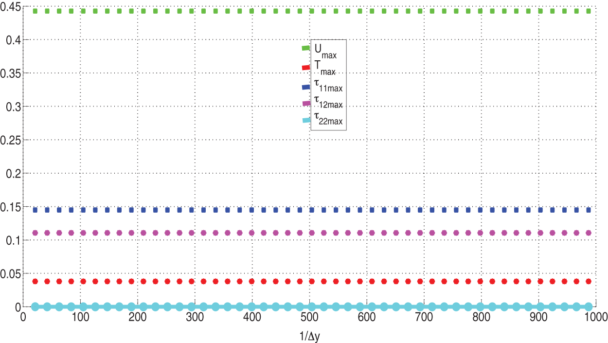
Figure 6: Mesh-size independence of maximum solutions

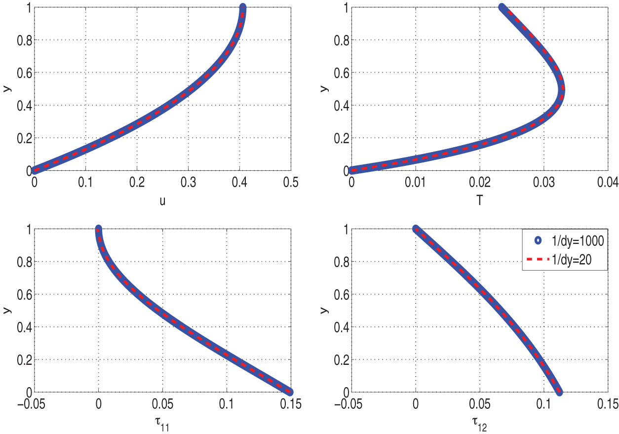
Figure 7: Mesh-size independence of solutions

4.3 Code Validation

A similar investigation to the current one was conducted in [29] using the Oldroyd-B constitutive model and in the absence of nanoparticles. The Oldroyd-B model is obtained from the Giesekus model by taking the nonlinear parameters as zero, i.e., ε=0 . The absence of nanoparticles in [29] mathematically reduces to taking φ=0 . The study in [29] therefore used the ordinary Oldroyd-B constitutive model with constant thermal-conductivity, κnf≡κf , i.e., κs=ℵ=A2=0 . By taking κs=0 , ℵ=0 , ε=0 , φ=0 , and A2=0 in the current model, the VFBN results reduce to those for a normal viscoelastic (Oldroyd-B) fluid and are exactly the same as those in [29].

4.4 Sensitivity of Solutions to Embedded Parameters

A representative sample of the flow behavior of field variables with variations in the fluid and flow parameters is now presented. The sensitivity of the VFBN thermal conductivity to changes in φ is illustrated in Fig. 8. As expected, the VFBN thermal-conductivity increases with increasing nanofluid volume-fraction, φ .

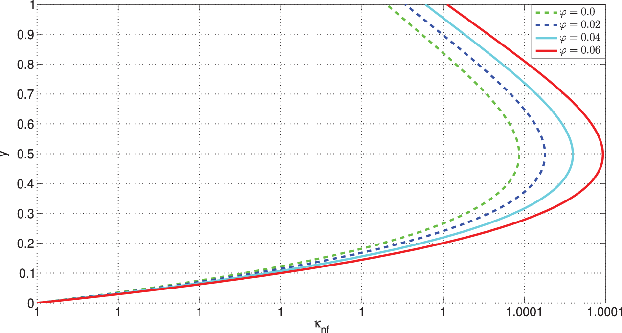
Figure 8: Variation of VFBN thermal conductivity with φ

It therefore naturally follows that the VFBN temperature increases with increasing φ . This expected response of the VFBN temperature to variations in φ is illustrated in Fig. 9. An increase in fluid temperature directly results in a reduction in fluid viscosity and hence an increase in the fluid velocity. It is therefore expected that the VFBN velocity would increase with increasing VFBN temperature. This expected increase of the VFBN velocity to variations in φ is also illustrated in Fig. 9. Lastly, Fig. 9 demonstrates an increase in the polymeric-stresses with increasing nanofluid volume-fraction, φ .

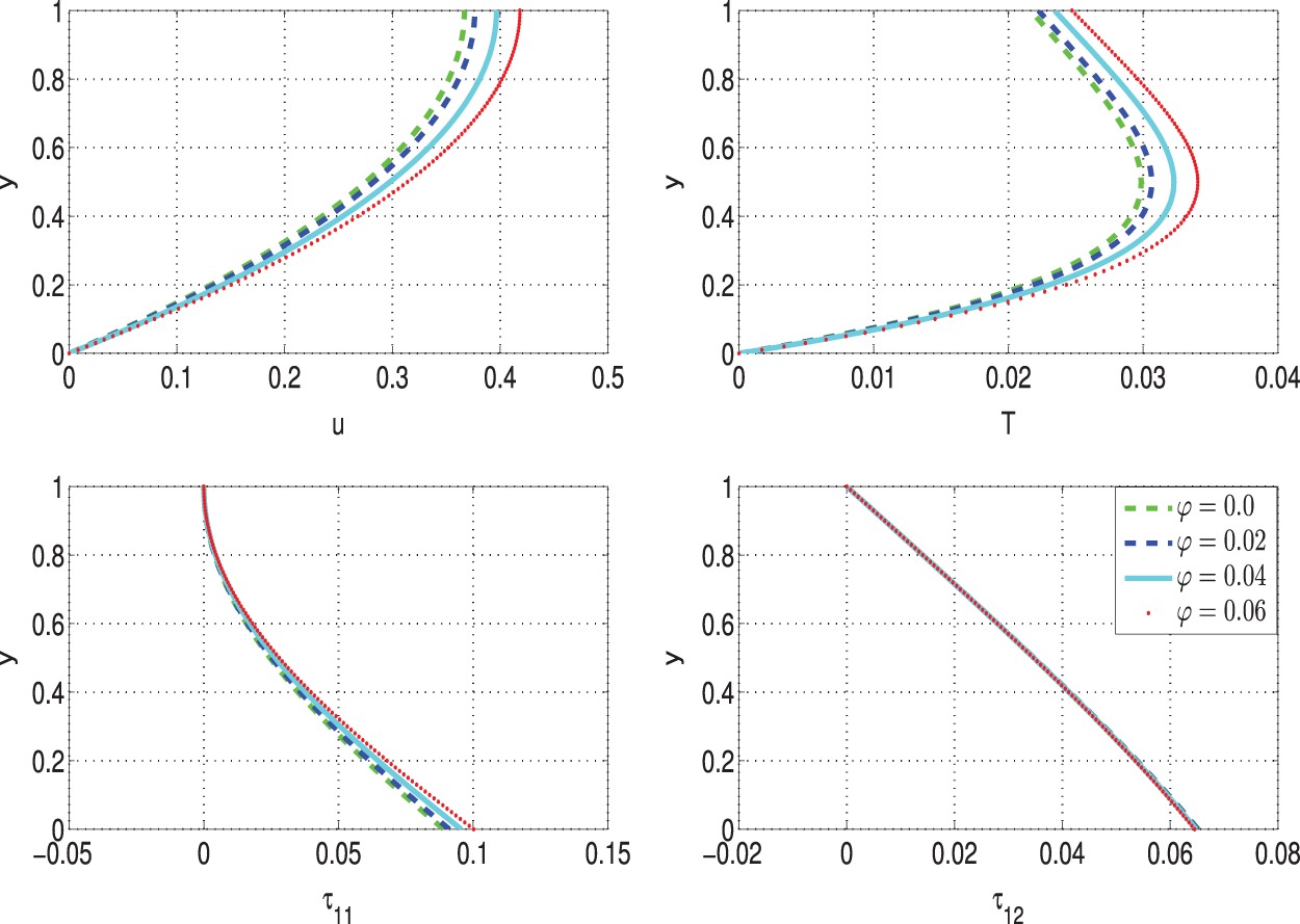
Figure 9: Variation of VFBN flow quantities with φ

Similar responses (as with φ ) of the VFBN thermal-conductivity to variations in both the thermal-conductivity parameter, A2 , and the activation-energy parameter, α , are respectively illustrated in Figs. 10 and 11.

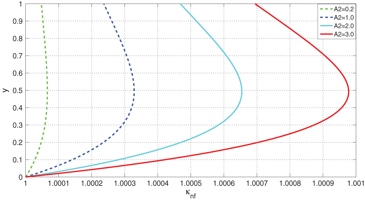
Figure 10: Variation of VFBN thermal conductivity with A2

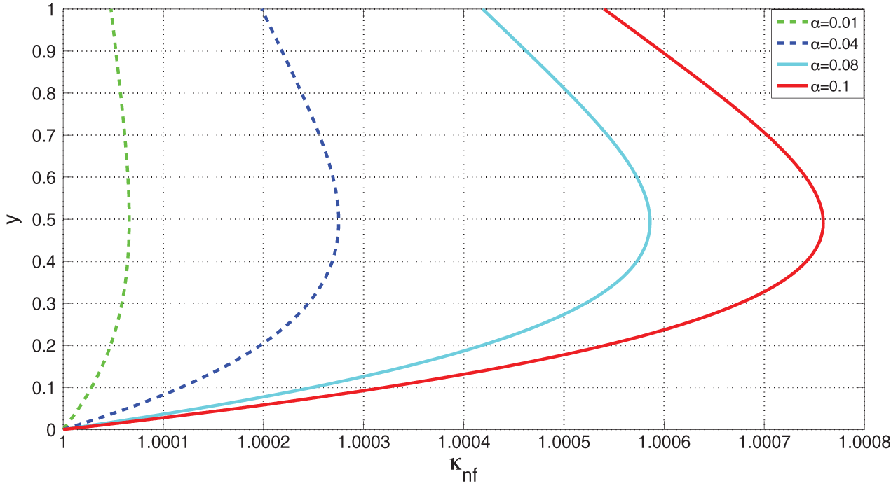
Figure 11: Variation of VFBN thermal conductivity with α

Fig. 12 shows the response of flow quantities to variations in the nanofluid Prandtl number, Prnf . Noting that Prnf is inversely proportional to the strength of the heat sources, the VFBN thermal conductivity (subsequently therefore the VFBN temperature) should decrease as Prnf increases. These expected results illustrated in Figs. 12 and 13, respectively.

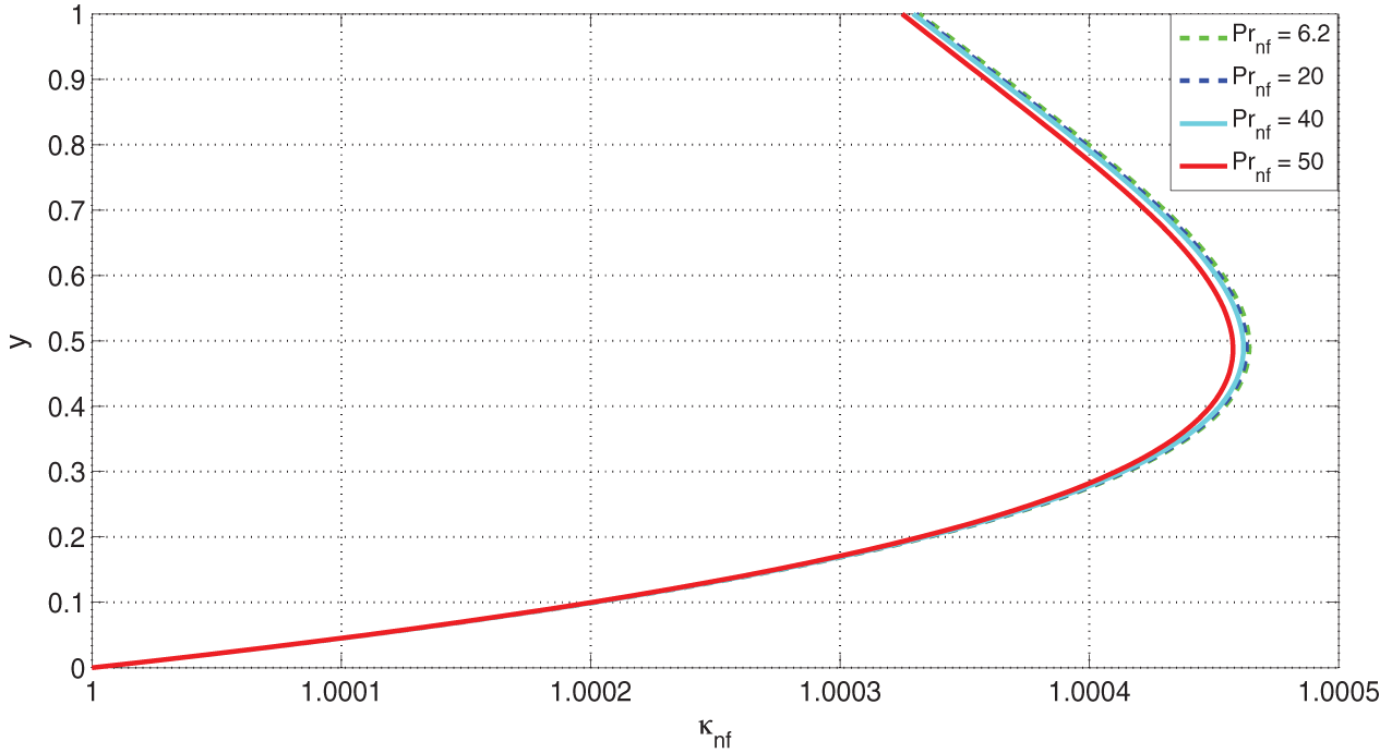
Figure 12: Effects of Prnf on VFBN thermal conductivity

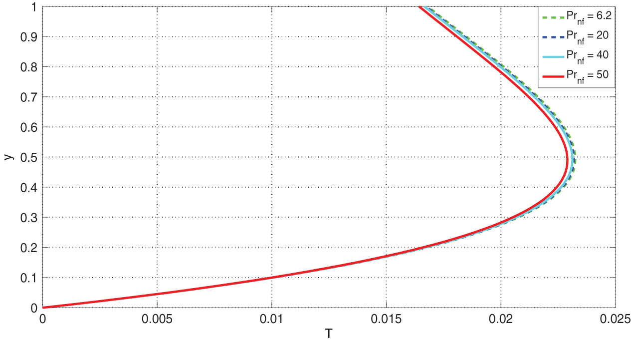
Figure 13: Effects of Prandtl Number, Prnf , on VFBN temperature

The behaviour of VFBN thermal conductivity with variations in the Deborah number, De, is illustrated in Fig. 14. It is observed that the VFBN thermal-conductivity increases with increasing De.

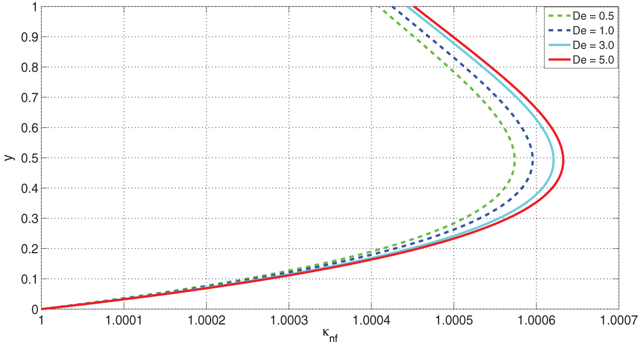
Figure 14: Effects of De on VFBN thermal conductivity

4.5 Wall Shear-Stress and Wall Heat Transfer Rate

As was already observed in the previous section, the nanofluid (VFBN) velocity and temperature both increase with increasing φ,Prnf , and De, see Figs. 8, 9, 12–14. The wall shear-stress and wall heat transfer rate (at the inclined wall) follow the same patterns, they both also increase with increasing φ,Prnf , and De.

5  Concluding Remarks

Efficient and robust computational and numerical schemes based on semi-implicit FDM were employed to investigate the thermo-physical and fluid-dynamical characteristics of a non-isothermal, free-surface, thin-film, gravity-driven flow of a VFBN. The VFBN flows down an inclined-plane and is subjected to convective-cooling at the fluid-air interface, i.e., the free-surface. The numerical and computational algorithms were checked for convergence in both space and time and were also positively validated against the results in the existing literature. A single-phase nanofluid model, in which metallic nanoparticles of spherical shape are homogenously mixed (ensuring non-sedimentation) to a viscoelastic base fluid of the Giesekus type, was adopted. The results illustrate that the volume-fraction of the embedded nanoparticles play fundamental roles in the fluid-dynamical and thermodynamical properties of the VFBN. Specifically, the VFBN thermal-conductivity, VFBN temperature, VFBN velocity, and VFBN polymeric stresses (in particular, the first normal stress difference) all increase as the nanoparticle volume-fraction increases. The results are of fundamental industrial significance and importance, especially to heating and cooling applications where heat-transfer-rate (HTR) enhancement and thermal-conductivity improvement may be achieved via nanoparticles and nanofluidics.

Funding Statement: The authors received no specific funding for this study.

Conflicts of Interests: The authors declare that they have no conflicts of interest to report regarding the present study.

References

1. Khan, I., Chinyoka, T., Gill, A. (2022). Dynamics of non-isothermal pressure-driven flow of generalized viscoelastic-fluid-based nanofluids in a channel. Mathematical Problems in Engineering, 2022, 9080009. DOI 10.1155/2022/9080009. [Google Scholar] [CrossRef]
2. Khan, I., Chinyoka, T., Gill, A. (2022). Computational analysis of shear banding in simple shear flow of viscoelastic fluid-based nanofluids subject to exothermic reactions. Energies, 15(5), 1719. DOI 10.3390/en15051719. [Google Scholar] [CrossRef]
3. Khan, I., Chinyoka, T., Gill, A. (2022). Computational analysis of the dynamics of generalized-viscoelastic-fluid-based nanofluids subject to exothermic-reaction in shear-flow. Journal of Nanofluids, 11(4), 487–499. [Google Scholar]
4. Sheikhpour, M., Arabi, M., Kasaeian, A., Rokn Rabei, A., Taherian, Z. (2020). Role of nanofluids in drug delivery and biomedical technology: Methods and applications. Nanotechnology, Science and Applications, 13, 47–59. [Google Scholar]
5. Wong, K. V., de Leon, O. (2017). Applications of nanofluids: Current and future. In: Nanotechnology and energy, pp. 105–132. Jenny Stanford Publishing. [Google Scholar]
6. Li, F. C., Yang, J. C., Zhou, W. W., He, Y. R., Huang, Y. M. et al. (2013). Experimental study on the characteristics of thermal conductivity and shear viscosity of viscoelastic-fluid-based nanofluids containing multiwalled carbon nanotubes. Thermochimica Acta, 556, 47–53. DOI 10.1016/j.tca.2013.01.023. [Google Scholar] [CrossRef]
7. Sundar, L. S., Naik, M. T., Sharma, K. V., Singh, M. K., Reddy, T. C. S. (2012). Experimental investigation of forced convection heat transfer and friction factor in a tube with Fe3O4 magnetic nanofluid. Experimental Thermal and Fluid Science, 37, 65–71. DOI 10.1016/j.expthermflusci.2011.10.004. [Google Scholar] [CrossRef]
8. Yang, J. C., Li, F. C., Zhou, W. W., He, Y. R., Jiang, B. C. (2012). Experimental investigation on the thermal conductivity and shear viscosity of viscoelastic-fluid-based nanofluids. International Journal of Heat and Mass Transfer, 55(11–12), 3160–3166. DOI 10.1016/j.ijheatmasstransfer.2012.02.052. [Google Scholar] [CrossRef]
9. Sajadi, A. R., Kazemi, M. H. (2011). Investigation of turbulent convective heat transfer and pressure drop of TiO2/water nanofluid in circular tube. International Communications in Heat and Mass Transfer, 38(10), 1474–1478. DOI 10.1016/j.icheatmasstransfer.2011.07.007. [Google Scholar] [CrossRef]
10. Kleinstreuer, C., Feng, Y. (2011). Experimental and theoretical studies of nanofluid thermal conductivity enhancement: A review. Nanoscale Research Letters, 6(1), 1–13. [Google Scholar]
11. Kalteh, M., Abbassi, A., Saffar-Avval, M., Harting, J. (2011). Eulerian-eulerian two-phase numerical simulation of nanofluid laminar forced convection in a microchannel. International Journal of Heat and Fluid Flow, 32(1), 107–116. [Google Scholar]
12. Kondaraju, S., Jin, E. K., Lee, J. S. (2010). Investigation of heat transfer in turbulent nanofluids using direct numerical simulations. Physical Review E, 81(1), 016304. DOI 10.1103/PhysRevE.81.016304. [Google Scholar] [CrossRef]
13. Özerinç, S., Kakaç, S., Yazcoğlu, A. G. (2010). Enhanced thermal conductivity of nanofluids: A state-of-the-art review. Microfluidics and Nanofluidics, 8(2), 145–170. [Google Scholar]
14. Terekhov, V. I., Kalinina, S. V., Lemanov, V. V. (2010). The mechanism of heat transfer in nanofluids: State of the art (review). Part 1, synthesis and properties of nanofluids. Thermophysics and Aeromechanics, 17(1), 1–14. DOI 10.1134/S0869864310010014. [Google Scholar] [CrossRef]
15. Chandrasekar, M., Suresh, S. (2009). Determination of heat transport mechanism in aqueous nanofluids using regime diagram. Chinese Physics Letters, 26(12), 124401. DOI 10.1088/0256-307X/26/12/124401. [Google Scholar] [CrossRef]
16. Behzadmehr, A., Saffar-Avval, M., Galanis, N. (2007). Prediction of turbulent forced convection of a nanofluid in a tube with uniform heat flux using a two phase approach. International Journal of Heat and Fluid Flow, 28(2), 211–219. DOI 10.1016/j.ijheatfluidflow.2006.04.006. [Google Scholar] [CrossRef]
17. Zhou, X. F., Gao, L. (2007). Effect of multipolar interaction on the effective thermal conductivity of nanofluids. Chinese Physics, 16(7), 2028. DOI 10.1088/1009-1963/16/7/037. [Google Scholar] [CrossRef]
18. Maiga, S. E. B., Palm, S. J., Nguyen, C. T., Roy, G., Galanis, N. (2005). Heat transfer enhancement by using nanofluids in forced convection flows. International Journal of Heat and Fluid Flow, 26(4), 530–546. [Google Scholar]
19. Roy, G., Nguyen, C. T., Lajoie, P. R. (2004). Numerical investigation of laminar flow and heat transfer in a radial flow cooling system with the use of nanofluids. Superlattices and Microstructures, 35(3–6), 497–511. DOI 10.1016/j.spmi.2003.09.011. [Google Scholar] [CrossRef]
20. Xuan, Y., Li, Q. (2003). Investigation on convective heat transfer and flow features of nanofluids. Journal of Heat Transfer, 125(1), 151–155. DOI 10.1115/1.1532008. [Google Scholar] [CrossRef]
21. Keblinski, P., Phillpot, S. R., Choi, S. U., Eastman, J. A. (2002). Mechanisms of heat flow in suspensions of nano-sized particles (nanofluids). International Journal of Heat and Mass Transfer, 45(4), 855–863. DOI 10.1016/S0017-9310(01)00175-2. [Google Scholar] [CrossRef]
22. Eastman, J. A., Choi, S. U., Li, S., Yu, W., Thompson, L. J. (2001). Anomalously increased effective thermal conductivities of ethylene glycol-based nanofluids containing copper nanoparticles. Applied Physics Letters, 78(6), 718–720. DOI 10.1063/1.1341218. [Google Scholar] [CrossRef]
23. Xuan, Y., Li, Q. (2000). Heat transfer enhancement of nanofluids. International Journal of Heat and Fluid Flow, 21(1), 58–64. [Google Scholar]
24. Li, S., Eastman, J. A. (1999). Measuring thermal conductivity of fluids containing oxide nanoparticles. Journal of Heat Transfer, 121(2), 280–289. DOI 10.1115/1.2825978. [Google Scholar] [CrossRef]
25. Chinyoka, T. (2021). Comparative response of Newtonian and non-Newtonian fluids subjected to exothermic reactions in shear flow. International Journal of Applied and Computational Mathematics, 7(3), 1–19. DOI 10.1007/s40819-021-01023-4. [Google Scholar] [CrossRef]
26. Abuga, J. G., Chinyoka, T. (2020). Benchmark solutions of the stabilized computations of flows of fluids governed by the rolie-poly constitutive model. Journal of Physics Communications, 4(1), 015024. DOI 10.1088/2399-6528/ab6ed2. [Google Scholar] [CrossRef]
27. Abuga, J. G., Chinyoka, T. (2020). Numerical study of shear banding in flows of fluids governed by the rolie-poly two-fluid model via stabilized finite volume methods. Journal of Physics Communications, Processes, 8(7), 810. DOI 10.3390/pr8070810. [Google Scholar] [CrossRef]
28. Ireka, I. E., Chinyoka, T. (2016). Analysis of shear banding phenomena in non-isothermal flow of fluids governed by the diffusive Johnson-Segalman model. Applied Mathematical Modelling, 40(5–6), 3843–3859. DOI 10.1016/j.apm.2015.11.005. [Google Scholar] [CrossRef]
29. Chinyoka, T., Goqo, S. P., Olajuwon, B. I. (2013). Computational analysis of gravity driven flow of a variable viscosity viscoelastic fluid down an inclined plane. Computers & Fluids, 84, 315–326. DOI 10.1016/j.compfluid.2013.06.022. [Google Scholar] [CrossRef]
30. Chinyoka, T. (2010). Poiseuille flow of reactive phan-thien-tanner liquids in 1D channel flow. Journal of Heat Transfer, 132(11), 111701. DOI 10.1115/1.4002094. [Google Scholar] [CrossRef]
31. Chinyoka, T. (2009). Viscoelastic effects in double pipe single pass counterflow heat exchangers. International Journal for Numerical Methods in Fluids, 59(6), 677–690. DOI 10.1002/fld.1839. [Google Scholar] [CrossRef]
32. Chinyoka, T. (2009). Modeling of cross-flow heat exchangers with viscoelastic fluids. Nonlinear Analysis: Real World Applications, 10(6), 3353–3359. DOI 10.1016/j.nonrwa.2008.10.069. [Google Scholar] [CrossRef]
33. Chinyoka, T. (2008). Computational dynamics of a thermally decomposable viscoelastic lubricant under shear. Journal of Fluids Engineering, 130(12), 121201. DOI 10.1115/1.2978993. [Google Scholar] [CrossRef]
34. Chinyoka, T. (2004). Numerical simulation of stratified flows and droplet deformation in 2D shear flow of Newtonian and viscoelastic fluids (Ph.D. Thesis). Virginia Tech. [Google Scholar]
35. Khan, M., Lone, S. A., Rasheed, A., Alam, M. N. (2022). Computational simulation of scott-blair model to fractional hybrid nanofluid with darcy medium. International Communications in Heat and Mass Transfer, 130, 105784. DOI 10.1016/j.icheatmasstransfer.2021.105784. [Google Scholar] [CrossRef]
36. Khan, M., Rasheed, A. (2021). A numerical study of hybrid nanofluids near an irregular 3D surface having slips and exothermic effects. Proceedings of the Institution of Mechanical Engineers, Part E: Journal of Process Mechanical Engineering, 236(4), 1273–1282. DOI 10.1177/09544089211064761. [Google Scholar] [CrossRef]
37. Khan, M., Rasheed, A. (2022). Numerical implementation and error analysis of nonlinear coupled fractional viscoelastic fluid model with variable heat flux. Ain Shams Engineering Journal, 13(3), 101614. DOI 10.1016/j.asej.2021.10.009. [Google Scholar] [CrossRef]
38. Khan, M., Rasheed, A. (2021). Scott-blair model with unequal diffusivities of chemical species through a Forchheimer medium. Journal of Molecular Liquids, 341, 117351. DOI 10.1016/j.molliq.2021.117351. [Google Scholar] [CrossRef]
39. Khan, M., Rasheed, A. (2021). Computational analysis of heat transfer intensification of fractional viscoelastic hybrid nanofluids. Mathematical Problems in Engineering, 2021, 2544817. [Google Scholar]
40. Ghadikolaei, S. S., Hosseinzadeh, K., Ganji, D. D., Jafari, B. (2018). Nonlinear thermal radiation effect on magneto Casson nanofluid flow with joule heating effect over an inclined porous stretching sheet. Case Studies in Thermal Engineering, 12, 176–187. DOI 10.1016/j.csite.2018.04.009. [Google Scholar] [CrossRef]
41. Usman, M., Soomro, F., Haq, R., Wang, W., Defterli, O. (2018). Thermal and velocity slip effects on Casson nanofluid flow over an inclined permeable stretching cylinder via collocation method. International Journal of Heat and Mass Transfer, 122, 1255–1263. DOI 10.1016/j.ijheatmasstransfer.2018.02.045. [Google Scholar] [CrossRef]
42. Chen, L., Wang, Y., Qi, C., Tang, Z., Tian, Z. (2022). A review of methods based on nanofluids and biomimetic structures for the optimization of heat transfer in electronic devices. Fluid Dynamics & Materials Processing, 18(5), 1205–1227. DOI 10.32604/fdmp.2022.021200. [Google Scholar] [CrossRef]
43. Kuzmenkov, D., Struchalin, P., Litvintsova, Y., Delov, M., Skrytnyy, V. et al. (2022). Influence of particle size distribution on the optical properties of fine-dispersed suspensions. Fluid Dynamics & Materials Processing, 18(1), 1–14. DOI 10.32604/fdmp.2022.018526. [Google Scholar] [CrossRef]
44. Abdeljawad, T., Riaz, M. B., Saeed, S. T., Iftikhar, N. (2021). MHD Maxwell fluid with heat transfer analysis under ramp velocity and ramp temperature subject to non-integer differentiable operators. Computer Modeling in Engineering & Sciences, 126(2), 821–841. DOI 10.32604/cmes.2021.012529. [Google Scholar] [CrossRef]
Cite This Article
Copyright © 2023 The Author(s). Published by Tech Science Press.
This work is licensed under a Creative Commons Attribution 4.0 International License , which permits unrestricted use, distribution, and reproduction in any medium, provided the original work is properly cited.
Downloads
Citation Tools