
 Submit a Paper
 Propose a Special lssue
 Open Access
ARTICLE

Unsteady Heat Transfer in Bilayer, and Three-Layer Materials
1 Physics Department, Faculty of Sciences, University of Saida Dr. Moulay Tahar, Saida, 20000, Algeria
2 Theoretical Physics Laboratory, University of Oran -1- Ahmed Ben Bella, Oran, 31000, Algeria
* Corresponding Author: Toufik Sahabi. Email:
(This article belongs to the Special Issue: Materials and Energy an Updated Image for 2021)
Fluid Dynamics & Materials Processing 2023, 19(4), 977-990. https://doi.org/10.32604/fdmp.2022.022059
Received 18 February 2022; Accepted 21 June 2022; Issue published 02 November 2022
 View Full Text
 Download PDF
Abstract
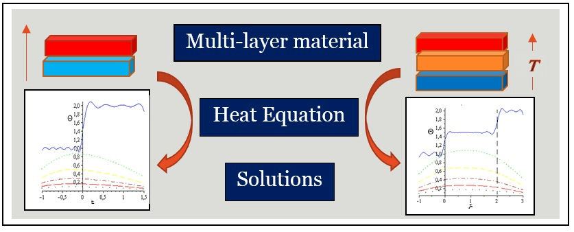
The heat transfer equation is used to determine the heat flow by conduction through a composite material along the real axis. An analytical dimensionless analysis is implemented in the framework of a separation of variables method (SVM). This approach leads to an Eigenvalues problem that is solved by the Newton’s method. Two types of dynamics are found: An unsteady condition (in the form of jumps or drops in temperatures depending on the considered case), and a permanent equilibrium (tending to the ambient temperature). The validity and effectiveness of the proposed approach for any number of adjacent layers is also discussed. It is shown that, as expected, the diffusion of the temperature is linked to the ratio of the thermo-physical properties of the considered layers and their number.Graphic Abstract
Keywords
Nomenclature
| i | Layer’s index ( |
| | Layer’s temperature [K] |
| | Ambient temperature [K] |
| | Initial temperature in ith layer [K] |
| | Initial deference in temperatures [K] |
| | Deference in temperatures [K] |
| | Layer’s thickness [m] |
| | Conductivity [W.m−1.K−1] |
| | Diffusivity [m2.s−1] |
| | Specific heat [J.Kg−1.K−1] |
| | Density [Kg.m−3] |
| | Convection coefficient [W.m−2.K−1] |
| | Dimensionless diffusivity |
| | Dimensionless conductivity |
| | Dimensionless thickness |
| | Biot numbers |
| | Dimensionless Eigen-values |
| | Dimensionless time |
| | Dimensionless position |
| | Dimensionless initial, temporal and unsteady equilibrium temperatures respectively |
The heat equation, describing heat transfer by conduction, is a partial differential equation, established by J. Fourier in the end of the 19th century after certain experiments. It has a great interest in mathematics and physics. This transfer can be studied either in a single body or through several systems with different thermo-physical properties. In the literature, there are several interesting works, based on certain original references [1]. The research is varied according to the interests of the authors, such as the fractional order heat equation in higher space-Time dimensions [2], its numerical resolution [3], and application for heat spreading of electronic components [4]. For numerical resolution of heat equation in various conditions, Local least–squares element differential method is used to solve heat conduction problems in composite structures [5]. Recently, regarding the problems of realization on the site related to the use of heat sources as well as the optimization of energy consumption, a one-dimensional model is used by Tlili et al. [6] to research the belongings of different functional and geometrical parameters on energy consumption of flat distance direct contact membrane distillation (DCMD) for solar desalination tasks. Furthermore, to reduce the energy consumption in the fresh water production, using the solar energy, the same model is utilized to examine the effect of dissimilar operational and geometrical parameters on energy consumption of flat sheet DCMD for solar desalination purposes [7].
In our paper, the transfer problem by conduction across bilayer and three-layer materials is investigated, adopting the same notations, as used in [8], with some small modifications. Firstly, the separation of variables method (SVM) is used to solve the two heat equations in the two slabs with the associated boundary and initial conditions. The total procedure is well detailed in [9,10], showing how to obtain the so-called Eigen-problem whose dimensionless solutions called roots, are used to give the explicit form of the heat transfer. Then, using orthogonal properties between the two space solutions, we get the integral constants, and thus, the final form of the solutions. Subsequently, according to the material’s thermo-physical properties [11], the transfer heat change is explained. The influence of these properties on the heat transfer between the two layers materials is described. In the three-layer case, a new coupling function
We consider a material composed of two different regions
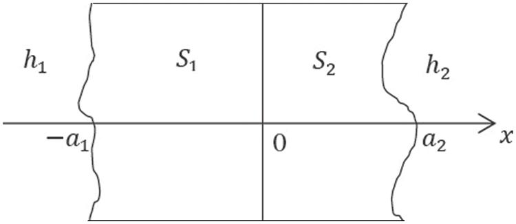
Figure 1: Representation of bilayer material
where,
The one-dimensional heat conduction without thermal source for the two slabs, is given by [1]
with the set of boundary conditions (BCs) [8] at the edges
and on the contact surface, we have
The initial conditions (ICs), for each layer, are supposed constants
We have now, a full solvable system constructed by Eqs. (2)–(7). The analytic solutions are
For each layer, the solutions are obtained easily by SVM, where
Dimensionless calculus has been used for several reasons and purposes. We are talking about: The simplicity of the calculations, the reduction of the parameters, the permanent verification of the homogeneity of the equations, the writing of the formulas will be more compact and more significant as well as the ease of reading the curves because the intervals of variations of the solution temperatures are reduced to acute and positive intervals. Then, the dimensionless group is defined by [10].
and the Biot numbers
Then, after some manipulations (see [12] for full detail), we can reduce our problem to the determination of the constants
called Eigen values, representing the non-vanishing dimensionless roots of the function
With
We reconstruct our solutions under the dimensionless form, as
where, we introduce the space-time dimensionless coordinates:
The determination of
An order higher than 20 roots can be reached, having a small influence on the result (see Section 4.1). We note that initially, there is an unsteady equilibrium temperature between the two slabs. It is analytically given by [12]
where,
where, the dimensionless initial temperatures
The error is defined as the relative difference, at zero time, between calculated temperature, obtained by Eq. (22), and our initial conditions (
As can be seen,
The same reasoning can be used, for the case of three-layer material. We consider a material composed of three different regions
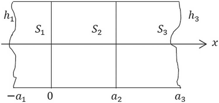
Figure 2: Representation of three-layer material
with
where,
Thus, the temporal and space solutions take, according to the Eigen values set
The final dimensionless solution is expanded as a linear combination of products of the temporal and space parts
We can regroup, similarly as Eq. (22), the three temperatures in a single expression, describing the whole material as
Note that the unsteady equilibrium temperature, between any two adjacent slabs i, i+1 (
The final dimensionless solution is expanded as a linear combination of products of the temporal and space parts. Therefore, the dimensionless unsteady equilibrium temperature is
The error is defined by
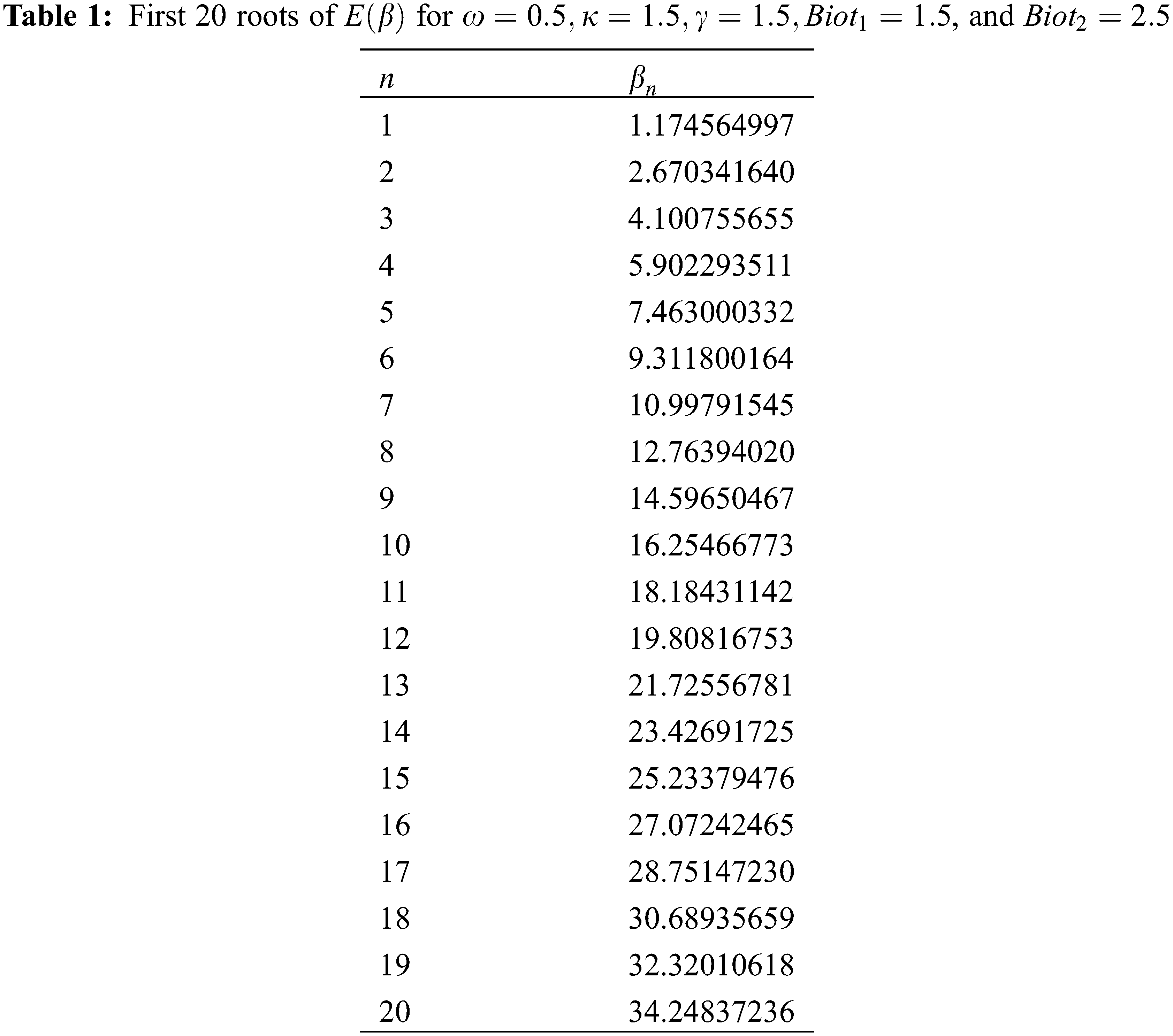
By taking the instance, presented in Table 1, and for
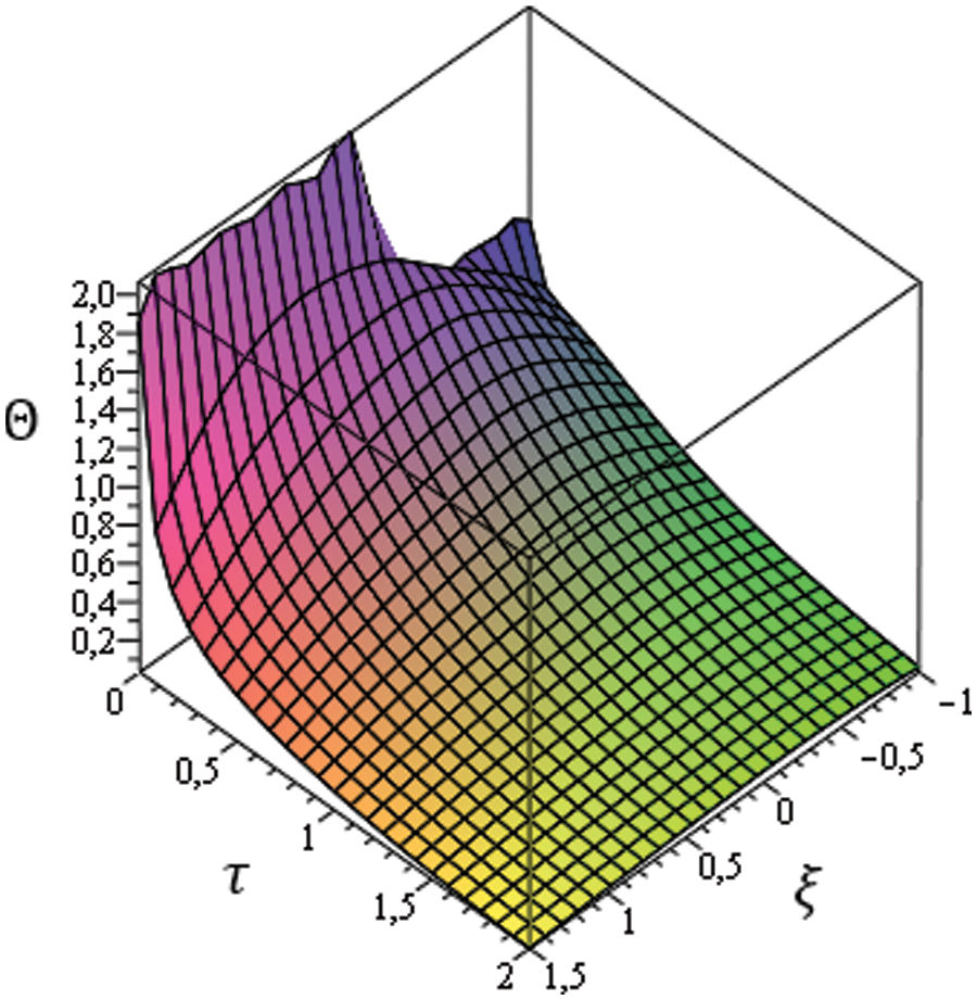
Figure 3: 3D representation of temperature evolution in bilayer material
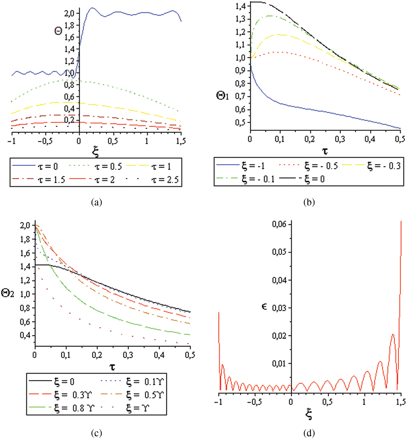
Figure 4: Temperature curves; (a): With respect to the position in different times, (b): For S1, in different positions in the first moments, (c): For S2, in different positions in the first moments, (d): The error with respect to the position for equal ICs
Figs. 4b and 4c represent the temperature in term of time at selected points, in both layers. From Fig. 4b, the unsteady equilibrium can clearly be seen.
To reach that, in the first layer, the temperature increases, proportionally to the distance from the contact surface, with small values, called temperature jumps, while the taken time is inversely proportional to this distance. Hence, the final thermal equilibrium is achieved. For the second layer, the temperature converges to the equilibrium one, with a much slower pace, due to its thickness that is greater than that of the first layer.
We also emphasize that the unsteady equilibrium is clear, for
The heat transfer, in bilayer material, is well described according to thermo-physical properties (Eqs. (11)–(14)) of the two layers (cf. Section 2). For equal ICs, (from full Maple procedure) its behavior is presented according to the number of roots in the solution, and parameter, keeping the others constants (Fig. 5). This parametric study consists in fixing a thermo-physical property such as the conductivity, and diffusivity, of the first layer with changing that of the other [12,13].
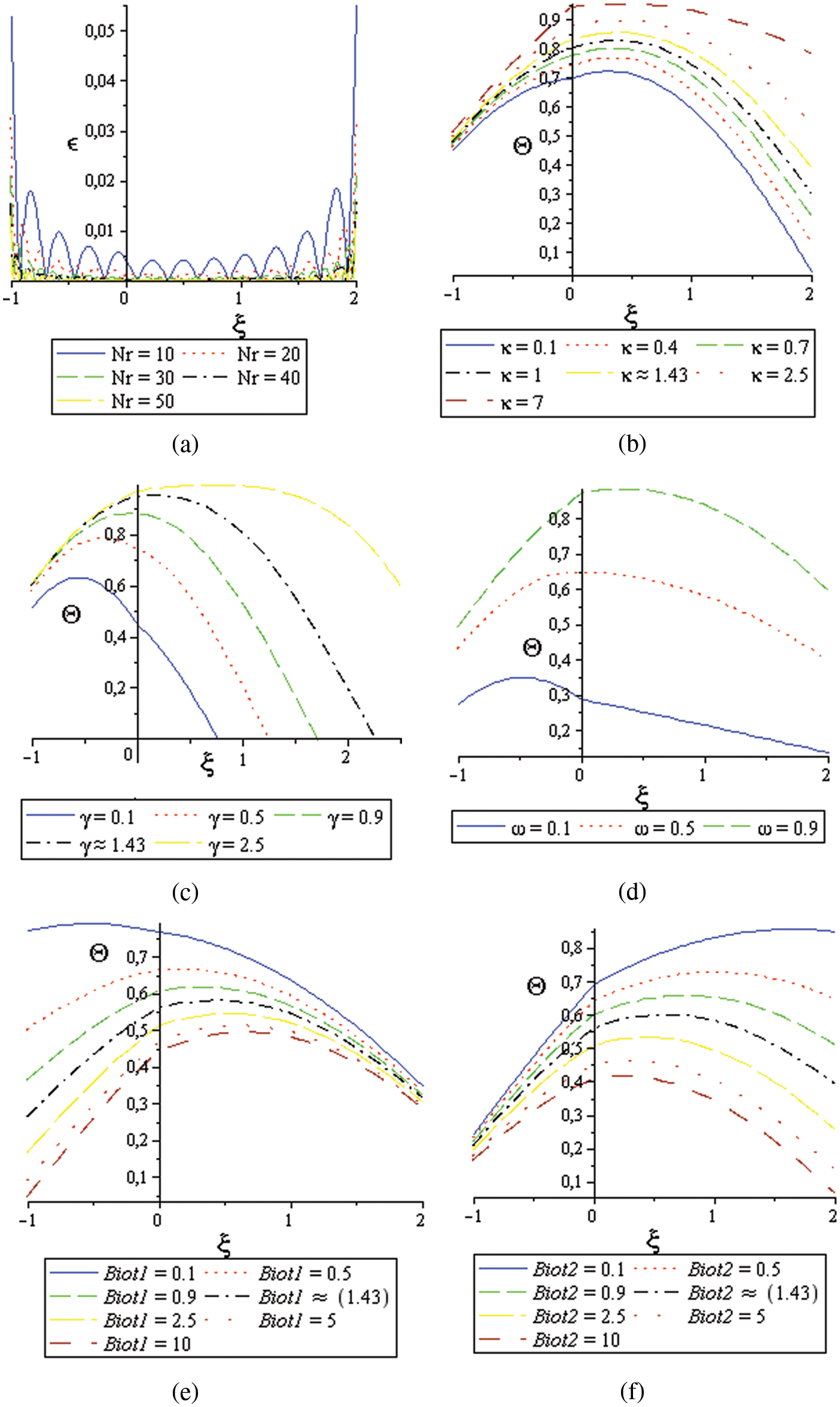
Figure 5: Parametric study; (a): Error according to the number of the roots
The error with respect to the number of roots
Similarly, one can observe the same reaction of heat transfer vs. the thickness report
In this case, we consider the example where
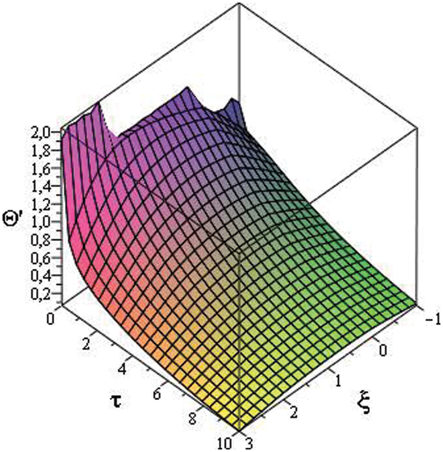
Figure 6: 3D representation of temperature evolution in three-layer material
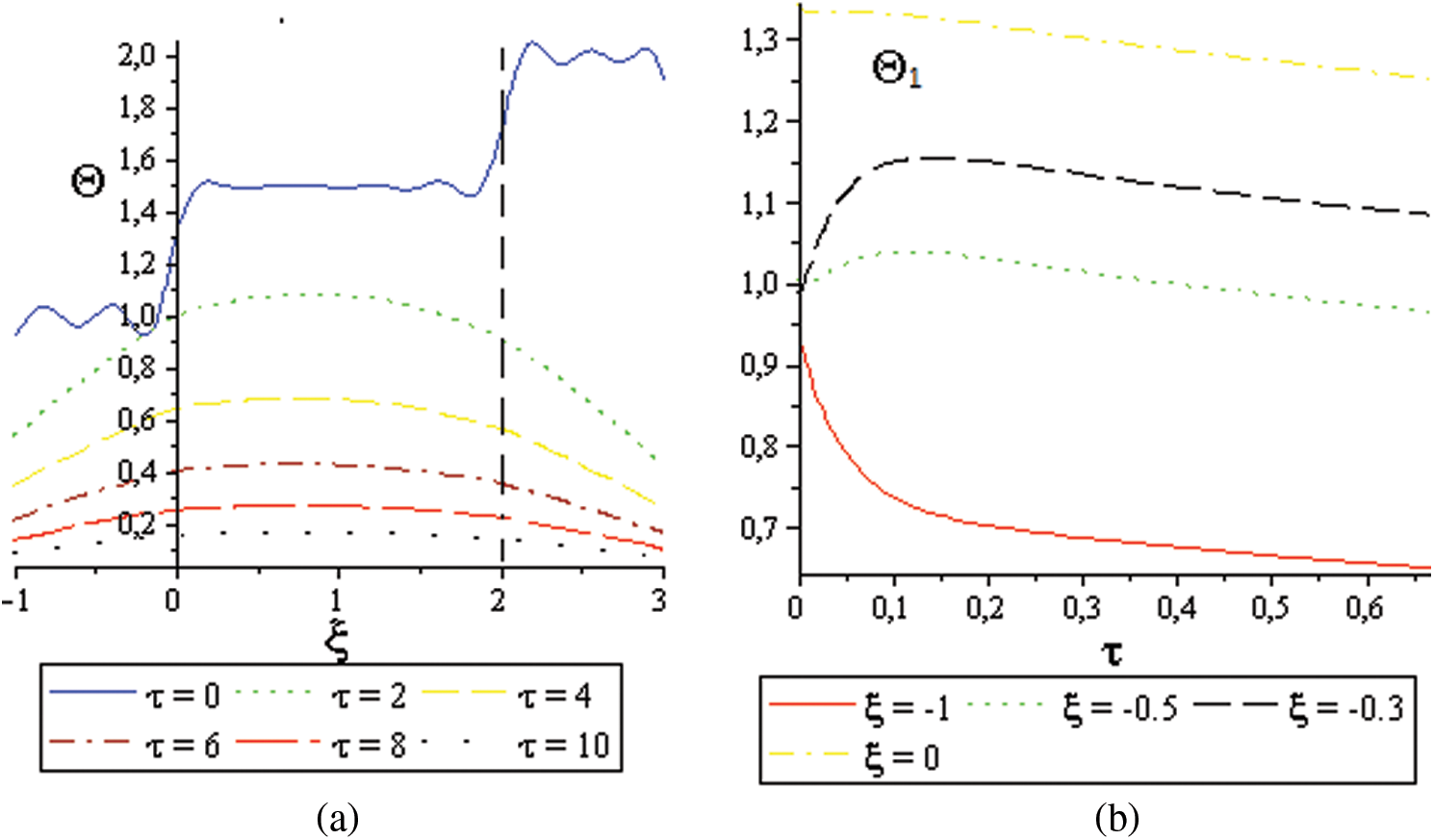
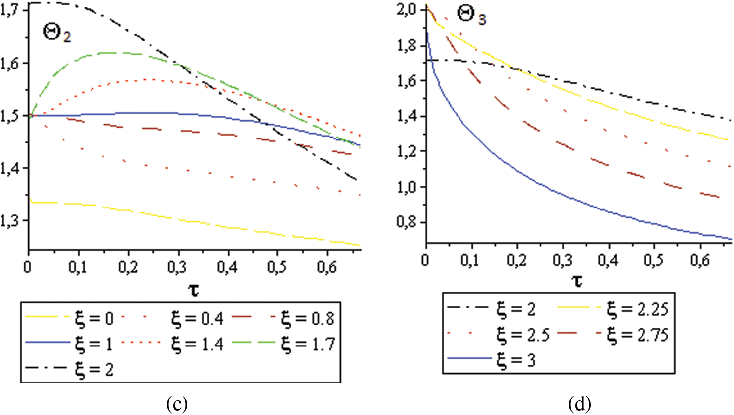
Figure 7: Temperature’s behavior in three-layer material: (a) Heat transient in different times, (b) Heat behavior in the first layer at the first moments in different points, (c) Heat behavior in the second layer in different points at the first moments, (d) Heat behavior in the third layer in different points at the first moments
Fig. 7a shows, in the first moments, the heat transit at
The continuity of
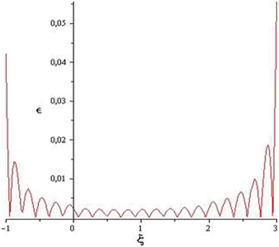
Figure 8: Error with respect to the position for a three-layer material
The divergence of the graphs in the boundaries (
This analytical study shows that there is a similarity in the evolution of heat transfer between two layers as well as between three layers. In both cases, we note that an unsteady thermal equilibrium occurs moments before the final thermal equilibrium. Mathematically, we notice that we get the same form for the solutions, except for the coupling function
Concerning the accuracy of the results, this is based on two points having almost significant equivalence: The first is the exact analytical calculation by SVM and using the Maple Program, which brings us back to the similar results detailed in the literature. The second point is the concordance with the experimental prediction, which explains the existence of two kinds of equilibrium: Unsteady, and permanent similar to the damped movement in the mechanical vibration of solids or fluids (Transitional and permanent diverge).
Acknowledgement: T. Sahabi would like to thank Prof. F. de Monte for his assistance in this research in terms of providing references and answering questions, and Prof. Mohamed El Ganaoui for his encouragement and providing references.
Funding Statement: The authors received no specific funding for this study.
Conflicts of Interest: The authors declare that they have no conflicts of interest to report regarding the present study.
References
1. Carslaw, H. S., Jaeger, J. C. (1959). Conduction of heat in solids. England: Oxford University Press. [Google Scholar]
2. Singh, D., Tiwari, B. N., Yadav, N. (2017). Fractional order heat equation in higher space-time dimensions. https://arxiv.org/abs/1704.04101#. [Google Scholar]
3. Filipov, S., Faragó, I. (2018). Implicit Euler time discretization and FDM with Newton method in non-linear heat transfer modeling. International Scientific Journal, Mathematical Modeling, 2, 94–98. DOI 10.48550/arXiv.1811.06337. [Google Scholar] [CrossRef]
4. Samia, S., Dmitri, K., Alexander, A. B. (2009). Graphene heat spreaders for thermal management of nano-electronic circuits. DOI 10.48550/arXiv.0910.1883. [Google Scholar] [CrossRef]
5. Gao, X. W., Zheng, Y. T., Fantuzzi, N. (2020). Local least-squares element differential method for solving heat conduction problems in composite structures. Numerical Heat Transfer, Part B: Fundamentals, 77(6), 441–460. DOI 10.1080/10407790.2020.1746584. [Google Scholar] [CrossRef]
6. Tlili, I., Sajadi, S. M., Baleanu, D., Ghaemi, F. (2022). Flat sheet direct contact membrane distillation study to decrease the energy demand for solar desalination purposes. Sustainable Energy Technologies and Assessments, 52, 102100. DOI 10.1016/j.seta.2022.102100. [Google Scholar] [CrossRef]
7. Zhang, J., Sajadi, S. M., Chen, Y., Tlili, I., Fagiry, M. A. (2022). Effects of Al2O3 and TiO2 nanoparticles in order to reduce the energy demand in the conventional buildings by integrating the solar collectors and phase change materials. Sustainable Energy Technologies and Assessments, 52, 102114. DOI 10.1016/j.seta.2022.102114. [Google Scholar] [CrossRef]
8. de Monte, F. (2000). Transient heat conduction in one-dimensional composite slab. A ‘natural’ analytic approach. International Journal of Heat and Mass Transfer, 43(19), 3607–3619. DOI 10.1016/S0017-9310(00)00008-9. [Google Scholar] [CrossRef]
9. de Monte, F. (2002). An analytic approach to the unsteady heat conduction processes in one-dimensional composite media. International Journal of Heat and Mass Transfer, 45(6), 1333–1343. DOI 10.1016/S0017-9310(01)00226-5. [Google Scholar] [CrossRef]
10. de Monte, F. (2003). Unsteady heat conduction in two-dimensional two slab-shaped regions. Exact closed-form solution and results. International Journal of Heat and Mass Transfer, 46(8), 1455–1469. DOI 10.1016/S0017-9310(02)00417-9. [Google Scholar] [CrossRef]
11. Grimvall, G. (1999). Thermo-physical properties of materials. North Holland: Elsevier. [Google Scholar]
12. Belghazi, H. (2008). Modélisation analytique du transfert instationnaire de la chaleur dans un matériau bicouche en contact imparfait et soumis à une source de chaleur en mouvement (Ph.D. Thesis). France: University of Limoges. [Google Scholar]
13. Belghazi, H., El Ganaoui, M., Labbe, J. C. (2010). Analytical solution of unsteady heat conduction in a two-layered material in imperfect contact subjected to a moving heat source. International Journal of Thermal Sciences, 49(2), 311–318. DOI 10.1016/j.ijthermalsci.2009.06.006. [Google Scholar] [CrossRef]
Cite This Article
 Copyright © 2023 The Author(s). Published by Tech Science Press.
This work is licensed under a Creative Commons Attribution 4.0 International License , which permits unrestricted use, distribution, and reproduction in any medium, provided the original work is properly cited.
 Downloads
 Citation Tools