Thermal Properties Reconstruction and Temperature Fields in Asphalt Pavements: Inverse Problem and Optimisation Algorithms

1  Introduction

As two important factors to be considered in the design of asphalt pavement structure, high temperature stability [1–3] and low temperature crack resistance [4,5] are closely related to the temperature of asphalt pavement [6–8]. It is very important to study the distribution characteristics and change rules of the asphalt pavement temperature field. Road designers can determine the high-temperature stability performance and low-temperature crack resistance performance requirements of asphalt pavement according to different environmental parameters, make the selected pavement materials and structural parameters meet the design requirements. Moreover, Researchers can more easily analyze the mechanism of pavement diseases [9–11], and predict the temperature field of pavement structure according to the change of environmental conditions [12]. These are helpful in predicting the possible quality problems and diseases of the road structure and provide reference for the daily maintenance and quality safety assessment of the road.

Christison et al. [13] conducted continuous temperature monitoring on four different types of asphalt pavements in western Canada. The authors elaborated a linear relational expression between temperature parameters and air temperature-related parameters for structures at different depths through regression analysis. Moreover, they developed a computer program for predicting the pavement temperature field via the finite difference method. The predicted pavement temperature demonstrated a good correlation with the actual value. To accurately calculate the viscoelastic response of asphalt concrete pavement under the action of traffic load and thermal load, Mohammad et al. [14] proposed a fully implicit prediction method for pavement temperature field based on the finite control volume method and achieved an accurate prediction of pavement temperatures. Chandrappa et al. [15] elaborated a pavement temperature model based on meteorological factors and verified the rationality of the model according to the Long-Term Pavement Performance (LTPP) climate database of the US. The elaborated model can estimate the heat fluxes of different pavement materials and structures. Thus, in the design process, selecting the appropriate pavement type can mitigate the urban heat island effect. Qin [16] also proposed a theoretical prediction model for pavement temperature involving many key pavement parameters. The study indicates that increasing the radiant reflectance of the pavement may reduce the pavement temperature more effectively than increasing the thermal inertia of the pavement. This has practical significance for the development of cold pavement. Wang [17] proposed an infinite series method based on measured pavement temperature data to predict the temperature distribution inside the pavement surface that changes with time. The author fitted the pavement temperature by an interpolation trigonometric polynomial function, while the eigenfunction expansion method was used to derive the analytical solution of infinite series. The results showed that the method could accurately and quickly predict the transient temperature distribution of the pavement surface within a short time. Xu et al. [18] proposed a winter pavement temperature field prediction model by combining dynamic and static predictions and introducing an improved BP neural network. The results indicate that the model can accurately predict the pavement temperature for the next three hours. Liu et al. [19] analyzed the correlation between pavement temperature and various meteorological parameters based on the pavement temperature, air temperature, air humidity, wind speed, and rainfall data on the section from Dianjiang to Wanzhou on the G42 Shanghai-Chengdu Expressway. The authors elaborated a pavement temperature prediction model based on neural networks and compared it with the measured data. The comparison results showed that the serial correlation coefficient between the predicted value and the measured value for the elaborated model in a single year was higher than 0.89, and the effect was ideal. The pavement temperature prediction error in the summer was the highest, while the pavement temperature prediction error in the winter was the lowest.

Current research on the temperature field of asphalt pavement is mainly based on the statistical analysis method. Hence, a nonlinear problem caused by the thermal diffusivity of the asphalt pavement material is not taken into account. In this paper, equation dispersing is conducted based on the finite difference method on the ill-posed inverse problem of heat conduction of asphalt pavement structure to reduce the ill-posed factors. Furthermore, the improved global search algorithm is used to perform a nonlinear numerical inversion on the thermal diffusivity of asphalt pavement material. The inversion results are applied to the numerical prediction of the temperature field of high-temperature asphalt pavement, thereby obtaining a relatively good prediction effect.

2  Methods

2.1 Positive Calculation of Pavement Temperature Field

With the development of computer technology, numerical methods have been capable of meeting the required accuracy in most engineering. As such, these methods can be used to solve the nonlinear temperature field of asphalt pavement with consideration of the thermal behavior of pavement material that changes with temperature. The temperature field of asphalt pavement structure in normal use can be considered a one-dimensional nonlinear temperature field without an internal heat source. In this case, the differential equation for the pavement heat conduction is simplified to [20,21].

α(T)∂2T(z,t)∂z2=∂T(z,t)∂t, (1)

where T and t denote the pavement temperature and time, respectively, α(T) denotes the thermal diffusivity, T(z,t) denotes temperature with time t from the road surface depth z. When considering that the thermophysical properties of pavement materials change with temperature, the value for α(T) in Eq. (1) will change with pavement temperature. In this case, Eq. (1) becomes a second-order homogeneous nonlinear partial differential equation, which is solved in this paper by the finite difference method [22]. The grid lines decompose the definite solution area into discrete point sets.

Using the classical explicit scheme to obtain a stable numerical solution of the temperature field of asphalt pavement will greatly restrict the grid division. If time step τ is reduced in the research process to satisfy the stability conditions, higher requirements on the collection frequency and endurance of the pavement temperature field monitoring equipment will be made. With an increase in the space step h , the accuracy of the numerical results of the pavement temperature field will be decreased. Therefore, although the classical explicit scheme is relatively simple to calculate and easy to program, it is still characterized by some inconveniences.

Contrary to the explicit difference scheme, the implicit difference scheme does not have high stability requirements. Thus, it can lower the restriction on the step ratio r in grid dividing.

The one-dimensional partial differential equation for the heat conduction of asphalt pavement [22]:

Tm,n+1−Tm,nτ−α[θTm+1,n+1−2Tm,n+1+Tm−1,n+1h2+(1−θ)Tm+1,n−2Tm,n+Tm−1,nh2]=0. (2)

The truncation error can be obtained by performing Taylor series expansion on Eq. (2):

E=α[aτ(12−θ)−h212]∂4Tm,n∂z4+O(τ2)+O(τh2)+O(h4). (3)

To reduce the truncation error, the first term on the right-hand side of Eq. (3) is preferably taken as zero:

α[aτ(12−θ)−h212]∂4Tm,n∂z4=0, (4)

θ=12−h212ατ. (5)

In this case, the truncation error of Eq. (2) is O(τ2 + h4) and its order has been substantially improved. This scheme is called the Douglas format. To ensure that Eq. (2) satisfies the stability condition, only the following inequality needs to be satisfied:

ατ≥16. (6)

This can be achieved by increasing the time step or reducing the space step. According to the previous stability analysis of the classical explicit scheme, inequality defined by Eq. (6) can be satisfied in the numerical calculation process of the temperature field of asphalt pavement.

For the double-layer asphalt pavement structure, the partial differential equation for the pavement heat conduction will change the thermal diffusivity at the junction of the water-stable base layer and the surface layer. The value of the connected node between two structural layers can be determined according to the values of adjacent nodes with different depths. Common processing methods include the arithmetic mean method and the harmonic mean method. The latter is more in line with the actual situation in extreme case analysis. Moreover, it is more suitable for the stepwise change of thermal diffusivity at the juncture of the pavement structure layers. Therefore, the harmonic mean method is used in this paper to determine the thermal diffusivity at the juncture of two structure layers:

am=2am+1am−1am+1+am−1. (7)

If thermal diffusivity of pavement material is considered as a function α(T) that changes with temperature, the heat conduction equation becomes a nonlinear partial differential equation. In this case, the Douglas difference scheme can be expressed in the following form [22]:

112Tm+1,n+1−Tm+1,nτ+56Tm,n+1−Tm,nτ+112Tm−1,n+1−Tm−1,nτ=12h2[α(Tm+12,n+1)(Tm+1,n+1−Tm,n+1)−α(Tm−12,n+1)(Tm,n+1−Tm−1,n+1)+α(Tm+12,n)(Tm+1,n−Tm,n)−α(Tm−12,n)(Tm,n−Tm−1,n)] (8)

The truncation error and stability of the above format are analyzed according to the linear analysis method. For the linear pavement temperature field, the linear equation system can only be solved by using the tridiagonal matrix algorithm. However, for the non-linear pavement temperature field with the thermal diffusivity that varies with temperature, the nonlinear equation system needs to be solved at each time step. Therefore, by letting Tm,n+10=Tm,n , the following equation is used to perform the iterative calculation:

(1−6α(Tm−12,n+1p−1)r)Tm−1,n+1p+(10+6α(Tm−12,n+1p−1)r+6α(Tm+12,n+1p−1)r)Tm,n+1p+(1−6α(Tm+12,n+1p−1)r)Tm+1,n+1p=(1+6α(Tm−12,n)r)Tm−1,n+(10−6α(Tm+12,n)r−6α(Tm−12,n)r)Tm,n+(1+6α(Tm+12,n)r)Tm+1,n, (9)

where p denotes the iterative index. Thermal diffusivity is determined by the temperature obtained through the previous iterative calculation. Therefore, the linear equation system formed by Eq. (9) can be solved by the tridiagonal matrix algorithm. The iterative method is used to perform calculations until the node temperature of the next time horizon converges. Whether the node temperature converges is determined by evaluating whether the absolute values of the difference between the new value and old value for temperature distribution are all less than the allowable error ε :

|Tm,n+1p−Tm,n+1p−1|<ε. (10)

When Eq. (10) is satisfied, the iteration ends with Tm,n+1=Tm,n+1p . The space step is taken as 0.0025 m, the time step as 600 s, and the allowable error ε as 1 × 10−8°C according to the numerical calculation results of the asphalt temperature field under typical daily high-temperature meteorological conditions. The calculation results in this paper indicate that the target accuracy required for the convergence can be achieved by performing iteration four times when calculating each time horizon.

2.2 Inversion Analysis

The swarm intelligence optimization algorithm has been continuously developing in recent years. It has no special requirements for the objective function, and the analytic nature of the objective function is not involved in the algorithm design process. The algorithm attempts to extract the optimal solution of the objective function from different point information obtained through group search. Therefore, the algorithm is widely applied.

Many swarm intelligence optimization algorithms have been developed and applied in various fields, including the genetic algorithm, particle swarm algorithm, and bee colony algorithm. However, these algorithms still have many problems. For example, the aforementioned algorithms have difficulty jumping out of the local optimum point, low convergence rate in the later stage, and relatively complex algorithm structure. Therefore, improving the basic swarm intelligence optimization algorithm can improve the optimization ability and convergence rate of the algorithm in the search process. Moreover, parameters and algorithm structure simplification have been an important research direction in recent years.

In this section, relevant parameters and algorithm structure are simplified based on the basic cuckoo search optimizer algorithm and grey wolf optimizer algorithm. The main goal is to establish an adaptive hybrid optimization algorithm involving the characteristics of the cuckoo search optimizer algorithm and grey wolf optimizer algorithm. First, the two basic algorithms are briefly introduced and analyzed:

(1) Cuckoo search algorithm

Cuckoo Search (CS) algorithm is a new natural heuristic swarm intelligence optimization algorithm proposed by Yang et al. [23,24] in 2010. CS algorithm is based on the parasitic brooding behavior of cuckoos that can be enhanced by Levi flight instead of a simple isotropic random walk algorithm. The algorithm has received extensive attention because it is not complicated, relatively easy to implement, and has fewer adjustable parameters.

The CS algorithm is a balanced combination of global exploration random walk algorithm and local random walk algorithm controlled by parameter Pa . The global random walk algorithm uses Levy flight:

X→(t+1)=X→(t)+αL(β), (11)

where β is taken as 1.5 and α is the step factor related to three specific problem scales. L(β) satisfies the Levy distribution, which is determined by the following two variables that satisfy the Gaussian distribution [23,24]:

L(β)∼U|V|1/β, (12)

where U∼N(0,σ2),U∼N(0,1) , and σ2=[Γ(1 + β)sin(πβ/2)βΓ((1 + β)/2)2(β−1)/2]1/β .

The local random walk algorithm can be represented by the following model [23,24]:

X→i(t+1)=X→i(t)+rand⊙H(Pa−ε)⊙(X→j(t)−X→k(t)) (13)

where H is a Heaviside function, ε is a random number in the uniform distribution of the interval [0,1] , and X→j(t) and X→k(t) are two different solutions selected through random permutation.

The CS algorithm has few parameters and is relatively easy to implement. With the local search and global search methods, the CS algorithm has a stronger optimization ability than other algorithms. Random characteristics of Levy flight also make the CS algorithm easier to jump out of local convergence in global search. However, when the CS algorithm optimizes complex objective functions, it still has a low convergence rate, a long computation time for the survival of the fittest, and low optimization accuracy [25].

(2) Grey Wolf Optimizer algorithm

The Grey Wolf Optimizer (GWO) algorithm is a swarm intelligence optimization algorithm proposed in 2014 by Mirjalili et al. [26,27]. This algorithm is an optimization search method inspired by the prey hunting activity of grey wolves. The algorithm has stronger convergence performance, fewer parameters, and is relatively easy to implement.

Grey wolves belong to the canidae living in packs, which strictly adheres to a social dominance hierarchy relationship as shown in Fig. 1.

Figure 1: Social dominance hierarchy of grey wolves

By calculating the fitness of each individual in the population, the three grey wolves with the best fitness in the wolf pack can be labeled as α, β, and γ. The remaining grey wolves are labeled as ω . Grey wolves can identify potential prey locations. The following model can be used to estimate the distance between individual grey wolves and their prey, as well as to update their location [26]:

D→=|C→⊙X→p(t)−X→(t)|, (14)

X→(t+1)=X→p(t)−A→⊙D→, (15)

where t denotes the number of iterations and X→p and X→(t) represent the position vectors of the prey and the grey wolf, respectively. The two coefficient vectors are determined by the following equations [26]:

A→=2a→⊙r→1−a→, (16)

C→=2r→2, (17)

where the value of a→ decreases linearly from 2 to 0 with an increase in the number of iterations, and r1→ and r2→ are random vectors in the range of [0,1] .

The search process of the GWO algorithm is similar to the hunting process, which relies on α, β, and γ with better fitness in the population to guide other grey wolves and surround their prey. The positions of α, β, and γ in the wolf pack are saved in each iteration. The remaining grey wolves randomly update their positions near the prey under the guidance of the current optimal three wolves according to the following equations [27]:

{D→α=|C→1⊙X→α(t)−X→(t)|, X→1=X→α−A→1⊙D→αD→β=|C→2⊙X→β(t)−X→(t)|, X→2=X→β−A→2⊙D→βD→γ=|C→3⊙X→γ(t)−X→(t)|, X→3=X→γ−A→3⊙D→γ (18)

X→(t+1)=X→1+X→2+X→33 (19)

Grey wolves mainly rely on the information of α, β, and γ to search for their prey. They start to search for the location information of their prey in a scattered manner. Then, they gather to attack their prey. The dispersion model is elaborated by making the random value of A→ greater than 1 or less than −1. In this case, the grey wolves can move in the opposite direction of their expected prey, thereby increasing the strength of the GWO optimization ability in the global search. The coefficient vector C→ in the algorithm is a random vector composed of random values in a closed interval from 0 to 2. This coefficient vector can provide a random prey weight, which helps the GWO algorithm exhibit random search behavior in the optimization process to avoid the algorithm falling into the local optimum.

The GWO algorithm has a simple structure, favorable robustness, and is relatively easy to implement. The grey wolf hunting mechanism increases the convergence rate of the algorithm. However, the global search ability of the GWO algorithm is still not as good as that of the CS algorithm. This is particularly true in the later iteration stage. Due to the loss of population diversity, the entire grey wolf population is prone to falling into local convergence [28,29].

In the swarm intelligence algorithm, global search and local search modes are employed. Both of them require a certain amount of computing resources, while the bias to either will affect the optimization ability of the algorithm. Therefore, when the algorithm structure is designed, it is necessary to balance the relationship between the two and simplify it as much as possible. In this paper, the characteristics of GWO and the CS algorithms are combined to establish an improved CS-GWO hybrid swarm intelligence optimization algorithm. The random nest-abandoning behavior of cuckoos after being discovered by the host is introduced to the GWO algorithm to improve global searchability. Moreover, the Levy flight mechanism is used to improve the algorithm’s ability to jump out of local convergence, which is represented by the following model:

X→1(t+1)=X→(t)+aL(β), (20)

where α denotes the step factor and L(β) satisfies the Levy distribution with the value of β taken as 1.5.

In the GWO algorithm, Eq. (20) represents the case when three alpha wolves with optimal positions issue an instruction for hunting. Hence, a probability Pa exists that the remaining ω wolves do not follow the instruction. However, the Levy flight mechanism is simulated to perform a global random walk, thereby improving the global search ability of the algorithm and avoiding the entire population from falling into local convergence in the later iteration stage. The remaining ω wolves will round up their prey according to the position information of the alpha wolf. Model parameters can be simplified, and position information can be updated according to the following equations:

X→2(t+1)=X→α+X→β+X→δ3+r→⊙D→αβ+r→⊙D→βδ+r→⊙D→δα, (21)

{D→αβ=X→α−X→βD→βδ=X→β−X→δD→δα=X→δ−X→α, (22)

where r→ denotes a different random vector consisting of random values in the closed interval of 0 to 2. The grey wolf uses Eq. (21) to search the finite area near the three alpha wolves. The size of the search range is determined by the mutual distance between the alpha wolves, thus effectively accelerating the convergence rate in the later iteration stage. In combination with Eqs. (20) and (21), the overall position update for the ω grey wolf can be expressed as follows [26]:

X→(t+1)=H(Pa−ε)X→1(t+1)+H(ε−Pa)X→2(t+1), (23)

where H denotes a Heaviside function and ε denotes a random number in the uniform distribution of interval [0,1] .

For each iteration, the ω wolves at the bottom layer follow the principle of survival of the fittest in global exploration and involvement in the hunting process. When the fitness of a new position increases, the position is changed. Otherwise, the grey wolf will return to its original position.

The algorithm flowchart is shown in Fig. 2.

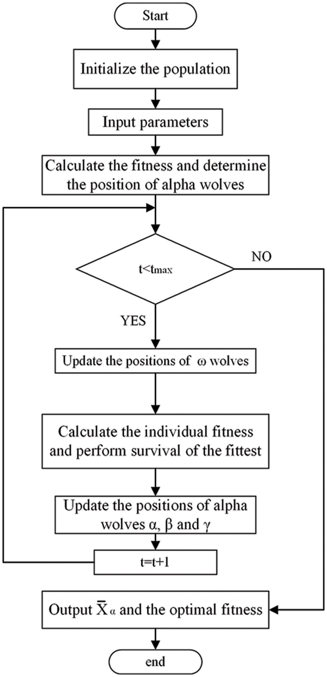
Figure 2: Algorithm flowchart

To evaluate the optimization ability and anti-premature convergence ability of the improved CS-GWO hybrid optimization algorithm and two basic optimization algorithms, the Sphere unimodal and the Rastrigin multimodal test functions are selected in this paper, respectively. The function expressions can be expressed as Eqs. (24) and (25).

f1(x)=∑i=1nxi2, (24)

f2(x)=∑i=1n[xi2−10cos(2πxi)+10]. (25)

The population size is uniformly set to 30 to ensure the fairness of the algorithm test. The algorithm is iterated 100 times and 1000 times in one-dimensional and multi-dimensional cases, respectively, with the probability of Pa=0.5 . Optimization intervals of the Sphere test function and the Rastrigin test function are [−100, 100] and [−10, 10], respectively, and the corresponding optimization steps a are 10 and 1, respectively. The test results are shown in Table 1.

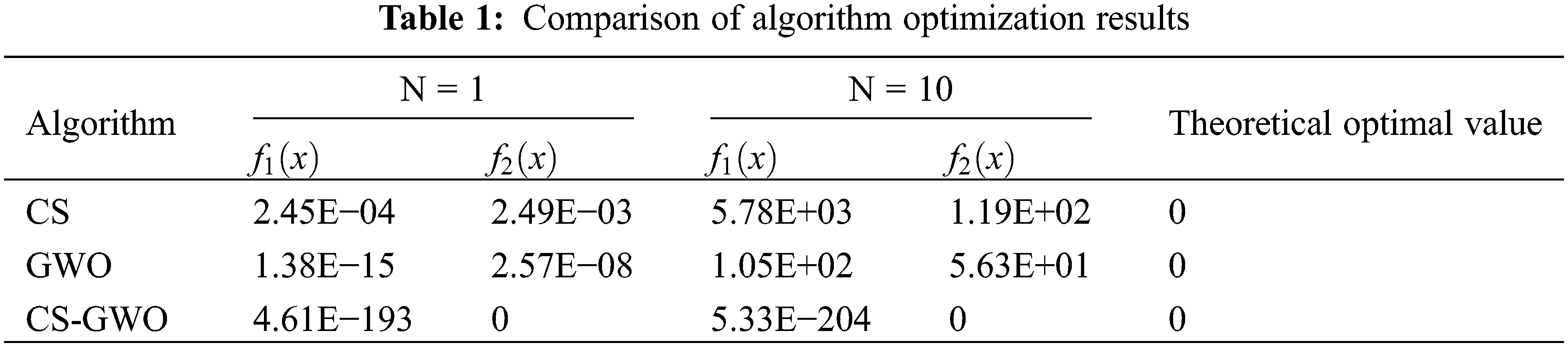
Since all test algorithms have random factors, the optimal values obtained in Table 1 are all taken as average values of the ten test results to reduce the error caused by randomness. Under the same test conditions, the improved optimization algorithm proposed in this paper can always obtain better results than the other two basic optimization algorithms. To further analyze the algorithm convergence, three algorithm convergence diagrams for the Rastrigin test function under the 10-dimensional condition are given as Fig. 3.

Figure 3: 10-dimensional Rastrigin test function algorithm convergence

As shown in Fig. 3, the basic CS algorithm can jump out of the local convergence in the middle and late stages of iterations. However, its convergence rate is too low. Although the basic GWO algorithm has a higher convergence rate in the early iteration stage, it falls into premature convergence after 100 iterations. Compared with the GWO and CS algorithms, the improved CS-GWO hybrid optimization algorithm proposed in this paper achieves a better convergence rate and can jump out of local convergence.

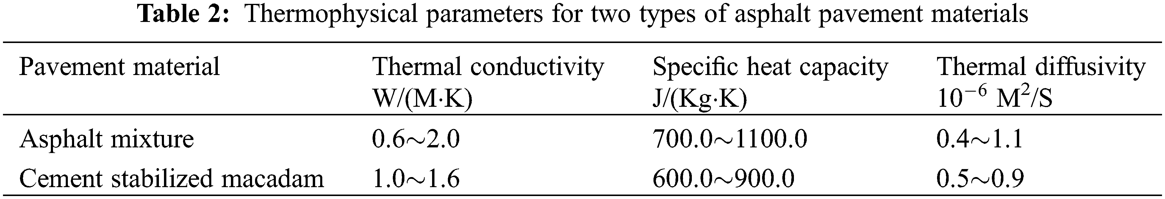
In the previous studies on the temperature field of asphalt pavement, the thermal performance parameters of pavement material were regarded as constants. Although this simplifies the calculation, it also affects the calculation accuracy. Since the test method for measurement is not simple and economical enough in practical application, an improved swarm intelligence optimization algorithm is selected in this paper to invert and analyze the variation laws on the thermophysical parameters of asphalt pavement materials with temperature, thereby obtaining more accurate numerical calculation results. The following maximum value range is taken for the thermal parameters of asphalt pavement materials to determine the inversion interval [30–32].

Compared with the base material, thermophysical parameters for asphalt mixture have a larger variation range, and their thermal conductivity is greatly affected by temperature. The research in [31] indicated that the thermal conductivity of asphalt mixture and cement-stabilized macadam could be fitted to a first-order linear function that varies with temperature in the actual temperature range of the asphalt pavement structure. Thus, a relatively high degree of fitting can be obtained. The research from [32] showed that the temperature of the asphalt mixture was also linearly related to thermal diffusivity. Therefore, considering the low-temperature sensitivity of specific heat capacity and density of asphalt pavement materials, the first-order linear function form for the change of thermal diffusivity of asphalt mixture and cement-stabilized macadam material with temperature is inverted in this paper. The differential equation for the inverse heat conduction problem of a one-dimensional structural layer of asphalt pavement can be expressed as:

α(T)∂2T(z,t)∂z2=∂T(z,t)∂t Hi−1<z<Hi,t>0, (26)

where α(T) denotes the functional form of the thermal diffusivity to be inverted. The structural parameters, boundary conditions, and initial temperature distribution of the model are fitted by high-order polynomials using the measured values for the experimental pavement structure layer. The inverted optimization objective function is determined as follows:

S=1MN∑i=1M∑j=1N(Tij∗−Tij|α(T)=AT+B)2, (27)

where M denotes the measured number of nodes in the temperature field of the asphalt pavement structure layer, for which the value is taken as five in this paper. Parameter N denotes the number of time nodes for temperature acquisition within 24 h, the value for which is taken as 144. Parameters T∗ and T denote the measured temperature and the numerically calculated temperature, respectively. Parameters A and B denote the parameters to be inverted, for which the inversion interval is determined by the value range of thermal diffusivity in Table 2 and the temperature variation range of the actual asphalt pavement structure. With the referent measured data, the daily variation interval for the temperature field of the high-temperature asphalt pavement is taken as range of 20 to 80 in this paper.

The inversion flow chart for the thermal diffusivity of asphalt pavement materials based on the improved CS-GWO hybrid swarm intelligence optimization algorithm in this paper is finally obtained as Fig. 4.

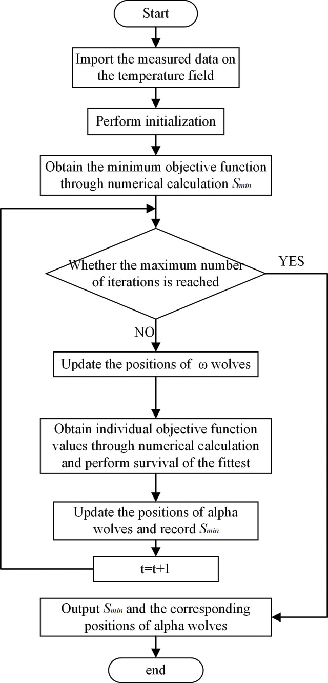
Figure 4: Flowchart for thermal diffusivity inversion of asphalt pavement materials

3  Results and Discussion

In this paper, the temperature at different depths of the test asphalt pavement and the external meteorological data are collected for research [33]. The monitoring experiment was carried out in September 2020 under the high temperature and no rain weather, and the data collection was carried out continuously for 24 h on a daily basis. Select the data with temperature greater than 55° from the observation points as the measured data for predictive analysis.

In combination with the monitored asphalt pavement structure parameters and temperature field data, the algorithm optimization probability Pa calculated through inversion in this paper is taken as 0.5. The optimization step sizes are taken as 0.4 × 10−7 and 0.2 × 10−7, in the range of asphalt pavement surface layer and base layer, respectively. The number of populations in the algorithm is set to 15. In the numerical calculation, the space step and time step are taken as 0.0025 m and 600 s, respectively. The actual monitoring data on the temperature field of asphalt pavement under the weather with high temperature and no rain is employed. The numerical inversion based on the improved CS-GWO hybrid swarm intelligence optimization algorithm is conducted on the thermal diffusivity of the base material and surface material of experimental asphalt pavement, respectively. Numerical inversion results of thermal diffusivity of pavement materials and the convergence diagram of the objective function on three typical high-temperature days are shown in Table 3.

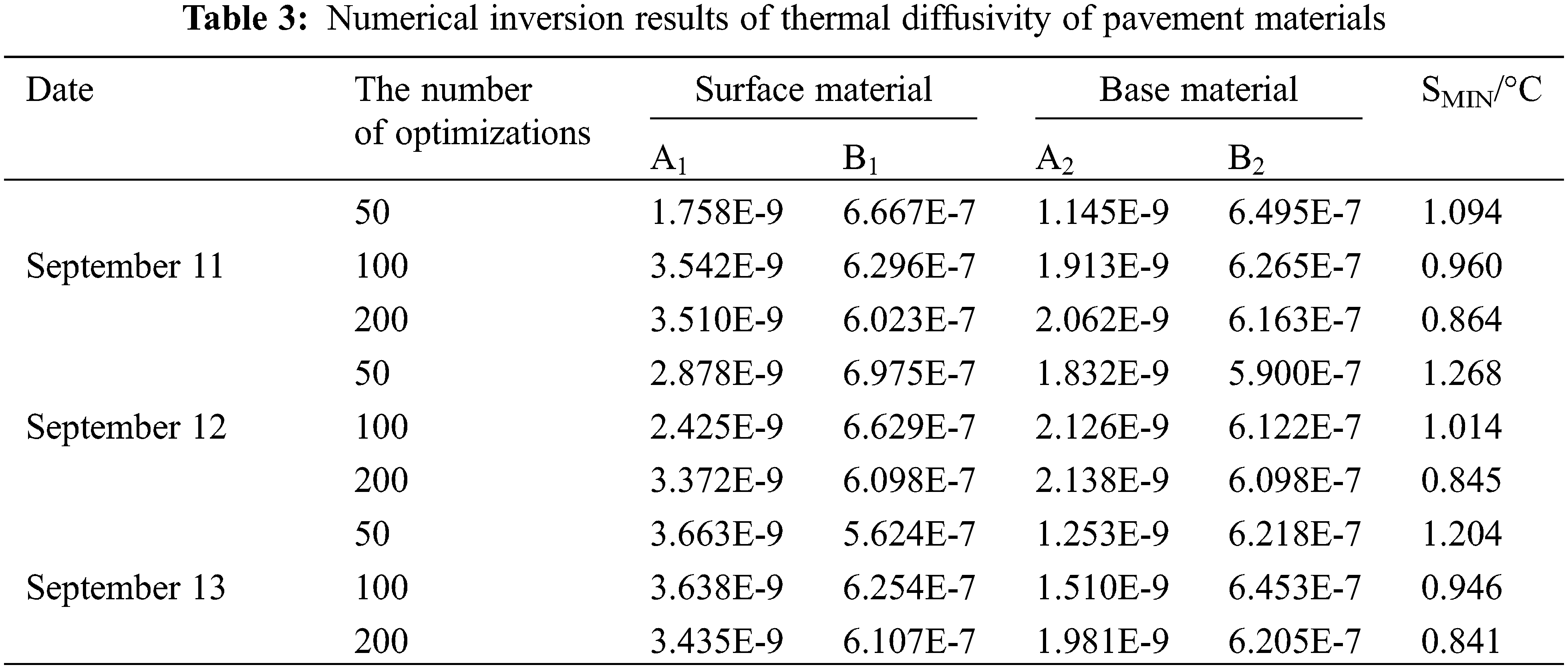
According to Table 3, the inversion results of the same asphalt pavement based on the measured data of the temperature field on different dates are roughly the same, which indicates the accuracy of the inversion results. The linear relationship of thermal diffusivity of the surface material and the base material of experimental asphalt pavement with temperature can be determined according to the average values of coefficients A and B obtained by inversion, as shown in Eqs. (28) and (29).

α1(T)=3.439×10−9T+6.076×10−7, (28)

α2(T)=2.060×10−9T+6.155×10−7. (29)

The measured data of pavement temperature field are used as the single value condition of the calculation model to evaluate the accuracy of the numerical inversion and calculation method applied in predicting the actual temperature field of asphalt pavement. After determining the single value condition, the nonlinear numerical calculation is performed based on the inversion results for the thermal diffusivity of pavement material. The calculation results for the temperature field of asphalt pavement at two different depth positions, the accurate solution calculation results for the temperature field of double-layer pavement, and the measured values are selected for comparison, as shown in Figs. 5 and 6, Table 4.

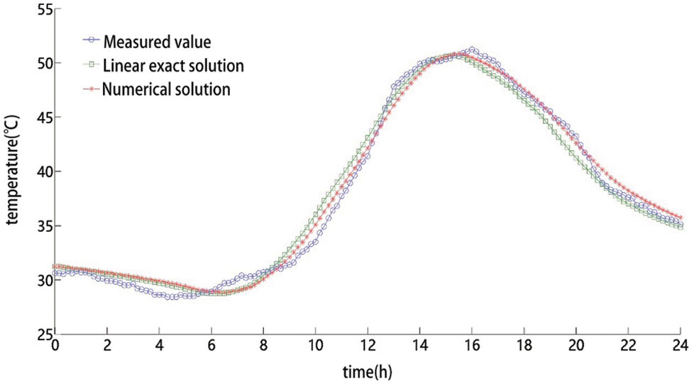
Figure 5: Comparison of predicted temperature results at 0.05 m depth on September 12

Figure 6: Comparison of predicted temperature results at 0.15 depth m on September 12

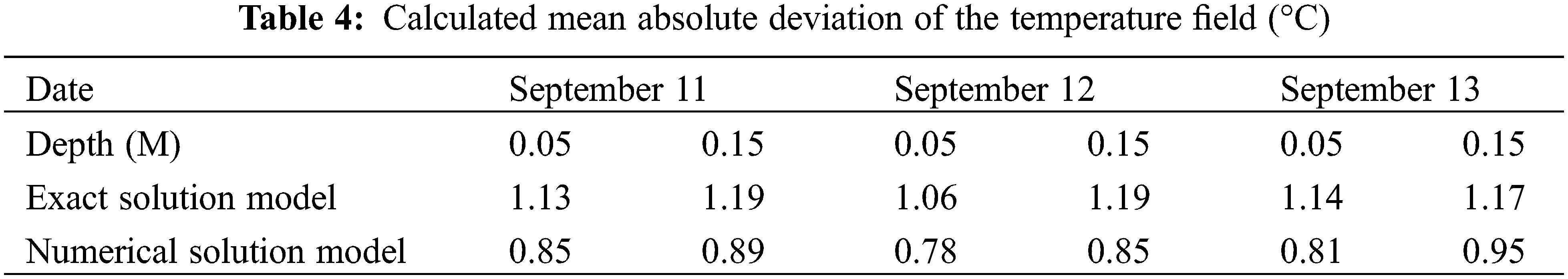
Due to errors in the upper boundary conditions of the calculation model, the numerical calculation results for most time points in a single day in Figs. 5 and 6 are closer to the measured values than the calculation results of the exact linear solution. For the three typical high-temperature days in Table 4, the predicted mean absolute deviation of the numerical solution model is 0.297°C lower than that of the exact solution model at a depth of 0.05 m. At a depth of 0.15 m, the predicted mean absolute deviation of the numerical solution model is 0.287°C lower than that of the exact solution model. The numerical prediction of the temperature field based on the finite difference method has higher accuracy than the linear exact solution prediction when considering the change in the thermal diffusivity of pavement material.

It can be considered that the numerical prediction of temperature field based on finite difference method is more accurate than the linear exact solution when considering the change of thermal diffusion coefficient of pavement materials. Compared with the previous calculation methods based on empirical constants, the numerical prediction model of nonlinear asphalt pavement temperature field elaborated based on numerical inversion and finite difference method has better effect.

4  Conclusions

Contrary to the previous calculation methods for temperature fields that only consider thermophysical parameters of pavement materials as constants empirically, the improved CS-GWO hybrid swarm intelligence optimization algorithm was proposed in this paper. The algorithm is used for numeric inversion of thermal diffusivity of pavement materials. Then, the nonlinear numerical prediction of the asphalt temperature field is performed based on the finite difference method. The following conclusions are drawn:

(1)   In this study, the implicit difference scheme of pavement temperature field is derived by Taylor series expansion method. According to the structural parameters of the experimental pavement, the position of the temperature sensor and the stability conditions of the difference scheme, the space step and the time step of the temperature field numerical calculation are determined, the temperature field is discretized, and the nonlinear numerical calculation method of the pavement temperature field is determined.

(2)   The Levy flight mechanism and the wolf pack hunting mechanism were employed to optimize the algorithm structure and the optimal position updating formula. Then, an improved CS-GWO hybrid swarm intelligence optimization algorithm was proposed. An optimization test was performed on the improved algorithm via the Sphere unimodal test function and the Rastrigin multimodal test function with different dimensions. The test results show that the improved algorithm proposed in this paper is better than the CS algorithm and the GWO algorithm in terms of convergence rate and optimization ability.

(3)   On three typical high-temperature days, at a depth of 0.05 m, the predicted mean absolute deviation of the numerical solution model is 0.297°C lower than that of the exact solution model. At a depth of 0.15 m, the predicted mean absolute deviation of the numerical solution model is 0.287°C lower than that of the exact solution model.

This study can be used to accurately predict the temperature field of high-temperature asphalt pavement. Consequently, the relationship between the external environment, the asphalt pavement quality, and safety risk level in high-temperature seasons can be obtained.

Funding Statement: The authors received no specific funding for this study.

Conflicts of Interest: The authors declare that they have no conflicts of interest to report regarding the present study.

References

    1. Zhu, H., Cai, H., Wen, X., Cao, R. (2019). Evaluation on the high temperature performance of intermediate and bottom layers of asphalt pavement in service. Transportation Research Congress 2017: Sustainable, Smart, and Resilient Transportation, pp. 312–322, Reston, VA: American Society of Civil Engineers. [Google Scholar]

    2. Sun, J., Wei, B., Zhang, Y., Yang, J. (2020). Experimental study on high-temperature stability of rubber powder-modified asphalt mixture. Journal of Physics: Conference Series, 1605(1), 012160. DOI 10.1088/1742-6596/1605/1/012160. [Google Scholar] [CrossRef]

    3. Robertson, W. D. (1997). Determining the winter design temperature for asphalt pavements (with discussion and closure). Journal of the Association of Asphalt Paving Technologists, 66, 312–343. [Google Scholar]

    4. Nam, K. (2005). Effects of thermo-volumetric properties of modified asphalt mixtures on low-temperature cracking (Ph.D. Thesis). The University of Wisconsin-Madison, USA. [Google Scholar]

    5. Velasquez, R., Tabatabaee, H., Bahia, H. (2011). Low temperature cracking characterization of asphalt binders by means of the single-edge notch bending (SENB) test. Journal of the Association of Asphalt Paving Technologists, 80, 583–613. [Google Scholar]

    6. Olubukola, O., Tokede, A. W., Rose, M., Marzia, T. (2020). Life cycle assessment of asphalt variants in infrastructures: The case of lignin in Australian road pavements. Structures, 25(7), 190–199. DOI 10.1016/j.istruc.2020.02.026. [Google Scholar] [CrossRef]

    7. Seyed, R. O., Michiel, G., Myrthe, V. H., Navid, H. (2022). Assessing the potential of application of titanium dioxide for photocatalytic degradation of deposited soot on asphalt pavement surfaces. Construction and Building Materials, 350, 128859. [Google Scholar]

    8. Hamid, J., Mohammad, M. K., Hamed, N., Fereidoon, M. N. (2020). Sustainable asphalt concrete containing high reclaimed asphalt pavements and recycling agents: Performance assessment, cost analysis, and environmental impact. Journal of Cleaner Production, 244(1), 118837. DOI 10.1016/j.jclepro.2019.118837. [Google Scholar] [CrossRef]

    9. Aletba, S., Hassan, N. A., Jaya, R. P., Aminudin, E., Mahmud, M. et al. (2021). Thermal performance of cooling strategies for asphalt pavement: A state-of-the-art review. Journal of Traffic and Transportation Engineering (English Edition), 8(3), 356–373. [Google Scholar]

  10. Lu, R., Jiang, W., Xiao, J., Xing, C., Chong, R. et al. (2022). Temperature characteristics of permeable asphalt pavement: Field research. Construction and Building Materials, 332(12), 127379. DOI 10.1016/j.conbuildmat.2022.127379. [Google Scholar] [CrossRef]

  11. Zhang, X., Chen, E., Li, N., Wang, L., Si, C. (2022). Micromechanical analysis of the rutting evolution of asphalt pavement under temperature-stress coupling based on the discrete element method. Construction and Building Materials, 325(1), 126800. DOI 10.1016/j.conbuildmat.2022.126800. [Google Scholar] [CrossRef]

  12. Zhao, K., Yan, G., Li, J., Wang, L. (2021). Study on fracture characteristics of asphalt pavement with longitudinal and transverse cracks under the influence of real temperature field. IOP Conference Series: Earth and Environmental Science, 719(3), 032072. DOI 10.1088/1755-1315/719/3/032072. [Google Scholar] [CrossRef]

  13. Christison, J. T., Anderson, K. O. (1972). The response of asphalt pavements to low temperature climatic environments. International Conference on the Structural Design of Asphalt Pavements, London. [Google Scholar]

  14. Mohammad, Z. A., Mohammad, R. P. (2018). Prediction of asphalt pavement temperature profile with finite control volume method. Transportation Research Record, 2456(1), 96–106. [Google Scholar]

  15. Chandrappa, A. K., Biligiri, K. P. (2016). Development of pavement-surface temperature predictive models: Parametric approach. Journal of Materials in Civil Engineering, 28(3), 04015143.1–04015143.12. DOI 10.1061/(ASCE)MT.1943-5533.0001415. [Google Scholar] [CrossRef]

  16. Qin, Y. (2016). Pavement surface maximum temperature increases linearly with solar absorption and reciprocal thermal inertial. International Journal of Heat & Mass Transfer, 97(8), 391–399. DOI 10.1016/j.ijheatmasstransfer.2016.02.032. [Google Scholar] [CrossRef]

  17. Wang, D. (2016). Prediction of time-dependent temperature distribution within the pavement surface layer during fwd testing. Journal of Transportation Engineering, 142(7), 6016001–6016002. DOI 10.1061/(ASCE)TE.1943-5436.0000854. [Google Scholar] [CrossRef]

  18. Xu, B., Dan, H. C., Li, L. (2017). Temperature prediction model of asphalt pavement in cold regions based on an improved BP neural network. Applied Thermal Engineering, 120(4), 568–580. DOI 10.1016/j.applthermaleng.2017.04.024. [Google Scholar] [CrossRef]

  19. Liu, S., Han, S., Chen, H., Li, Z. (2019). Research on pavement temperature prediction based on neural network. IOP Conference Series: Earth and Environmental Science, 300(3), 032067. DOI 10.1088/1755-1315/300/3/032067. [Google Scholar] [CrossRef]

  20. Ozisik, M. N. (1980). Heat conduction. Wiley, Wiley-Interscience Publishing. [Google Scholar]

  21. Ozisik, M. N. (1985). Heat transfer. McGraw-Hill, Joule Library 53602/OZI. [Google Scholar]

  22. Bernatz, R. A. (2010). The finite difference method. In: Bernatz, R. A. (Ed.Fourier series and numerical methods for partial differential equations. DOI 10.1002/9780470651384.ch9. [Google Scholar] [CrossRef]

  23. Yang, X. S., Deb, S. (2009). Cuckoo search via Lévy flights 2009. World Congress on Nature & Biologically Inspired Computing (NaBIC), Coimbatore, IEEE. [Google Scholar]

  24. Yang, X. S., Deb, S. (2010). Engineering optimisation by cuckoo search. International Journal of Mathematical Modelling & Numerical Optimisation, 1(4), 330–343. DOI 10.1504/IJMMNO.2010.035430. [Google Scholar] [CrossRef]

  25. Chi, X., Yu, B., Jiang, X. (2019). Parameter estimation for the time fractional heat conduction model based on experimental heat flux data. Applied Mathematics Letters, 102, 106094. [Google Scholar]

  26. Mirjalili, S., Mirjalili, S. M., Lewis, A. D. (2014). Grey wolf optimizer. Advances in Engineering Software, 69, 46–61. DOI 10.1016/j.advengsoft.2013.12.007. [Google Scholar] [CrossRef]

  27. Saremi, S., Mirjalili, S. Z., Mirjalili, S. M. (2015). Evolutionary population dynamics and grey wolf optimizer. Neural Computing & Applications, 26(5), 1257–1263. DOI 10.1007/s00521-014-1806-7. [Google Scholar] [CrossRef]

  28. Song, X., Tang, L., Zhao, S., Zhang, X., Li, L. et al. (2015). Grey wolf optimizer for parameter estimation in surface waves. Soil Dynamics and Earthquake Engineering, 75(3), 147–157. DOI 10.1016/j.soildyn.2015.04.004. [Google Scholar] [CrossRef]

  29. Gupta, S., Deep, K. (2018). A novel random walk grey wolf optimizer. Swarm and Evolutionary Computation, 44, 101–112. [Google Scholar]

  30. Jia, L., Sun, L., Yu, Y. (2007). Asphalt pavement statistical temperature prediction models developed from measured data in China. Seventh International Conference of Chinese Transportation Professionals Congress (ICCTP), pp. 723–732. Shanghai, Tongji University. [Google Scholar]

  31. Yan, X., Chen, L., You, Q., Fu, Q. (2019). Experimental analysis of thermal conductivity of semi-rigid base asphalt pavement. Road Materials and Pavement Design, 20(5–6), 1215–1227. DOI 10.1080/14680629.2018.1431147. [Google Scholar] [CrossRef]

  32. Chadbourn, B. A., Newcomb, D., Voller, V., Desombre, R. A., Luoma, J. A. et al. (1998). Asphalt paving tool for adverse conditions. University of Minnesota Digital Conservancy. https://hdl.handle.net/11299/1035. [Google Scholar]

  33. Jiang, Z. H., Wang, Q., Zhou, L. B. (2022). Analysis of measured and theoretically predicted temperature field in high-temperature asphalt pavement during daily cycle. Forest Chemicals Review, 1–17. [Google Scholar]