Simulation of Vertical Solar Power Plants with Different Turbine Blades

1  Introduce

In recent years, with the economy’s rapid development all over the world, the energy consumption rate has continued to rise, and the air pollution becomes serious. Although the total resources are considered rich on the earth, the per capita recoverable fossil energy reserves show a downward trend [1].

At present, mainly fossil energy consumption is coal. There are problems such as low source utilization efficiency and serious environmental pollution. Therefore, it is very urgent to speed up the change in energy consumption structure and actively look for alternative new energy [2].

As a new energy source, solar energy has attracted widespread attention due to its abundant reserves, cleanliness, and environmental protection advantages. As a new type of solar power generation equipment, Professor Schlaicha first proposed vertical solar power stations in 1978. Improving energy conversion efficiency is the main research direction for solar power plants, and the blade airfoil of a turbine blade impacts the power plant efficiency. In the 1980s and 1990s, the world’s first solar thermal power station was built, which is still in operation [3]. Several types of solar chimney models were established, and a lot of theoretical and experimental research are carried out [4].

Since the 20th century, Zhou et al. [5–8], and others have conducted experimental research on the overall system of the solar thermal airflow power station. Wang et al. [9] analyzed the internal blades and got the aerodynamic performance comparison results of the vertical fan airfoil of NACA0018 and NACA4418. And Wang also proposed the performance advantages and disadvantages of the two airfoils under different tip speed ratios. Jia et al. [10] studied the single blade pressure, speed, and lift-drag coefficient of four profiles under different wind speeds and concluded that NACA0018 has the best aerodynamic performance. Wu et al. [11,12] conducted a simulation study on the influence of different turbulence models on the calculation results of airfoils. The results showed that the drag coefficient of the SST K − ω turbulence model was closer to the experimental value. In addition, Wu et al. [11,12] studied the influence of the angle of attack and relative thickness on the aerodynamic performance, conducted a numerical simulation of the twist angle and aerodynamic characteristics of the NACA4415 airfoil, and proposed the twist angle at the maximum lift-drag ratio. Xu et al. [13] used a genetic algorithm and Wilson theory to calculate blade shape parameters with better aerodynamic performance. Yu et al. [14] used biosimulation technology to optimize the shape of the NACA0015 airfoil to increase the lift-drag coefficient and improve the airfoil surface. Zhao et al. [15,16] explored different blades, and obtained blade parameters with practical significance.

Gang et al. [17] used the secondary curve to fit the turbine runner blade by parameter, changed the proportion coefficient of the blade partial position, and controlled the shape of the blade. The research results showed that the efficiency after changing the shape was increased by 2.5%. Fan et al. [18] conducted orthogonal experiments on the blade airfoil and blade number of the axial flow impeller. The results showed that the blade airfoil had the greatest influence on the axial flow impeller’s full-pressure performance and efficiency. Li et al. [19] chose two existing airfoils to design the new airfoil and simulated numerically. The results showed that the power of the three-blade turbine composed of the new wing increased by 16% and 30% higher than the initial two blades.

There are also studies on turbine blades in aerospace. Mei et al. [20] carried out an aerodynamic analysis on aero-engine turbine blades. Using numerical simulation, they got the total stress, strain, and deformation nephogram of blades under typical working conditions. In the article, the author analyzed the stress condition of the blades under specific working conditions and provided data support for blade structure design and life prediction of specific working conditions. Wei et al. [21] used finite element analysis technology to analyze the deformation, stress, and other parameters of the two groups of blades under centrifugal load. By analyzing the data, they got the large differences in the blades’ performance to predict the blades’ future development trend. However, despite the large differences in the application conditions of the turbine of aerospace and solar power plants, the volume of the turbine is also different. However, due to the great differences in the application conditions of turbines of aerospace and solar power plants, the volume of turbines is different. It has not been determined whether the influence law of space turbine blade number, chord length, and torsion angle on turbine power can be directly applied to the turbines of solar power plants. Therefore, it is necessary to study the relevant parameters of turbines suitable for solar power plants.

The power generation principle of a vertical solar power station is shown in Fig. 1 [22]. The system is simple in structure and easy to maintain. It mainly comprises a chimney, heat collecting shed, and turbine generator. After the system is installed, the power generation mode is simple. The turbine is the only complex component in this system, and it is also the component that has the greatest impact on the system’s power. The blades in the turbine have a great impact on the efficiency of the turbine. The research on the blade airfoil is conducive to the further utilization of solar energy resources. Most of the research is focused on the influence of the blade tip speed ratio, angle of attack, and other parameters on performance. There is less research on the relationship between blade shape and aerodynamic performance. The turbine’s performance can be optimized by studying the blade shape parameters such as chord length and torsion angle, which greatly impact the turbine’s aerodynamic performance. At the same time, it provides some references for other researchers. To further study the influence of turbine blade airfoil on the overall efficiency, this paper plans to design the blade based on Wilson’s theory and carry out a numerical simulation of the three-dimensional model. The research results have certain guiding significance for selecting airfoils and improving turbine performance in the future.

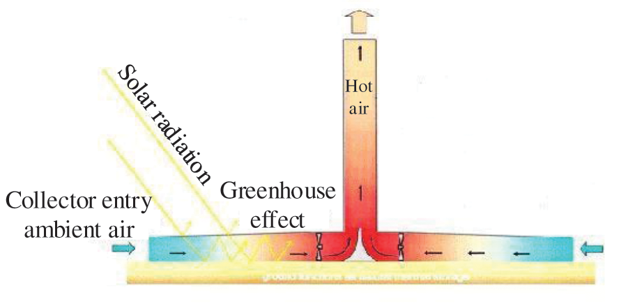
Figure 1: Solar power station schematic

2  The Mathematical Model for Blade Design

The blade design based on the assumptions of the Bates theory [23] and the momentum theory [24] introduces an axial induction factor a and a circumferential induction factor b. a and b represent the influence of the impeller on the air axial velocity and the correction coefficient of the impeller on the radial disturbance of the wind speed, respectively. Bates’ theory refers to the reduction of the turbine to an ideal state. The turbine hub is ignored in the calculation process, and momentum theory ignores momentum changes other than the axial direction. Blade-element theory’s simplification of the model ignores the loss at the tip and root. In order to reduce the error, the tip and heel loss coefficients F = Ftip = Fhub are introduced for correction [25].

Using Wilson’s theory to design and draw the simulated blade. Under the careful consideration of losses and working conditions, by summarizing and improving the above methods, a new design model is proposed [26]:

dCpdλ=−8λ02b(1−a)Fλ3 (1)

b(1+b)λ2=a(1−aF) (2)

where, Cp is the wind energy utilization coefficient, Cp = ΩM⋅(0.5 ρV 3S); λ is the tip speed ratio of a section, λ = ωr/V1; S is the swept area of the rotor, m2; Ω is the rotational speed of the rotor, rad/s; M is the torque of the rotor; F is the resistance correction coefficient.

3  Blade Design Geometric Model

3.1 Selection of Blade Parameters

At present, the commonly used turbine blades are mainly NACA series and Ames series airfoils. Considering the strength of the blade and the blade root then, the simulation process selects NACA63212 and AMES63212 airfoils for blade design. There is a certain relationship between the number of blades and the turbine’s power. When running at a low wind speed, a larger number of blades can get a larger wind energy utilization factor and better starting characteristics. With the increased number of blades, the airflow can produce greater impulse when passing through the blades so the turbine can get greater torque and output power. However, when the number of blades is too much, the flow resistance increases, and the flow through the turbine decreases. And the hub will limit the amount of impeller installation. Considering the actual situation, the number of blades selected in this paper is 7 and 8; the wind speed is 3–6 m/s; the initial tip speed ratio λ0 = 3.

3.2 Parameter Calculation

The calculation of blade parameters is mainly axial a and circumferential induction factors b [27]. The initial value at the time of calculation is:

a=λ022000+0.027λ0−0.038 (3)

b=10λ0e12rR (4)

The Matlab program is written with formula (3) as the objective function and formula (4) as the constraint condition for iterative calculation. The chord length and torsion angle are calculated using the iteratively got a and b values.

The comparison results of the two airfoils after linear correction of the blade parameters are shown in Fig. 2.

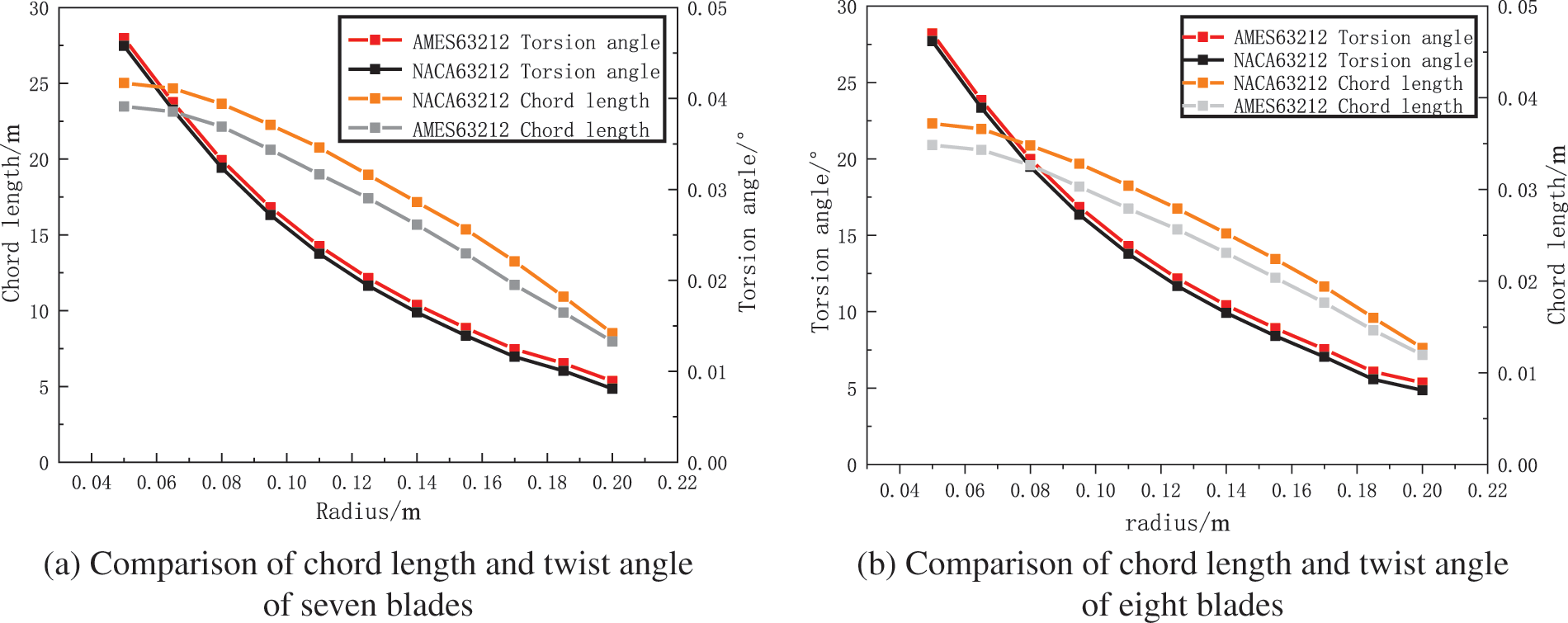
Figure 2: Comparison of two airfoil chord lengths and twist angles

In Fig. 2, the various laws of the chord length and twist angle of the two airfoils are the same under different numbers of blades. The variation law of chord length and twist angle with blade element radius can be obtained by fitting the data, as shown in Eqs. (5) and (6).

L=−0.6641r2−0.0219r+0.045R2=0.9991 (5)

I=47.777e−10.89rR2=0.9996 (6)

where, L is the chord length, m; I is the torsional angle, °; r is the blade radius, m; R2 is the fitting accuracy, and the closer R2 is to 1, the higher the accuracy is.

Under the same number of blades, the NACA63212 airfoil is flatter and has less torsional change. The result is the NACA63212 airfoil has a higher chord than the other airfoil and a smaller twist angle.

The quality of the blades directly affects the efficiency of the turbine, and the lift-drag ratio is an important indicator for evaluating the turbine’s performance. Generally, a higher wind resistance ratio is required in the design. Fig. 3 shows the lift-drag ratio of the two-airfoil single blade.

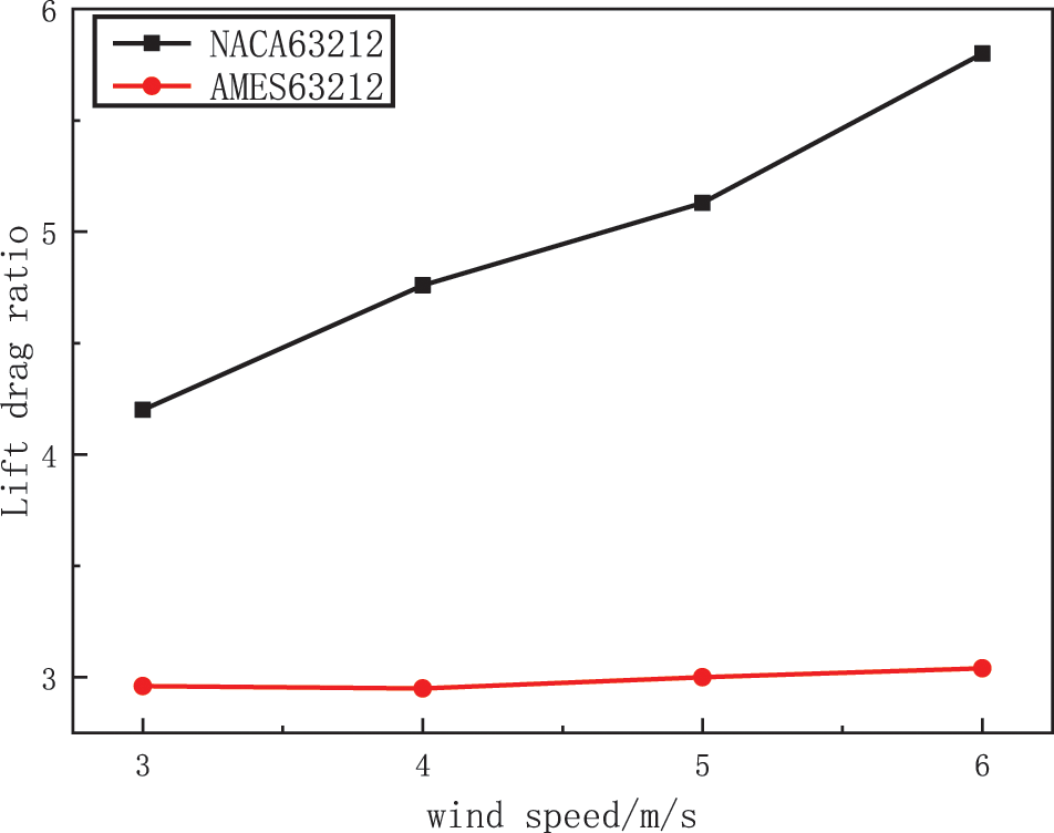
Figure 3: Airfoil lift drag ratio

As demonstrated in Fig. 3, under the same conditions, the lift drag of the NACA63212 airfoil is higher than that of the AMES63212 airfoil. For the NACA63212 airfoil, lift increases faster than drag at low wind speeds, so the overall lift-to-drag ratio increases with wind speed. The lift-drag ratio is primarily unaffected by changes in wind speed in the AMES63212 airfoil, which has a modest difference between lift and drag increments. The lift-drag ratio is the result of the interaction of multiple blades. The interaction between several blades will significantly alter the lift and resistance, even if it is not immediately apparent how the chord length and torsion angle of the two blades compare.

3.3 3 D Geometric Models of the Blade

Convert the (x, y) coordinates in the airfoil library to 3D coordinates. Import the three-dimensional coordinates in SolidWorks to draw the blade. The blade element of the two airfoils, as shown in Fig. 4.

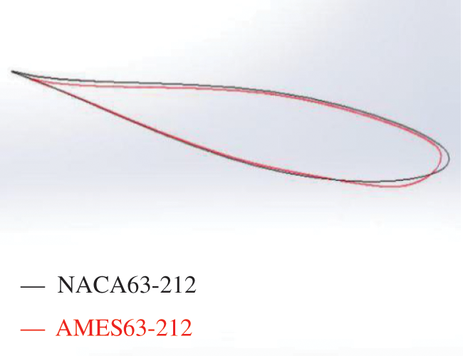
Figure 4: Comparison of blade elements of two types of the airfoil

In Fig. 4, there is a difference in the blade element between the two airfoils at a diameter of 0.1 m, and the blade element shape of the NACA63212 blade is slightly larger than the root.

4  Numerical Simulation and Airfoil Performance Analysis

4.1 Numerical Computation Model

The law of conservation of mass in fluid flow [28] is:

∂ρ∂t+∂(ρu)∂x+∂(ρv)∂y+∂(ρw)∂z=0 (7)

Because the density of an incompressible fluid is constant, the continuity equation is:

∂u∂x+∂v∂y+∂w∂z=0 (8)

where, u, v and w represent the component of the velocity in the x, y, z direction, m/s.

The generalized source terms of the three momentum equations are defined as Su, Sv and Sw, which are substituted into the momentum equations and written in vector form:

∂(ρu)∂t+div(ρuU→)=div(η⋅gradu)+Su−∂p∂x (9)

∂(ρv)∂t+div(ρvU→)=dv(η⋅gradv)+Sv−∂p∂y (10)

∂(ρw)∂t+div(ρwU→)=div(η⋅gradw)+Sw−∂p∂z (11)

If the fluid is an incompressible fluid, the Su = Sv = Sw = 0. The upper equations can be simplified to:

∂u∂t+dv(uU→)=dv(ν⋅gradu)−1ρ∂p∂x (12)

∂v∂t+dv(vU→)=dv(ν⋅gradv)−1ρ∂p∂y (13)

∂w∂t+dv(wU→)=dv(ν⋅gradw)−1ρ∂p∂z (14)

where, U→ represents the velocity vector, m/s; v (v = μ/ρ) represents the dynamic viscosity of the fluid, m2/s; ρ represents the fluid density, kg/m3; p represents the pressure, Pa.

The SST K − ω turbulence model is developed from the standard K − ω turbulence model by Menter to achieve better accuracy and stability in the near-wall region. The SST K − ω turbulence model is obtained by combining the standard K − ε model with the K − ω turbulence model. Therefore, the SST K − ω turbulence model has more extensive applicability [29]:

∂∂t(ρk)+∂∂xi(ρku¯i)=∂∂xj(Γk∂k∂xj)+Fk−Yk (15)

∂∂t(ρω)+∂∂xi(ρωu¯j)=∂∂xi(Γω∂k∂xi)+Fω−Yω+Dω (16)

where, k is the turbulent kinetic energy; t is the time; ρ is the density, kg/m3; ui and uj are the average turbulent velocities; xi and xj are coordinate components; ω is the special dissipation of turbulence; Γk and Γω are the effective diffusion coefficient; Fk and Fω is turbulence generating item; Yk and Yω is the dissipation term of k and ω; Dω is the diffusion term; S is the shear force constant term; F2 is a mixed function

The turbulent dynamic viscosity coefficient of the SST K − ω turbulence model is:

μt=ρkωmax(SF2αω) (17)

where, α is the empirical constant term; S is the shear force constant term; F2 is a mixed function.

Using the above equations, the relevant data on the blade can be obtained. Then the models can be further established by the Design Modeler.

4.2 Grid Independence and Model Accuracy Verification

Import the saved file into the Design Modeler to build the model. The fluid region is separated into two parts, known as the inner field and outer field, to replicate the rotating flow of wind in specific locations and to make the simulation test more realistic. After establishing the entity, the Boolean operation is performed, and the division result shows in Fig. 5.

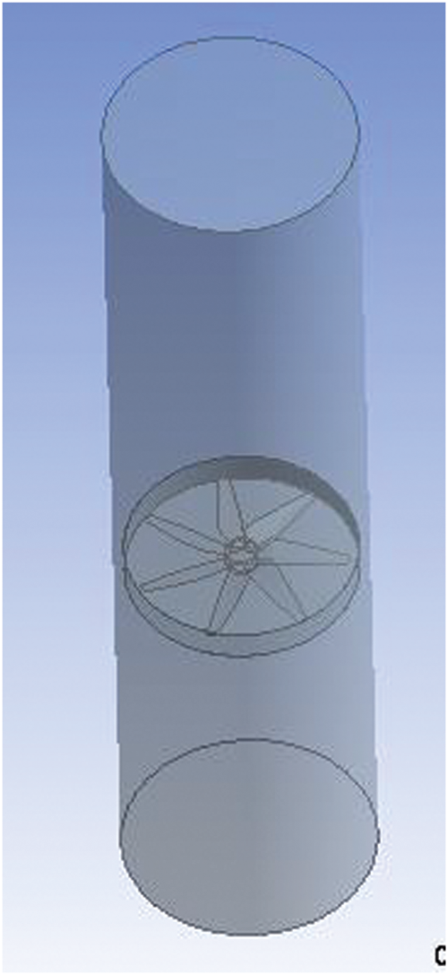
Figure 5: Simulated solid model

Bring the solid into GIMBIT for meshing. After the Boolean operation, it is necessary to merge the inner field’s upper and lower planes with the outer field’s corresponding planes, and then start the grid division. First, divide the impeller into line mesh and the impeller surface. The mesh shape is selected as Triangle. Following the completion of the volume mesh, it is needed to merge the inner field’s sides, and dividing the diffusion mesh is needed. Then, the independent verification was carried out on the eight-blade wind speed of 5 m/s. The verification results are shown in Fig. 6.

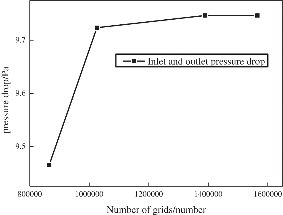
Figure 6: Grid-independent validation

It can be seen from Fig. 6 that when the number of mesh exceeds 1,389,214, the pressure drop at the inlet and outlet does not change. In order to save calculation time and ensure calculation accuracy, the number of mesh is set at about 1,400,000 during mesh division.

To ensure the correctness of the simulation model, it is necessary to choose the NACA63215 wing data to simulate with the above method, and get the power of 7 blades at different wind speeds. And compared with the experimental data obtained under the same blade parameters, the comparison results are shown in Fig. 7.

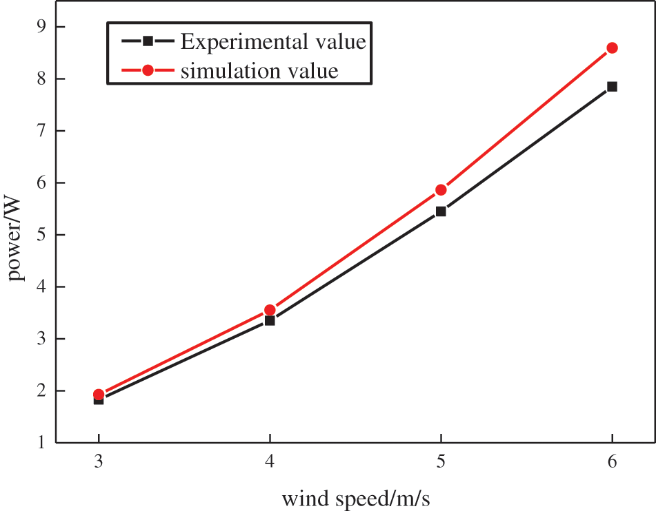
Figure 7: Model accuracy validation

To ensure the correctness of the model, the NACA63215 airfoil data is selected for simulation by the above method. The calculation results show that when the number of blades is seven and the wind speed is 4 m/s, the simulated torque is 0.0705 N/m, and the power is 5.3 W. Compared with the experimental data in reference [27], the error is 10%. Among them, the chord length of NACA63215 is the largest among the three airfoils, and the twist angle is the smallest.

4.3 Uniqueness Condition Settings

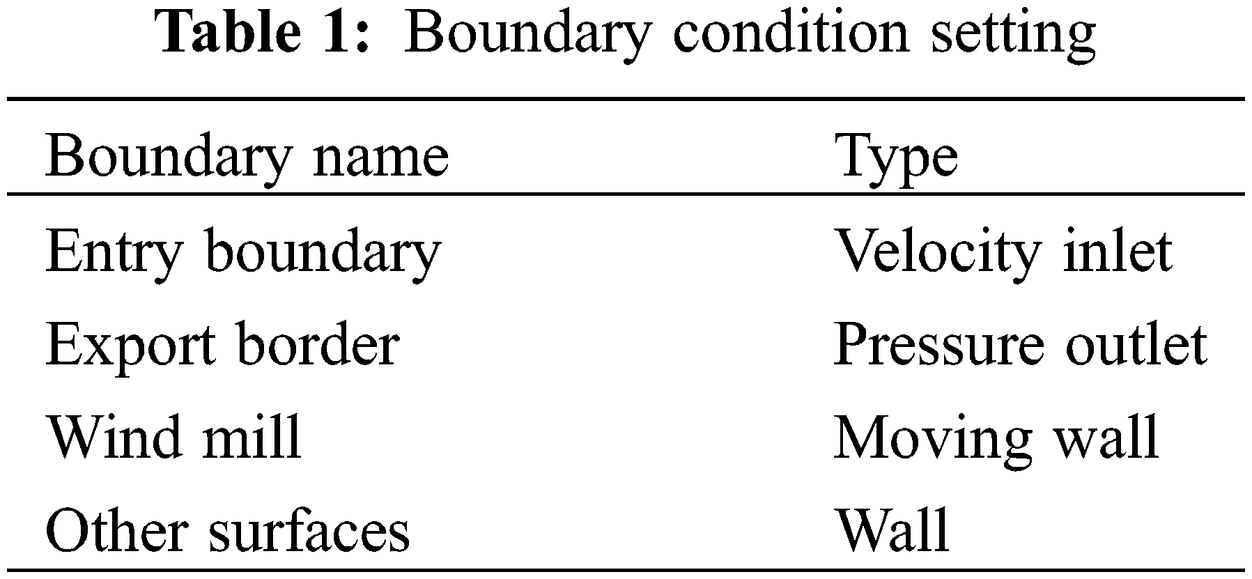
4.3.1 Boundary Condition Setting

The effect of gravity needs to be considered when setting conditions. In order to ensure the accuracy of the experiment, the residual value is set to 1 × 10−5. The boundary conditions are set as shown in Table 1.

4.3.2 Solver Settings

When setting the solver, the SIMPLEC algorithm is used to solve the pressure-velocity coupling. The pressure is discretized by the Presto scheme, which is more effective in dealing with the rotating flow with a large pressure gradient, and the second-order upwind scheme discretizes the others. The circumferential velocity of the blade tip is quite high despite the low incoming wind speed, creating complicated three-dimensional turbulence and SST K − ω. The turbulence model is widely used and has high accuracy and stability near the wall. References [11,12] have compared different turbulence models. Therefore, the turbulence model SST K − ω is selected for calculation. Other parameters remain at default values.

4.4 Simulation Results and Data Processing

In the Fluent simulation, the simulation test is carried out by changing the blade airfoil, the number, and setting different wind speeds. The simulation makes it possible to get the velocity and pressure contours of the two airfoils at different wind speeds. Take the interception from the middle of the blade, and get the velocity cloud map as shown in Fig. 8.

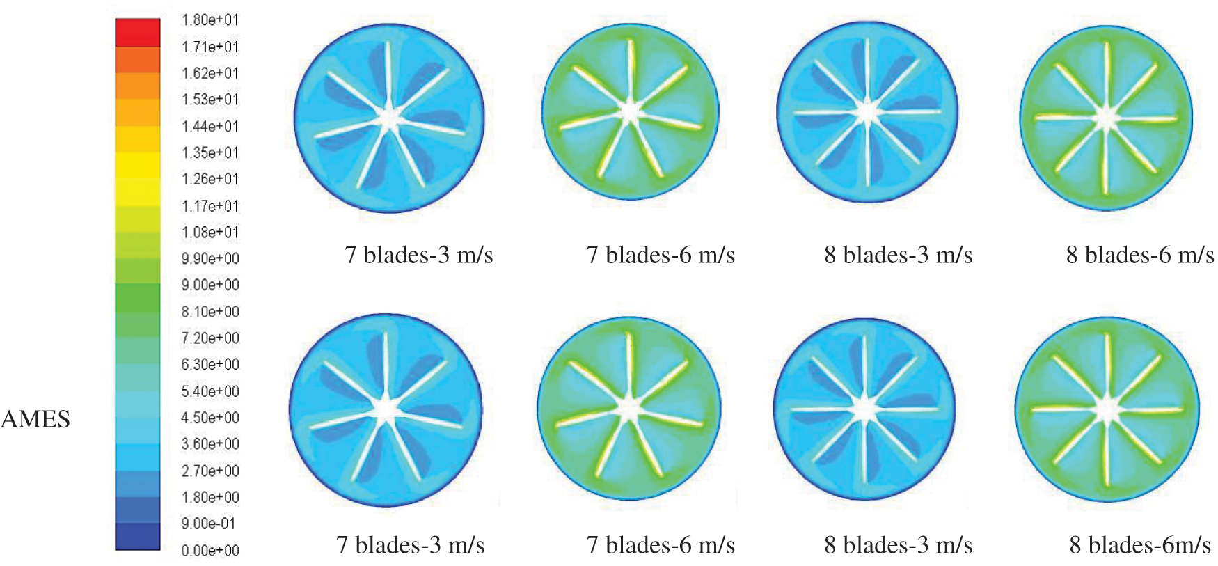
Figure 8: Velocity contour of the middle section of the blade

Both types of blades produce larger low-speed zones at lower wind speeds, as seen in Fig. 8. The low-speed area on the leeward side of the blades of the AMES63212 airfoil is significantly larger than that of the NACA63212, which harms the airfoil’s blades’ power of the AMES63212. The low-speed area distribution of the blades of the NACA63212 airfoil is more uniform than that of the AMES63212 airfoil when there are eight blades and a wind speed of 3 m/s. The difference between the velocity cloud diagrams of the two blades is small due to the large air velocity around the blade at 6 m/s wind speed.

The longitudinal pressure cloud map of NACA63212 with seven and eight blades is intercepted when the wind speed is 3 m/s, as shown in Fig. 9. When there are seven blades, the blades will significantly reduce the pressure of the passing airflow, and the low-pressure area is approximately symmetrically distributed. Because the kinetic energy brought by the thermal flow has a conversion of shaft work. When there are eight blades, there is a conversion of shaft work, but the eight blades are symmetrically distributed, so the total pressure drop after the airflow passes through the blades is not obvious.

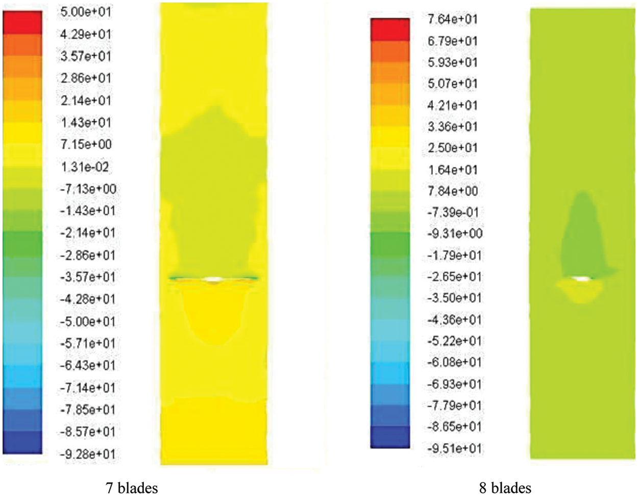
Figure 9: Longitudinal pressure cloud map of the blade

In order to further quantitatively analyze the two types of blades, the solver was used to get the torque of different working conditions. The numerical calculation results are shown in Table 2.

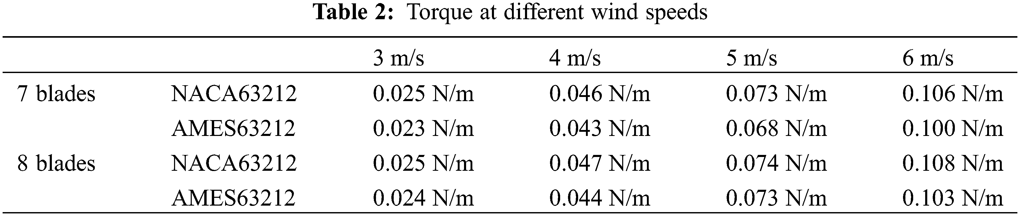
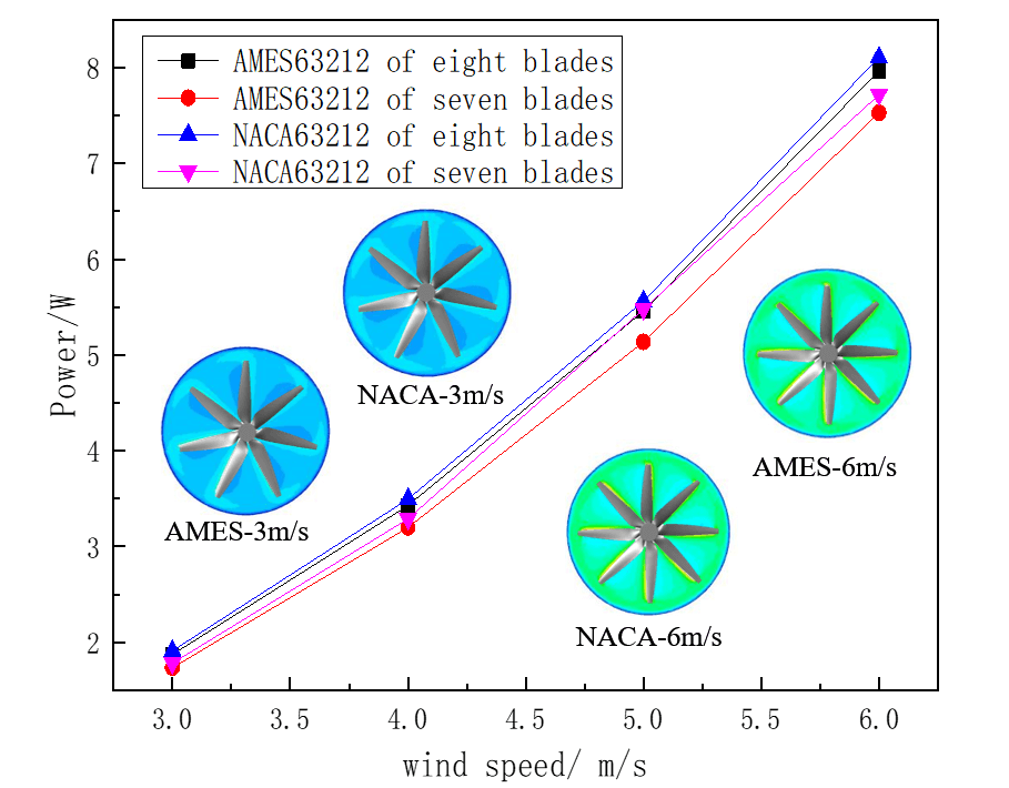
It can be seen from Table 2 that under the same wind speed and the same number of blades, the torque of NACA63212 is greater than that of AMES63212. As the wind speed increases, the torque of both types of blades increases. The torque is converted into turbine power for output eventually. So, based on the information in Table 2 and the wheelbase formula (18), the turbine’s power at different wind speeds can be calculated according to the data in Table 2 while ignoring the conversion efficiency. The calculated results are shown in Fig. 10.

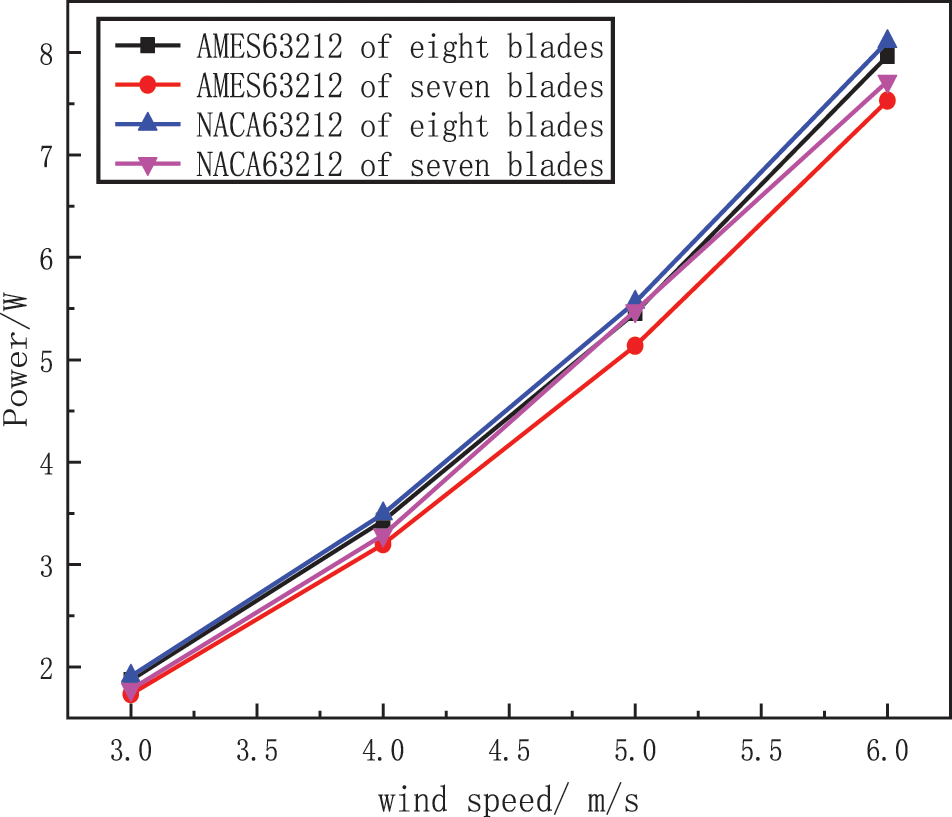
Figure 10: Analysis and comparison of simulation results

P=1000⋅T⋅n9550 (18)

where, P is the output power, W; T is wheelbase, N⋅m; n is speed, r/min.

Fig. 10 shows that the turbine’s power increases with the number of blades and is proportional to the wind speed. Under the same number of blades, the power of the NACA63212 airfoil is higher and the advantage is more obvious compared with AMES63212 when there are seven blades. For the NACA63212 airfoil, the increase in power is smaller as the number of blades increases. For the AMES63212 airfoil, the power increase is larger with the increase in the number of blades, and the power increase is the greatest when the wind speed is 5 m/s.

The impact of various factors on the turbine power is ascertained through the simulation of the two airfoils’ blades, which offers a certain point of reference for the choice and investigation of turbine blades in the future.

5  Conclusion

NACA63212 and AMSE63212 airfoil blades are designed based on Wilson’s theory and mathematical and geometric models. At present, there is little research on the comparison of the two airfoils. The impact of various factors on the turbine power is ascertained through the simulation of the two airfoil blades, which offers a certain point of reference for the choice and investigation of turbine blades in the future. Numerical simulation can draw the effects of blade airfoil, blade number, chord length, torsion angle, and other parameters on turbine power, as well as the pressure and velocity plot distribution at the turbine. The main conclusions are as follows:

(1)   The blade designed by Wilson’s theory can accurately simulate the movement of the blade in the turbine, and the error is within 10% compared with the experimental value.

(2)   The vertical solar power plant’s turbine power increases with the blade number and incoming wind speed. Within the research scope, the power of NACA63212 and AMSE63212 increased by about 6.8% and 5.1% on average with the increase in the number of blades. As the incoming wind speed increase, the power increase rate of the two airfoils is almost the same, about 6.3%.

(3)   For the AMES63212 airfoil, when the wind speed is 5 m/s, the power increases the fastest as the number of blades increases. For NACA63212, when the wind speed is 6 m/s, the power difference between 7-blade and 8-blade turbines is the largest.

(4)   Turbine power is proportional to the chord length and inversely proportional to the torsion angle. Increasing the chord length and reducing the torsion angle within a certain range is beneficial to improving the lift-drag ratio, thereby improving the turbine’s efficiency.

Funding Statement: The authors received no specific funding for this study.

Conflicts of Interest: The authors declare that they have no conflicts of interest to report regarding the present study.

References

    1. Lv, Y., Yang, J., Wang, J. (2020). CFD simulation of a bag filter for a 200 MW power plant. Fluid Dynamics & Materials Processing, 16(6), 1191–1202. DOI 10.32604/fdmp.2020.010302. [Google Scholar] [CrossRef]

    2. Afif, L., Bouaziz, N. (2022). Thermodynamic investigation of a solar energy cogeneration plant using an organic rankine cycle in supercritical conditions. Fluid Dynamics & Materials Processing, 18(5), 1243–1251. DOI 10.32604/fdmp.2022.021831. [Google Scholar] [CrossRef]

    3. Zhou, Y., Wang, L., Gong, Y. Y. (2016). Study on operation mechanism of vertical solar hot-air power station system. Acta Energiae Solaris Sinica, 37(11), 2868–2874. [Google Scholar]

    4. Pasurmarthi, N., Sherif, S. A. (1997). Performance of a demonstration solar chimeny model for power generation, pp. 203–240. California State University, Sacramento, CA, USA. [Google Scholar]

    5. Zhou, Y., Zheng, W. J., Liu, X. H., Li, Q. L. (2011). Study of the heat storage device characteristic in the solar chimney power plant system with vertical collector. Advanced Materials Research, 1159(221), 356–363. DOI 10.4028/www.scientific.net/AMR.221.356. [Google Scholar] [CrossRef]

    6. Zhou, Y., Lu, H. B., Gong, Y. Y. (2015). The design of solar chimney power plant vertical turbine. Journal of Engineering Thermophysics, 36(7), 1542–1546. [Google Scholar]

    7. Felsch, T., Strauss, G., Perez, C., Rego, J. M., Maurtua, I. et al. (2015). Robotized inspection of vertical structures of a solar power plant using NDT techniques. Robotics, 4(2), 103–119. DOI 10.3390/robotics4020103. [Google Scholar] [CrossRef]

    8. Zhou, Y., Gao, B., Dong, H. R., Hao, K. (2016). Design for the turbine of solar chimney power plant system with vertical collector. IOP Conference Series: Earth and Environmental Science, 40(1), 012085. DOI 10.1088/1755-1315/40/1/012085. [Google Scholar] [CrossRef]

    9. Wang, Q., Chen, X. T., Huang, P., Gan, D., Zeng, L. L. et al. (2020). Comparison of aerodynamic performance of two airfoils for vertical-axis wind turbines. Renewable Energy, 38(2), 199–204. [Google Scholar]

  10. Jia, S. L., Wang, Z. Y., Qu, Y. C., Liu, K., Zhou, X. Y. et al. (2019). Wind turbine blade structure design and numerical simulation. Machine Tool & Hydraulics, 47(11), 168–172. [Google Scholar]

  11. Wu, Y. j., Yang, Y. (2020). Influence of different turbulence models on aerodynamic performance parameters of wind turbine blade airfoil. Solar Energy, 8, 36–40. [Google Scholar]

  12. Wu, Y. J., Yang, Y. (2020). Numerical calculation of aerodynamic performance of wind turbine blade airfoil based on fluent. Energy Saving, 39(1), 96–100. [Google Scholar]

  13. Xu, X. W., Sun, H. H., Hua, G. S., Wu, X. L. (2019). Optimum design of wind turbine blade parameters based on genetic algorithm. Journal of Nanjing University of Technology, 41(4), 508–513. [Google Scholar]

  14. Yu, H. W., Xu, C. Y. (2018). Analysis of aerodynamic performance of wind turbine blade structure based on dove-like airfoil. Journal of Changchun University of Science and Technology, 41(1), 95–100. [Google Scholar]

  15. Zhao, Z. M., Chen, N. Z. (2022). Acoustic emission based damage source localization for structural digital twin of wind turbine blades. Ocean Engineering, 265. DOI 10.1016/j.oceaneng.2022.112552. [Google Scholar] [CrossRef]

  16. Lazzerini, G., Coiro, D. P., Troise, G., D’Amato, G. (2022). A comparison between experiments and numerical simulations on a scale model of a horizontal-axis current turbine. Renewable Energy, 190, 919–934. DOI 10.1016/j.renene.2022.03.162. [Google Scholar] [CrossRef]

  17. Gang, H., Bo, Q., Chen, H. X. (2022). Parametric design and optimization of tubular turbine runner blades. Journal of Mechanical & Electrical Engineering, 39(6), 820–825. [Google Scholar]

  18. Fan, X. F., Yang, P. F., Xu, B. H., Song, C. S. (2021). Design and analysis of axial flow impeller based on CFD. Digital Manufacture Science, 19(3), 192–197. [Google Scholar]

  19. Li, P. C., Zhou, Y., Gao, Y., Zhang, S. K. (2021). Airfoil design and performance analysis of wind turbine blades. Journal of Qingdao University of Science and Technology, 42(5), 94–102. [Google Scholar]

  20. Mei, Z. H., Liu, S. J., Deng, W. W. (2021). Finite element simulation of aeroengine turbine blade based on ANSYS. Mechanical & Electrical Engineering Technology, 50(11), 33–36. [Google Scholar]

  21. Wei, Y. C., Wang, H. Y. (2017). Performance study of an aero-engine turbine blade in service. Computer & Digital Engineering, 45(7), 1243–1248. [Google Scholar]

  22. Lu, Y. K., Yang, J. X. (2019). Experimental study on the influence of blade number on the aerodynamic performance of SCPPVC air turbine. Science, Technology and Engineering, 19(22), 169–173. [Google Scholar]

  23. Ming, T. Z., Liu, W., Xu, G. L. (2006). Analytical and numerical investigation of the solar chimney power plant systems. International Journal of Energy Research, 30(11), 861–873. DOI 10.1002/(ISSN)1099-114X. [Google Scholar] [CrossRef]

  24. Sun, W. (2012). Key structure optimization design of small wind turbine (Master Thesis). Suzhou University, Suzhou, China. [Google Scholar]

  25. Rabehi, R., Chaker, A., Ming, T. Z., Gong, T. R. (2018). Numerical simulation of solar chimney power plant adopting the fan model. Renewable Energy, 126, 1093–1101. DOI 10.1016/j.renene.2018.04.016. [Google Scholar] [CrossRef]

  26. Liu, T. R., Chang, L. (2018). Vibration control of wind turbine blade based on data fitting and pole placement with minimum-order observer. Shock and Vibration, 2018, 5737359. DOI 10.1155/2018/5737359. [Google Scholar] [CrossRef]

  27. Hao, K. (2018). Optimal design of SCPPVC system double rotor air turbine (Master Thesis). School of Mechanical and Electrical Engineering Department, Qingdao University of Science and Technology, China. [Google Scholar]

  28. Wahba, E. M. (2022). Derivation of the differential continuity equation in an introductory engineering fluid mechanics course. International Journal of Mechanical Engineering Education, 50(2), 538–547. DOI 10.1177/03064190211014460. [Google Scholar] [CrossRef]

  29. He, D. X., Wang, X. D., Liu, J., Guo, C. Y., Li, H. K. et al. (2022). Based on SST K − ω research on piston wind effect of lift shaft for turbulence model. Nonferrous Metals Engineering, 12(8), 149–158. [Google Scholar]