
 Submit a Paper
 Propose a Special lssue
 Open Access
ARTICLE

A Dynamic Plunger Lift Model for Shale Gas Wells
1 Petroleum Engineering Institute of Yangtze University, Wuhan, 430100, China
2 Laboratory of Multiphase Pipe Flow, Gas Lift Innovation Center, China National Petroleum Corp., Yangtze University, Wuhan, 430100, China
3 Key Laboratory of Drilling and Production Engineering for Oil and Gas, Wuhan, 430100, China
4 Sichuan Shale Gas Exploration and Development Limited Liability Company, Chengdu, 640000, China
5 Sichuan Changning Gas Development Company, PetroChina Southwest Oil & Gas Field Company, Chengdu, 610051, China
6 Oil and Gas Technology Research Institute of Changqing Oilfield Company, PetroChina, Xi’an, 710018, China
* Corresponding Author: Wei Luo. Email:
Fluid Dynamics & Materials Processing 2023, 19(7), 1735-1751. https://doi.org/10.32604/fdmp.2023.025681
Received 26 July 2022; Accepted 08 November 2022; Issue published 08 March 2023
 View Full Text
 Download PDF
Abstract
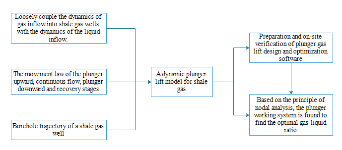
At present, the optimization of the plunger mechanism is shale gas wells is mostly based on empirical methods, which lack a relevant rationale and often are not able to deal with the quick variations experienced by the production parameters of shale gas wells in comparison to conventional gas wells. In order to mitigate this issue, in the present work, a model is proposed to loosely couple the dynamics of gas inflow into shale gas wells with the dynamics of the liquid inflow. Starting from the flow law that accounts for the four stages of movement of the plunger, a dynamic model of the plunger lift based on the real wellbore trajectory is introduced. The model is then tested against 5 example wells, and it is shown that the accuracy level is higher than 90%. The well ‘switch’, optimized on the basis of simulations based on such a model, is tested through on-site experiments. It is shown that, compared with the original switch configuration, the average production of the sample well can be increased by about 15%.Graphic Abstract
Keywords
Nomenclature
| | gas well gas production, 104 m3/d |
| | gas well liquid production, m3/d |
| | as well exponential equation coefficient, 104 m3/d/MPa2n |
| | gas well fluid production index, m3/d/MPa |
| | quality of plunger, kg |
| | quality of liquid column, kg |
| | weight acceleration, kg ⋅ m/s2 |
| | acceleration of the plunger motion when the plunger is in the first segment, m/s2 |
| | lower end pressure when plunger is in section, MPa |
| | pressure at the top of the plunger and liquid column when the plunger is in the first section, MPa |
| | tubing cross section area, m2 |
| | friction resistance between the liquid column and the tubing when it is in the first stage, N |
| | friction resistance between plunger and tubing in stage, N |
| | friction coefficient between plunger, liquid column, and tubing |
| | correction factor of friction coefficient between plunger and tubing |
| | density of liquids, kg/m3 |
| | average plunger density, kg/m3 |
| | upward speed of plunger and liquid column, m/s |
| | length of liquid column, m |
| | length of plunger, m |
| | tube diameter, m |
| | quality of the upper liquid when there is still a section of the upper liquid column on the plunger, kg |
| | length of liquid segment on plunger, m |
| | the amount of liquid flow through the wellhead throttle valve when the liquid column on the plunger is left with stage i, m3/d |
| | the liquid flow coefficient through the wellhead throttle valve, 0.987 |
| | wellhead pipeline diameter, m |
| | gas mass change in the annulus of the oil jacket and in the oil pipe at t moments, kg |
| | gas mass produced by strata at t time, kg |
| | gas quality discharged through wellhead throttle valve at t times, kg |
| | buoyancy exerted by the plunger dropping in the air column at t moment, N |
| | friction resistance of a plunger dropping in the air column at t moment, N |
| | volume of plunger, m3 |
| | the coefficient of resistance of the plunger falling in the gas column, dimensionless |
| | density of gas, kg/m3 |
| | drop speed of plunger in gas column, m/s |
| | buoyancy exerted by the plunger dropping in the liquid column at t moment, N |
| | friction resistance of a plunger dropping in the liquid column at t moment, N |
| | resistance factor, dimensionless, for plunger falling in liquid column |
| | drop speed of plunger in liquid column, m/s |
The plunger drainage gas lift process is a drainage gas recovery method that uses the formation energy to push the plunger in the tubing to reciprocate up and down to discharge the wellbore liquid by intermittently switching wells for natural gas development. The plunger drainage gas recovery process is one of the main drainage and recovery technology measures in the current gas well production. The research on the optimal design of the plunger gas lift production working system is of great significance to ensure the efficient development of gas wells and improve the work efficiency of field managers. Nonetheless, since large-scale fracturing is commonly used in the current large-scale development and application of shale gas fields, liquid production is relatively large in the early stage of development. Then the liquid production continues to decline slowly, and the production parameters change relatively faster than in conventional gas wells. The gas lift working system will become unsuitable at present. It is difficult for the on-site plunger gas to lift well to be in an optimal production state, and timely adjustment is required to ensure the long-term and efficient development of the plunger gas lift well. The laws are complex, and the structure of horizontal wells is complex, so there is still a lack of suitable design and optimization methods. Although the related research on plunger gas lift has been started at an early stage, most of them are carried out on oil wells, and there are few pieces of research on gas wells.
In the 1960s, Foss et al. [1] established the static operation model of plunger gas lift for the first time based on the field data of many gas wells in gas fields, and drew a series of more general plunger lift dynamic curves. In 1980, Abercrombie [2] established and improved the static model with a large amount of plunger drop velocity data. In 1982, Lea [3] established the first dynamic model, the essence of which is to describe the change of the speed of the plunger with time and depth. In 1985, Mower et al. [4] established a dynamic model similar to the Lea model by introducing the liquid loss term based on field data. In 1987, Beeson et al. [5] finally obtained a nomogram representing the characteristics of a plunger gas lift by analyzing some data. In 1994, Marcano et al. [6] established a dynamic model of plunger gas lift considering the fluid loss during the lifting process. In 1995, Baruzzi et al. [7] proposed a dynamic model that simply describes the plunger gas lift based on experiments. In 1997, Gasbarri et al. [8] further improved the plunger lift dynamic model. The model presents a more complete description of the discharge system. The simulation results also show that the discharge system directly affects the casing pressure, liquid column size, and rising velocity.
In 2000, Maggard et al. [9] established a dynamic model of a plunger gas lift that can be used in tight gas wells. In 2008, Chava et al. [10] proposed a new method to simulate the lift of the plunger, which can more accurately reflect the actual dynamics of the plunger. In the same year, Tang et al. [11,12] proposed a new model that describes the movement of the plunger, which took into account the effects of changes in oil jacket pressure, fluid accumulation, liquid fallback, and plunger resistance. In 2010, Sask et al. [13] explored the effects of wellbore trajectory and fluid retention on the plunger performance through examples. In 2011, Kravits et al. [14] conducted a theoretical study on applying the plunger gas lift drainage gas recovery technology in horizontal wells, and proved that the plunger gas lift technology can be applied in large inclination angles of horizontal wells.
In 2015, Nascimento et al. [15] studied three shale gas wells with different trajectories. Its findings guide optimizing horizontal shale well startups and designing optimal shale well trajectories for plunger lift operations. It highlights the role of transient simulations in the planning stage of shale development. In 2017, Arun et al. [16] established the first instance of modeling complex system of plunger lift using a standard hybrid system model framework. The resulting model is used to present insight into plunger lift operation, including an efficient simulation of multiple plunger cycles and analysis of the effect of uncertainties on the well behavior. In 2021, the new model proposed by Zhao et al. [17] can obtain the basic parameters of the plunger lift cycle. And calculate the hydrocarbon mixture properties in gas wells through component models, thus providing more accurate and reasonable predictions of tubing and casing pressures.
It can be seen that the research on plunger gas lift has gradually changed from the early empirical model to the theoretical model, from application in oil wells to application in oil and gas wells, from application in vertical wells to application in complex wells such as inclined wells and horizontal wells. The research has become more and more abundant and gradually become better. However, for the shale gas horizontal wells that have been completed, the well structure is complex, and the production conditions are complex and changeable. There are few studies that require long-term and efficient development, and few are feasible after on-site scale verification. Given this, it is necessary to conduct research that is more in line with the production gas-liquid inflow dynamics of shale gas wells and the corresponding research on the design method of the plunger gas lift simulation model to guide the development of a more reasonable well opening and closing work system on site, and ensure the rapid development and efficient operation of shale gas fields.
1.1 Gas-Liquid Inflow Dynamic Method for Shale Gas Wells
Different from conventional reservoir rocks, shale reservoirs have the characteristics of small pore throats (micron-nanoscale), complex and diverse pore structures, and strong heterogeneity, which leads to the influence of pore structure on shale gas storage performance and fluid seepage characteristics are more obvious [18]. Based on the gas-bearing and gas-producing test data of shale gas wells, some scholars divide shales into three types by electrical characteristics: type I low resistance (less than 1
In general, the geological conditions and development techniques of shale oil reservoirs are quite different from those of conventional oil reservoirs. The geological characteristics of shale oil reservoirs are complex, and the storage space has multi-scale characteristics, including nano-pores, micro-pores, micro-cracks, and fractures; shale has low porosity and extremely low permeability. Shale oil wells generally have no natural productivity and need to be developed by horizontal wells and large-scale hydraulic fracturing. In addition, shale oil passes through natural fractures and artificial fractures step by step, making the process more complicated. This differs from the theory of conventional oil and gas reservoirs [20–22].
Therefore, in actual production, conventional productivity prediction methods cannot be used, and it is urgent to determine the production model of shale gas through more in-depth research to provide a foundation for the study of the flow state in the shale gas wellbore and the theoretical study of the prediction of fluid accumulation.
In this paper, through the analysis of a large number of field production data of horizontal gas wells, it is found that the ratio of water production to gas production in horizontal gas wells is not constant. Among them, the changing law of water production is complex and changeable, which is affected by the initial flow back rate. It is also related to the location of the pressure fractures flowing into the reservoir and the size of the gas production in the reservoir. Small, the fluid production in the middle and late drainage process mostly shows a fluctuating pattern of high and low (the production fluid flows out of the horizontal wellbore one by one). The variation law of gas production is slightly simpler than that of water production, and the overall performance trend is consistent with that of water production. The initial gas production is large, and the gas production gradually decreases as the production time becomes longer. In a relatively short period of time, gas production showed a slow decline, and the change rule of fluctuating highs and lows was not obvious, which was mainly affected by water output. The proportion of gas-liquid inflow is not necessarily fixed. Therefore, this paper loosely couples gas inflow dynamics and liquid inflow dynamics in shale gas wells, and each gas and liquid follows its own inflow dynamic equation. Among them, the dynamic inflow equation of formation gas production can use the binomial equation or other gas well productivity prediction methods such as the exponential equation. Taking the exponential equation as an example, the equation is [23]:
The dynamic inflow equation of formation fluid can be a fluid production exponential equation, such as the Vogel equation, Fetkovich equation, Petrobras equation, etc. Taking the fluid production exponential equation as an example, the equation is:
where
1.2 Plunger Gas Lift Design Method
Usually, the entire movement process of the plunger gas lift is divided into four stages: the plunger ascending stage, the freewheeling production stage, the plunger descending, and the pressure recovery stage. The force analysis of each movement stage can be obtained separately according to the momentum conservation equation.
When the plunger and the liquid column do not reach the wellhead, the following Fig. 1 is shown:
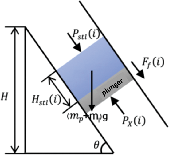
Figure 1: The plunger goes up and does not reach the wellhead
During the process of plunger rise, the whole well segment is divided into i segments, and each segment is subjected to force analysis concerning the well depth trajectory as follows:
Force analysis is performed on the plunger and the upper fluid segment. As shown in Fig. 1, the forces acting on the plunger are: pressure
Among them, the frictional resistance between the plunger and the tubing is calculated, and the frictional resistance between the plunger and the tubing is calculated by the method of liquid phase friction resistance. However, in the actual simulation process, it is found that the friction resistance of the plunger in the large inclined well or horizontal well is a factor that cannot be ignored in the actual production, but the existing literature has not conducted theoretical research on the friction coefficient of the plunger. Therefore, the coefficient k is added to the original liquid column friction resistance calculation method by the same type of analogy. The specific k-value is calculated by inversion from the actual data of the site during the simulation optimization process to obtain the piston friction coefficient under different well types.
where
When the liquid column reaches the wellhead, Fig. 2 below shows it:
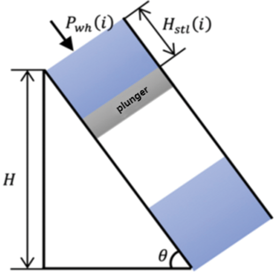
Figure 2: Diagram of the plunger going up to the wellhead
When the upper liquid segment of the plunger reaches the wellhead, the fluid segment begins to drain out of the well bore. This stage starts with the liquid slug in the upper part of the plunger reaching the wellhead. When all the liquid segments in the upper part of the plunger are discharged from the wellhead, the discharging stage ends, and the distance of movement is equal to the height of the liquid segment in the upper part of the plunger. The liquid column height on the top of the plunger is evenly divided into n segments, making i = n, n − 1,
The force analysis is carried out on the plunger and the upper non-drained liquid section, which is the same as Fig. 2. The difference is that as the liquid is drained, the length of the liquid section decreases continuously, and the gravity and friction generated by the liquid column change. In this stage, the liquid in the upper part of the plunger reaches the wellhead position, where the wellhead oil pressure is equal to the surface pressure of the liquid in the upper part of the plunger, that is:
During this stage, the liquid in the upper part of the plunger is continuously discharged, and the liquid quality in the upper part of the plunger becomes:
Assuming that the well head has a throttle valve, with the expansion of the annulus air body and the formation produced gas and liquid flowing into the tubing, pushing the plunger upward, the liquid slug above the plunger gradually discharges from the well head, and the liquid quality discharged through the throttle valve is:
Among them, the size of fluid flow
where
When the plunger reaches the wellhead and is captured by the trap, the wellhead enters the continuous flow production stage while the wellhead is still open for production.
The continuous flow production stage means that after the liquid slug has completely entered the production pipeline, the plunger stays in the wellhead catcher position and continues to open the well until the well closes, as shown in Fig. 3. The stage is divided into n segments according to the continuous flow production time, making t = 1, 2, 3,
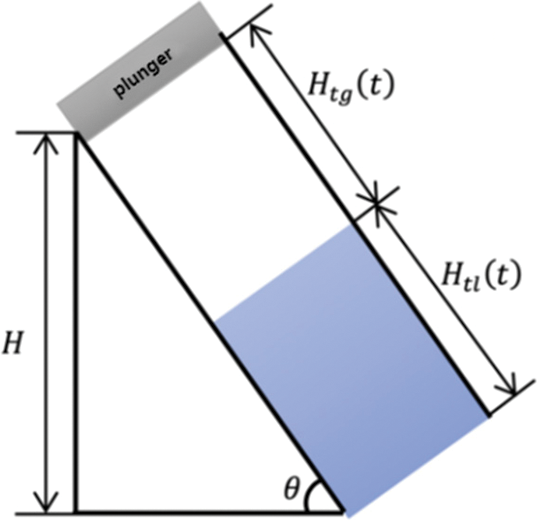
Figure 3: Freewheeling production stage
According to the law of gas mass conservation, the gas mass produced by the wellhead is determined by
where
During plunger descent, the whole well segment is divided into i segments, and each segment is subjected to force analysis regarding the well depth trajectory as follows: The force analysis of the plunger is carried out. As shown in Fig. 4, the force acting on the plunger during the plunger falling is: The gravity
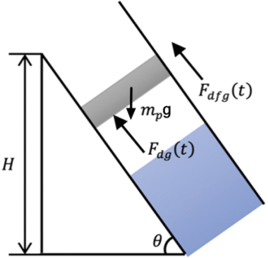
Figure 4: The plunger goes down in the gas
where:
where
The force analysis of the plunger is carried out. As shown in Fig. 5, the force acting on the plunger during the falling of the plunger in the liquid column is: the gravity M of the plunger itself, the buoyancy F of the plunger when it falls in the liquid column, and the friction resistance G of the plunger when it falls in the liquid column. Using Newton’s second law are:
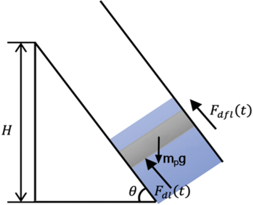
Figure 5: The plunger descends in the liquid
where:
where
After shut-in, as the gas and liquid produced by the formation continuously flow into the wellbore, it enters the pressure recovery stage. According to the shut-in time, this stage is divided into N sections, t = 1, 2, 3, …, N represents the state of the plunger well at time t.
During shut-in, the gas and water produced by the formation enters the tubing and casing at the same time, causing changes in the casing pressure. It is assumed that the average cross-sectional area of gas and liquid produced by the formation enters into the tubing and casing annulus in equal proportions, which causes changes in the liquid level, oil pressure, and casing pressure of the tubing and the annulus at the same time. The gas and liquid produced by the formation are related to the bottom-hole flow pressure in any period of time, and are calculated by the calculation method in Section 1.1. The initial value of the pressure and their respective volumes at the beginning of the recovery stage of the tubing and casing annulus (considering the volume of liquid and the volume lost in the casing entering the tubing in the previous cycle), after the recovery period, the respective pressures of the tubing and the casing annulus and their respective volumes. The size of the volume can be calculated from the conservation of mass and the state of the gas.
According to the principle of mass conservation, the gas mass
Before the implementation of the plunger gas lift, it is necessary to optimize the design of its process parameters. The main working parameters of the optimized design include the cycle time of the opening well, the cycle time of the closing well, minimum casing pressure, maximum casing pressure, single-cycle lifting fluid volume, and the number of plunger cycles. Based on the principle of node analysis, the specific flow chart of the plunger gas lift design under a certain switching time working system is shown in Fig. 6.
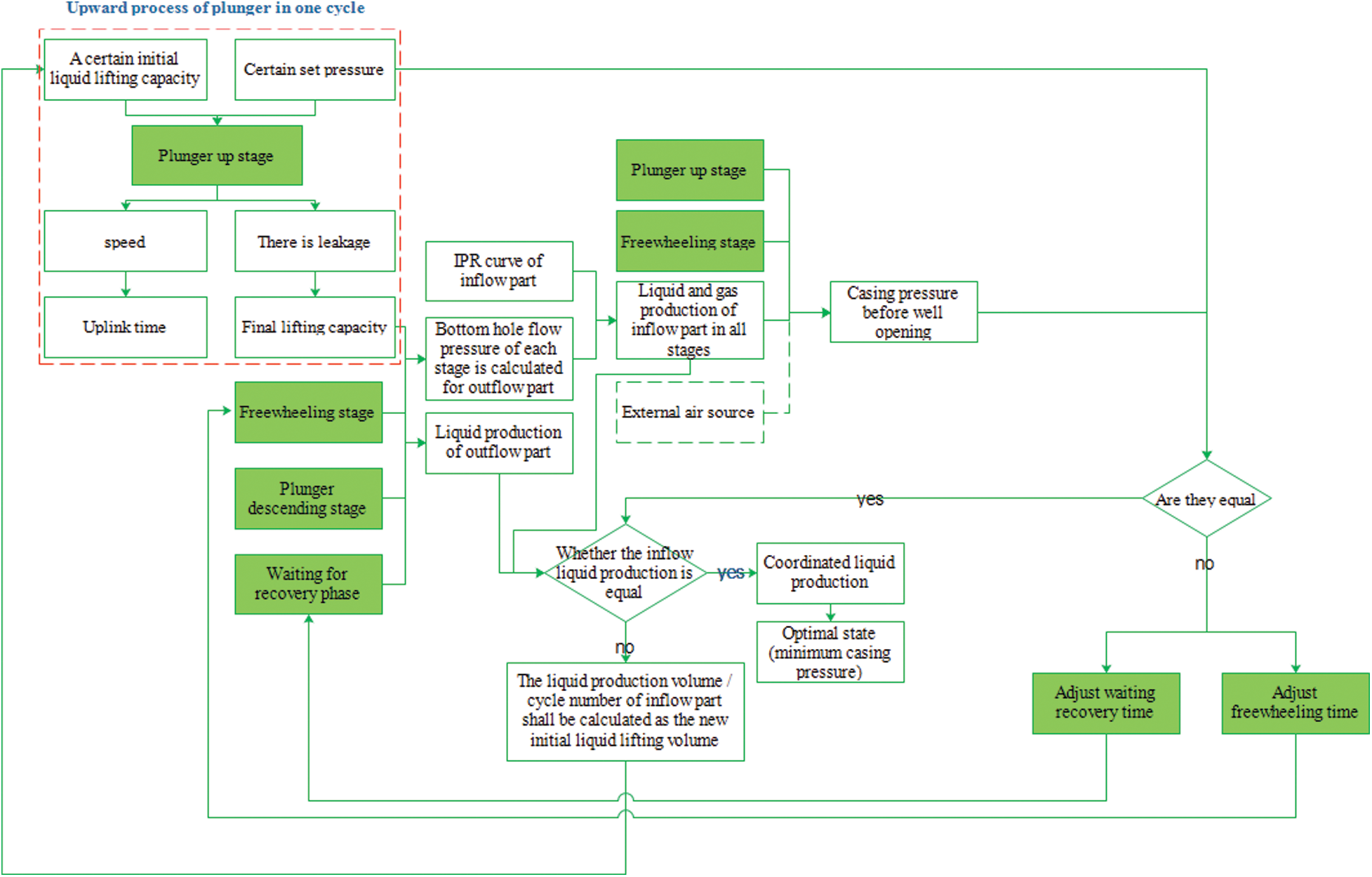
Figure 6: Fixed-time mode (Fixed switching time or the freewheeling recovery time) plunger gas lift optimization design flow chart
The plunger gas lift is often in a non-optimal production state during the production process, as shown in Fig. 7. The optimization of the plunger gas lift production process is mainly to optimize the plunger gas lift working system, so that the plunger gas lift is always in a high-efficiency state, that is, to obtain a lower average bottom hole flow pressure and high gas production or liquid discharge as much as possible.
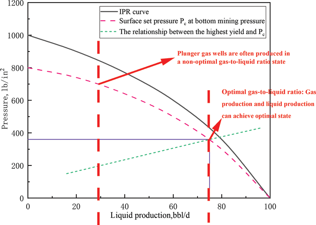
Figure 7: The state in which the piston gas lift is produced
Therefore, the optimization of the plunger gas lift production process is actually: the search process of the minimum coordinated production casing pressure. In view of this, a basic optimization (intelligent optimization) strategy in the time optimization mode is proposed, and the detailed optimization process is shown in Fig. 8 below.
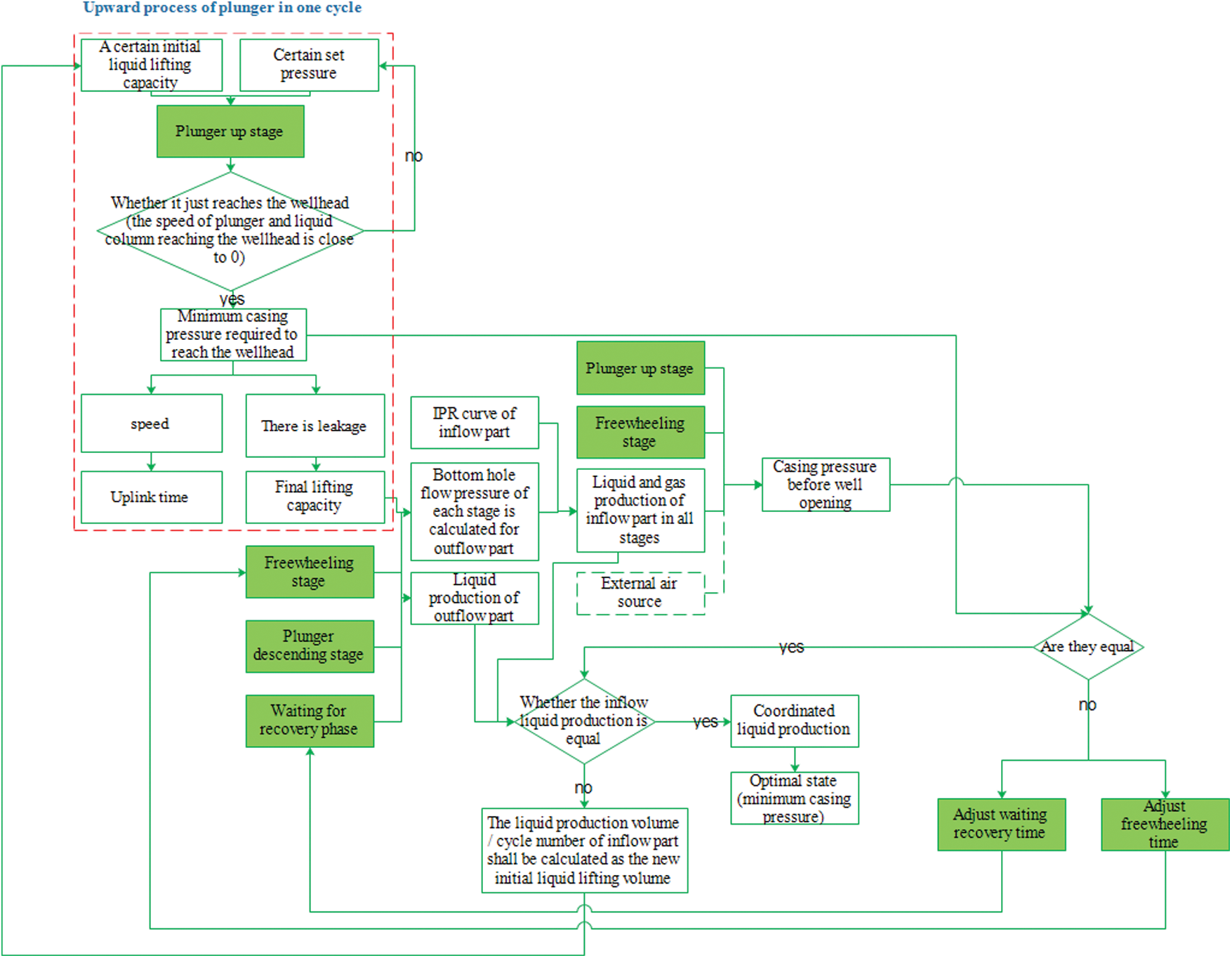
Figure 8: Fixed-time mode (Fixed switching time or freewheeling recovery time) plunger gas lift production system optimization flow chart (Time mode basic optimization strategy)
2 Validation of Calculation Examples and Optimization of Work System
2.1 Example 1 Well Simulation Calculation Verification
2.1.1 Example 1 Well Theory Model Validation
The specific parameters of Well Example 1 is shown in Table 1, the software simulation results are shown in Fig. 9, and the software simulation optimization results are shown in Fig. 10.

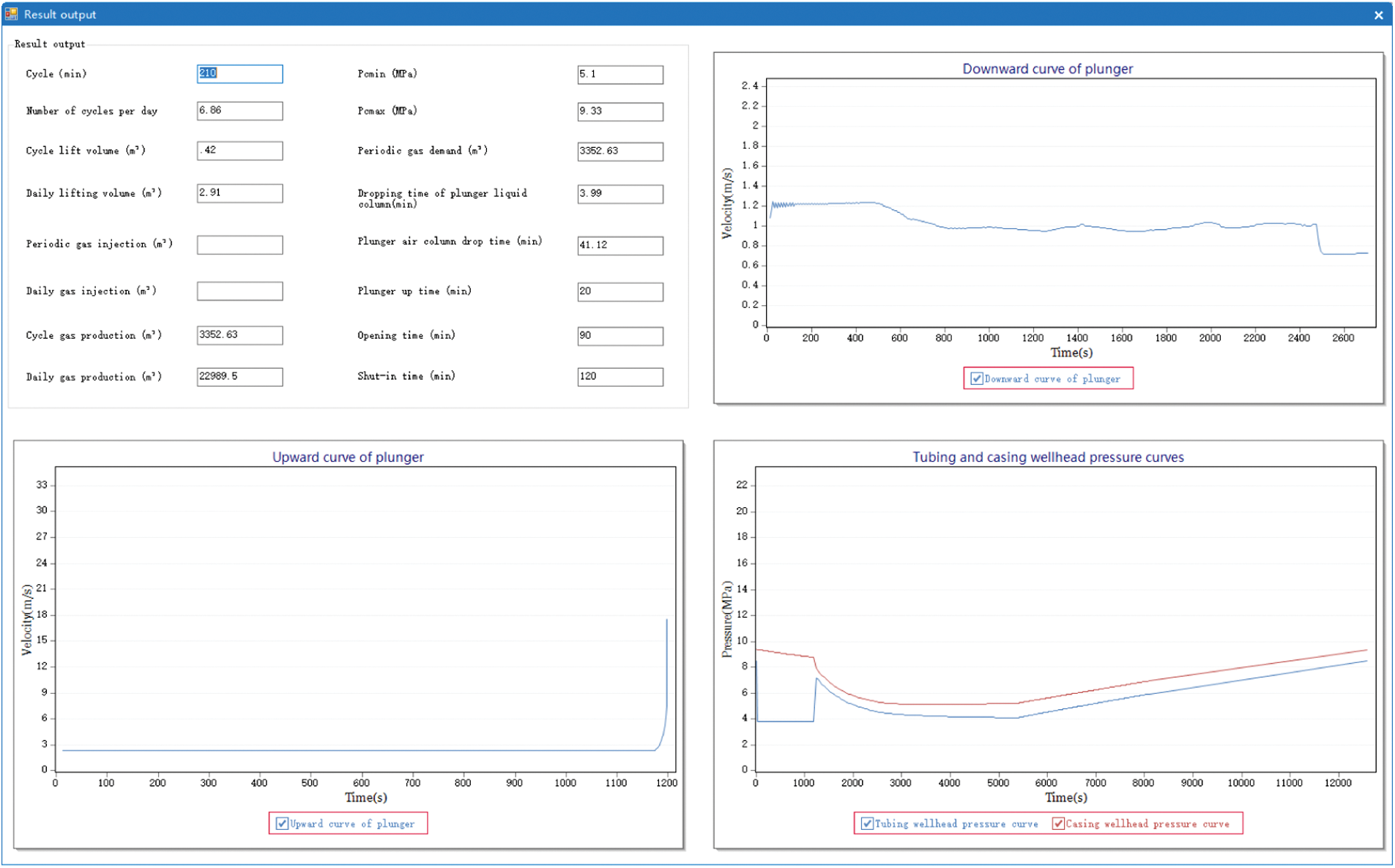
Figure 9: Theoretical simulation results of Well 1
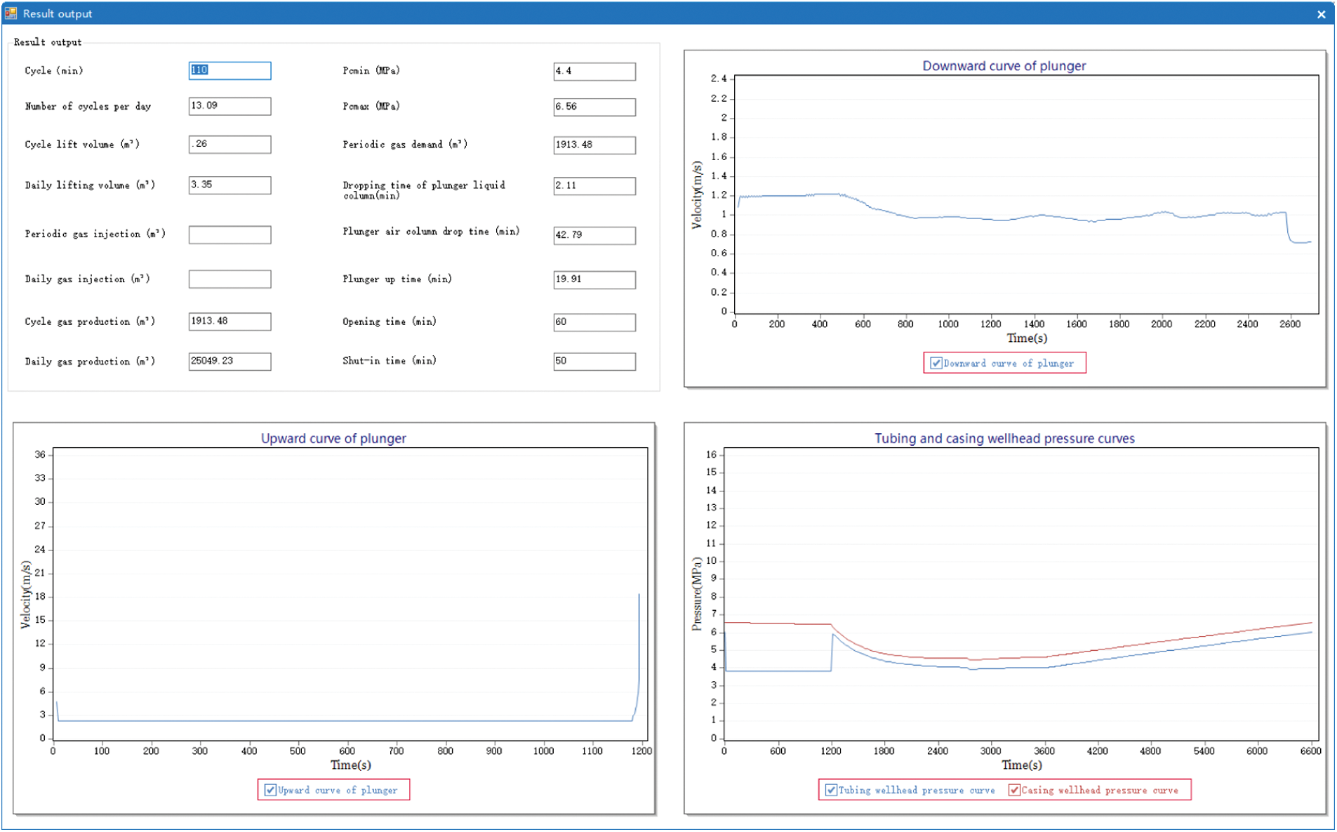
Figure 10: Theoretical simulation and optimization results of Well 1
The software simulation specific data and optimization data are shown in Table 2:

2.1.2 Field-Instance Applications
The measured data verification results are shown in Table 3:

According to the recommended working system of software simulation optimization and the actual situation of the field, the working system of the example well is adjusted. The specific comparison value is the average value of the production data of a period of relatively stable production before adjustment and the average value of a period of stable production after adjustment. The time period is generally one to two weeks. The specific adjustment effects are shown in Table 4, Figs. 11 and 12 are the daily water/gas comparison diagrams before and after the adjustment of Well 1 and Well 2.

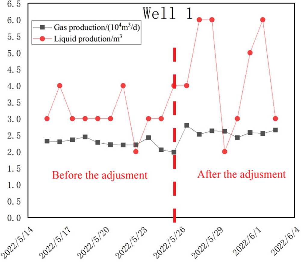
Figure 11: Well 1 adjustment before and after comparison results
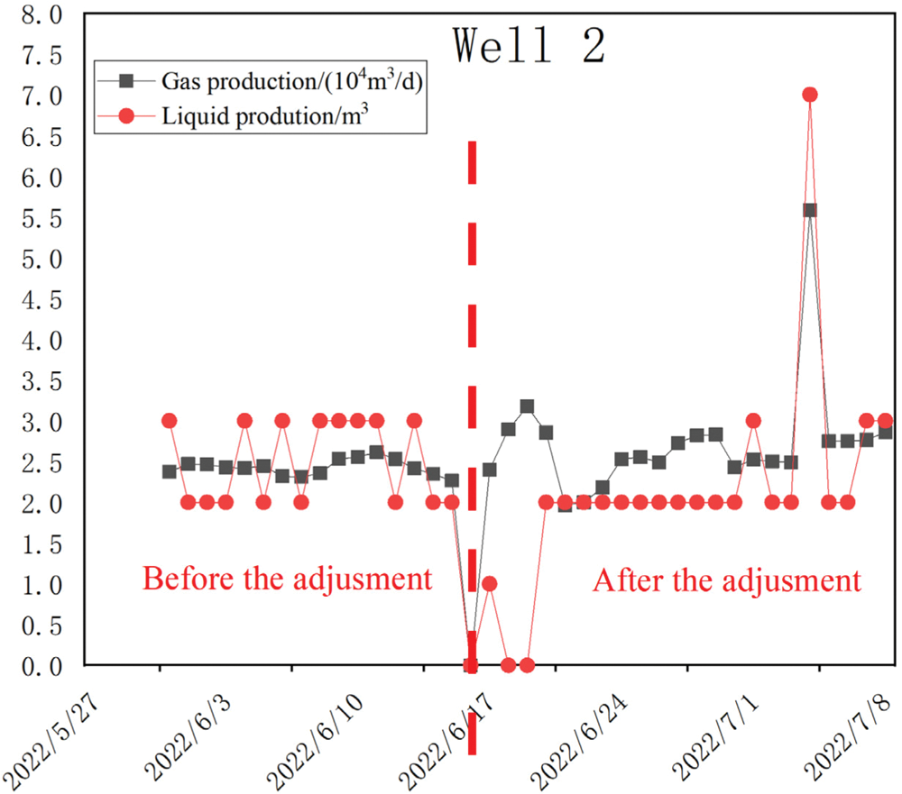
Figure 12: Well 2 adjustment before and after comparison results
For the shale gas horizontal wells that have been completed, the well structure is complex, and the production conditions are complex and changeable. There are few studies that require long-term and efficient development, and there are few comparisons with on-site verification. A method is proposed to loosely couple the gas inflow dynamics and liquid inflow dynamics of shale gas wells, and the gas and liquid follow their respective inflow equations. Combined with the four motion laws of the plunger, a plunger gas lift considering the real wellbore trajectory is established. Dynamic simulation model. On this basis, software development is carried out. It is verified by field example verification analysis, which shows that:
(1) The model can reflect the relationship between the residence time at the wellhead (after-flow time) and the gas production during the after-flow process at the wellhead, and can describe the relationship between the upward and downward velocity of the plunger and the casing pressure and time, following the conservation of mass and momentum Theorem, forming a strict theoretical closed loop.
(2) Based on the same production data and parameters, such as the up and down time of the plunger, the simulated output is compared with the actual output through the simulation calculation, and the error is within 10%. It shows that the plunger gas lift design under the simulation model has a high accuracy.
(3) The actual gas production can be increased by about 15% after adjusting the well switching time through simulation optimization and performing on-site verification. It shows that the established simulation model and the developed software have practical guiding significance for the actual design optimization in the field.
Acknowledgement: Thanks for Luo Wei, of the corresponding author for the article.
Funding Statement: The authors would like to acknowledge the National Natural Science Fund Project (62173049) for Key Project and the Open Fund Project “Study on Transient Flow Mechanism of Fluid Accumulation in Shale Gas Wells” of the Sinopec Key Laboratory of Shale Oil/Gas Exploration and Production Technology.
Conflicts of Interest: The authors declare that they have no conflicts of interest to report regarding the present study.
References
1. Foss, D. L., Gaul, R. B. (1965). Plunger-life performance criteria with operating experience–Ventura avenue field. Drilling and Production Practice. American Petroleum Institute. API-65-124. [Google Scholar]
2. Abercrombie, B. (1980). Plunger lift. In: The technology of artifificial lift methods, pp. 483–518. USA: Penn Well Publishing Co. [Google Scholar]
3. Lea, J. F. (1982). Dynamic analysis of plunger lift operations. Journal of Petroleum Technology, 34(11), 2617–2629. https://doi.org/10.2118/10253-PA [Google Scholar] [CrossRef]
4. Mower, L. N., Lea, J. F., Beauregard, E., Ferguson, P. L. (1985). Defifining the characteristics and performance of gas-lift plungers. 60th Annual Technical Conference and Exhibition of the Society of Petroleum Engineers, Las Vegas. NV. SPE14344. [Google Scholar]
5. Beeson, C. M., Knox, D. G., Al-Bassam, M., Chilingarian, G. V. (1987). Plunger lift. Developments in Petroleum Science, 19, 467–530. https://doi.org/10.1016/S0376-7361(08)70542-9 [Google Scholar] [CrossRef]
6. Marcano, L., Chacin, J. (1994). Mechanistic design of conventional plunger lift installation. SPE Advanced Technology Series, 2(1), 15–24. https://doi.org/10.2118/23682-PA [Google Scholar] [CrossRef]
7. Baruzzi, J., Alhanati, F. (1995). Optimum plunger lift operation. Production Operations Symposium, Oklahoma City, Oklahoma, USA. https://doi.org/10.2118/29455-MS [Google Scholar] [CrossRef]
8. Gasbarri, S., Wiggins, M. L. (1997). A dynamic plunger lift for gas wells. SPE Production Operations Symposium, Oklahoma City, Oklahoma, USA. https://doi.org/10.2118/37422-MS [Google Scholar] [CrossRef]
9. Maggard, J. B., Wattenbarger, R. A., Scott, S. L. (2000). Modeling plunger lift for water removal from tight gas wells. 2000 SPE/CERI Gas Technology Symposium, Calgary, Alberta Canada. SPE59747. [Google Scholar]
10. Chava, G. K., Falcone, G., Teodoriu, C. (2008). Development of a new plunger-lift model using smart plunger data. 2008 SPE Annual Technical Conference and Exhibition, Denver, Colorado, USA. SPE115934. [Google Scholar]
11. Tang, Y. L., Liang, Z. (2008). A new method of plunger lift dynamic analysis and optimal design for gas well deliquifification. 2008 SPE Annual Technical Conference and Exhibition, Denver, Colorado, USA. SPE116764. [Google Scholar]
12. Tang, Y. L. (2009). Plunger lift dynamics characteristics in single well and network system for tight gas well deliquifification. 2009 SPE Annual Technical Conference and Exhibition, New, Orleans, Louisiana, USA. SPE124571. [Google Scholar]
13. Sask, D., Kola, D., Tuftin, T. (2010). Plunger lift optimization in horizontal gas wells: Case studies and challenges. Canadian Unconventional Resources & International Petroleum Conference, Calgary, Alberta, Canada. SPE137860. [Google Scholar]
14. Kravits, M., Frear, R., Bordwell, D. (2011). Analysis of plunger lift applications in the marcellus shale. SPE Annual Technical Conference and Exhibition, Denver, Colorado, USA. SPE147225. [Google Scholar]
15. Nascimento, C. M., Becze, A., Virues, C. J., Wang, A. (2015). Using dynamic simulations to optimize the start-up of horizontal wells and evaluate plunger lift capability: Horn river shale gas trajectory-based case study. SPE Western Regional Meeting, Garden Grove, California, USA. SPE174053. [Google Scholar]
16. Arun, G., Niket, S. K., Naresh, N. N. (2017). Dynamic plunger lift model for deliquification of shale gas wells. Computers & Chemical Engineering, 103, 81–90. https://doi.org/10.1016/j.compchemeng.2017.03.005 [Google Scholar] [CrossRef]
17. Zhao, Q., Zhu, J., Cao, G., Zhu, H., Zhang, H. (2021). Transient modeling of plunger lift for gas well deliquifification. SPE Journal, 26(5), 1–20. https://doi.org/10.2118/205386-PA [Google Scholar] [CrossRef]
18. Dianfa, D., Yaozu, Z., Lina, Z., Xin, L., Mengran, X. (2021). Research progress and prospect of seepage mechanism in shale gas reservoirs.Unconventional Oil & Gas, 2021, 8(3), 1–9. https://doi.org/10.19901/j.fcgyq.2021.03.01 [Google Scholar] [CrossRef]
19. Lin, M., Xiani, J., Jinsong, G. (2022). Analysis of logging characteristics of high quality shale gas reservoirs. Reservoir Evaluation and Development, 2022, 12(3), 445–454. [Google Scholar]
20. Yandong, G. (2018). Capacity forecasting method of shale gas wells based on mass balance equation. China Mining Magazine, 27(6), 153–159. [Google Scholar]
21. Fetkovich, M. J., Fetkovich, E. J., Fetkovich, M. D. (1997). Useful concepts for decline curve forecasting, reserve estimation, and analysis. SPE Reservoir Engineering, 11(1), 13–22. https://doi.org/10.2118/28628-PA [Google Scholar] [CrossRef]
22. Arps, J. J. (1959). Analysis of decline curves. Transactions of the AIME, 160(1), 228–247. https://doi.org/10.2118/945228-G [Google Scholar] [CrossRef]
23. Liu, P., Chen, M., He, Z., Luo, W., Miao, S. (2022). Study on a gas plunger lift model for shale gas wells and its effective application. Fluid Dynamics & Materials Processing, 18(4), 933–955. https://doi.org/10.32604/fdmp.2022.019736 [Google Scholar] [CrossRef]
Cite This Article
 Copyright © 2023 The Author(s). Published by Tech Science Press.
This work is licensed under a Creative Commons Attribution 4.0 International License , which permits unrestricted use, distribution, and reproduction in any medium, provided the original work is properly cited.
 Downloads
 Citation Tools