The Effect of Lateral Offset Distance on the Aerodynamics and Fuel Economy of Vehicle Queues

1  Introduction

Automatic driving and artificial intelligence provide the technical foundation for vehicle formation techniques designed to address a variety of traffic issues [1]. This technology has the advantages of reducing energy consumption, improving driving safety, and relieving traffic congestion [2]. Using technologies such as high-definition maps, sensors, and communication systems provides technical support for vehicles to drive in formation, allowing the above advantages to be further exploited [3]. As vehicle driving in formation can effectively reduce vehicle air resistance [4], the aerodynamic research on vehicle driving in formation has received wide attention, and many results have been achieved.

Using computational fluid dynamics (CFD) techniques, Abdul-Rahman et al. [5] investigated the aerodynamic characteristics of a vehicle queue consisting of the Ahmed model in terms of vehicle spacing and vehicle position. Ebrahim et al. [6] examined the impact of varying vehicle spacing and queue length on energy consumption. They discovered that the magnitude of the power savings was mostly due to variations in the pressure fields of the leading and following vehicles. Using CFD technologies and the European-style truck model, Tbmell1 et al. [7] studied the change in air resistance of the vehicle queue when the distance between the trucks varied in the range of 2.5 to 20 m. They found that the fleet’s average drag kept increasing with decreasing distance between the trucks. Kaluva et al. [8] investigated the aerodynamic characteristics of car (DrivAer model) and bus (DART model) queues under urban road conditions. They performed energy consumption analysis for both car and bus queues under BRT and WLTP cycle conditions. Siemon et al. [9] studied aerodynamic characteristics of a fleet composed of different types of trucks, and combined the results with TruckSim software to further investigate the fuel economy of the vehicle fleet. Good et al. [10] studied the dependence of drag reduction on the geometry of specific queue components and designed a new Resnick model to replicate large-scale body morphing by simulating significant variations in profile form. Cerutti et al. [11] looked into the impact of vehicle configuration on the drag coefficient of the single vehicle and the fleet as a whole using a 1/10 scale commercial vehicle model. They also evaluated the effect of model tilt angle on fleet drag reduction. Ebrahim et al. [12] analyzed the aerodynamic drag variation of vehicle queues based on three DrivAer model employing various vehicle configuration, and demonstrated that the vehicle geometry considerably impacted aerodynamic drag. Robertson et al. [13] evaluated the forces on vehicles in long queues comprised of eight 1/20th scale model lorries and the flow status around the queue.

According to the above literature review, numerous scholars have studied vehicular queues’ aerodynamic characteristics and fuel economy based on numerical simulations or wind tunnel tests. Most of them have taken a fleet of vehicles with linear topology as the research object to investigate the influence of configuration parameters such as vehicle distance, vehicle speed, vehicle shape and fleet size on the aerodynamic characteristics and fuel economy. The common conclusion is that fleet aerodynamic drag and fuel consumption are reduced when vehicles travel in formation. However, the lateral offset distance between vehicles traveling in formation on the road, particularly the lateral offset distance set in the queue, is rarely considered in the preceding research to eliminate or reduce the detrimental impact of the linear offset distance. Therefore, this paper incorporates the consideration of lateral offset distance to investigate the combined effects of multiple parameters on vehicle air resistance and fuel economy while providing theoretical support for vehicle platooning strategies.

The paper’s remaining sections are arranged as follows: In Section 2, the geometric and numerical models for the simulations are described; in Section 3, the simulation results and analysis are displayed; and in Section 4, the major conclusions are outlined.

2  CFD Simulation

When vehicles form a train and keep a close following distance, aerodynamic drag is minimized [14]. In this research, CFD is used to examine the characteristics of the flow field outside the fleet. CFD is a technique that uses numerical methods to solve the governing equations of fluid mechanics in a computer so that the flow field can be predicted. Compared with wind tunnel tests, virtual simulation investigations are not limited by wind tunnel dimensions and can save high experimental costs at the same time. Fig. 1 depicts the fleet’s topology.

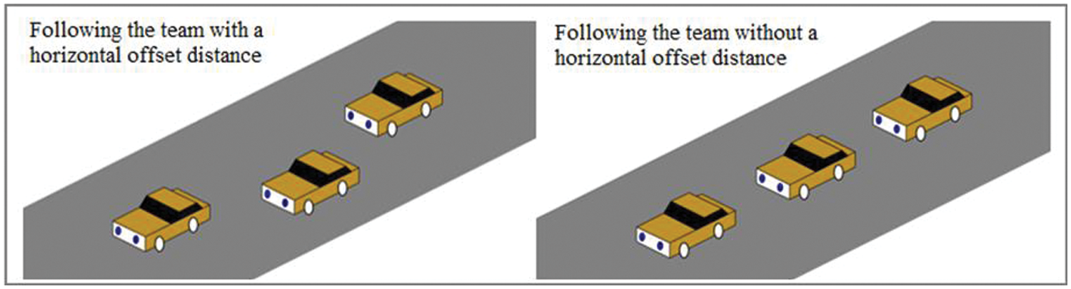
Figure 1: The fleet’s topology

Prior to doing CFD simulations of the fleet, a simulation of a single vehicle is conducted to determine the optimum mesh size and describe the aerodynamic parameters of a single vehicle [15]. The same method is then applied to a study of multiple vehicle queues.

2.1 Geometric Model

Since the 1980s, more than a dozen models with different characteristics have appeared internationally. The most popular among them are the Ahemd, MIRA and DrivAer models. Compared with the Ahemd and DrivAer models, the MIRA model can lower the computational workload and ensure the accuracy of the simulations. The conventional Mira step-back vehicle model [16], one of the typical car aerodynamic physical models, is utilized in this study. Compared with the square-back and fast-back models in the MIRA model, the step-back model wake has three-dimensional separation, return flow, and high turbulence, which are more closely related to the vehicle wake flow characteristics. The length, width and height of the full-size model are 4165, 1625 and 1420 mm, respectively [17]. Fig. 2 depicts the measurements and CAD model of the typical step-back MIRA model.

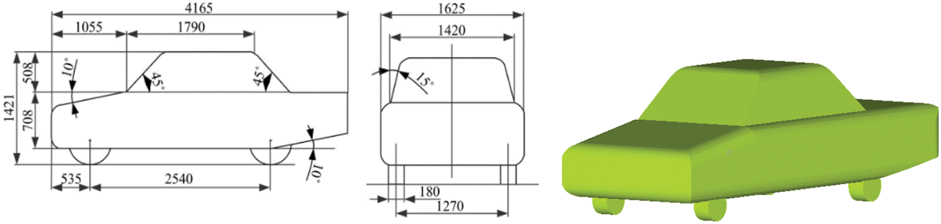
Figure 2: Typical step-back MIRA model (unit: mm)

2.2 Computing Domain Setting and Grid Division

To accurately analyze the characteristics of the vehicle queue flow field, it is essential that the blockage ratio of the virtual wind tunnel be less than 10%, preferably between 3% and 5%. In light of this, the height and width of the virtual wind tunnel were designed to be 3 times and 11 times the height and length of the vehicle, respectively. Meanwhile, in order to ensure the full development of the airflow, the distance between the front of the leading vehicle and the wind tunnel entrance, and the distance between the trailing vehicle’s rear end and the wind tunnel exit are set to 3 times and 7 times the vehicle length, respectively.

In ANSYS ICEM, the vehicle body and rectangular external flow field are meshed, with the vehicle body surface mesh consisting of quadrilateral cells, the wind tunnel surface mesh being of triangular cells, and the body mesh composed of a mixed mesh. A 30 by 70 mm density box is used to guarantee the natural transition of the body mesh between the vehicle and the wind tunnel. In addition, three layers are bonded to the body’s surface near the wall to better collect the surface gas flow. Approximately 2.56 million meshes are generated in the computational simulation area. Fig. 3 depicts the size and mesh model of the external flow field.

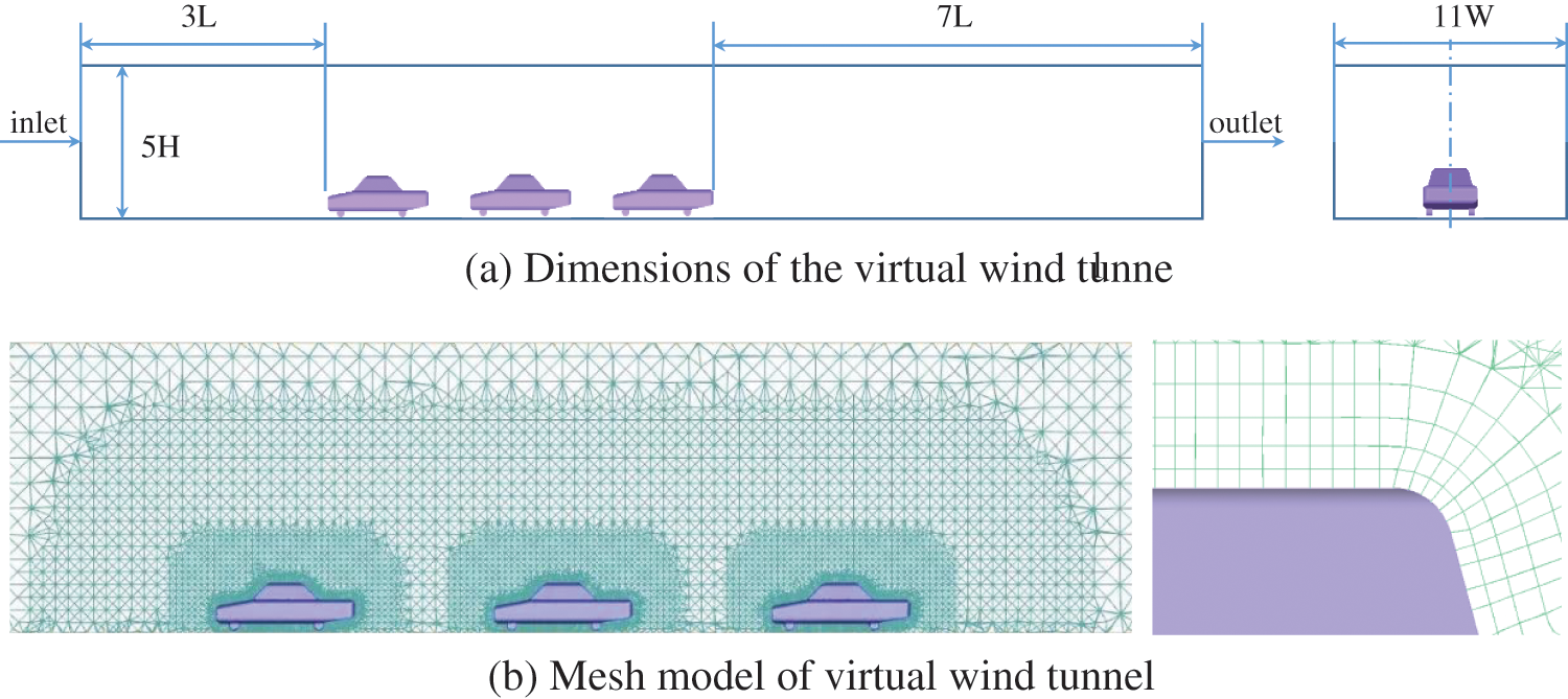
Figure 3: Dimensions and mesh model of virtual wind tunnel

2.3 Boundary Conditions

For the simulation calculation, the standard k-ε turbulence model is employed. The intake and the outlet of the flow field are designated as the velocity inlet and the pressure outlet, respectively. The top surface and left and right sides of the calculation domain are designated as the slip wall. As depicted in Fig. 4, the ground, vehicle body surface, and wheels serve as the nonslip wall. In addition, the pace of the moving slip wall is regulated to match the wind speed.

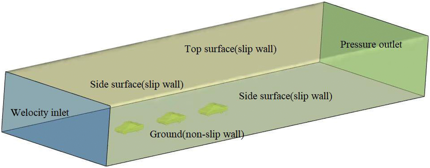
Figure 4: Boundary condition setting

2.4 Mathematical Model

In simulations of fluid dynamics, it is assumed that the fluid obeys the three conservation rules of mass, energy, and momentum in the flow process [18]. The flow outside the vehicle is often considered as incompressible, isothermal, and adiabatic turbulent flow. Since heat transmission is not concerning, the solution equations include only mass conservation and momentum conservation equations, which are stated as follows.

Law of mass conservation:

∂ρ∂t+∂(ρu)∂x+∂(ρv)∂y+∂(ρw)∂z=0 (1)

The conservation of momentum law:

∂(ρu)∂t+div(ρuu)=−∂p∂x+∂τxx∂x+∂τyx∂y+∂τzx∂z (2)

∂(ρv)∂t+div(ρvu)=−∂p∂y+∂τxy∂x+∂τyy∂y+∂τzy∂z (3)

∂(ρw)∂t+div(ρwu)=−∂p∂z+∂τxz∂x+∂τyz∂y+∂τzz∂z (4)

where ρ is the fluid density; t is time; u, v and w are the components of the velocity vector in x, y and z directions, respectively; T is the temperature; p is the pressure on the fluid micro-element; τxx, τyx and τzx are the viscous stress in the x-direction; τxy, τyy and τzy are the viscous stress in the y-direction; τxz, τyz and τzz are the viscous stress in the z-direction.

The steady-state RANS k-ε turbulence model with standard wall functions is employed for CFD simulations in this paper. When the flow is incompressible, the exact formulas can be stated as follows:

k equation:

∂∂t(ρk)+∂∂xi(ρkui)=∂∂xj[(μ+μtσk)∂k∂xj]+Gk−ρε (5)

ε equation:

∂∂t(ρε)+∂xi(ρεui)=∂∂xj[(μ+μtσε)∂k∂xj]+C1εεkGk−C2ερε2k (6)

where Gk is the turbulent kinetic energy generation term; μ is the dynamic viscosity; μt is the turbulent viscosity; C1ε and C2ε are empirical constants taking values of 1.44 and 1.92, respectively; σk and σε are turbulent prandtl values for the k and ε equations, taking values of 1.0 and 1.3, respectively.

The numerical computation method used in this paper is the FVM (Finite Volume Method). The pressure variable is discretized using the second-order scheme, and the momentum, turbulent kinetic energy, and turbulent dissipation rate variables are discretized using the second-order upwind scheme, as in literature [19]. The SIMPLE algorithm is employed to solve the pressure-velocity coupling problem; the same algorithm are used in literature [20,21].

The vehicle fuel saving rate [22] shall be calculated by developing a mathematical model of the vehicle aerodynamics. In this paper, assuming the car is driving at a constant speed on a flat road, the ramp and acceleration resistance can be neglected. According to automobile theory, the calculation derivation process is as follows:

Ft=Ff+Fw=mgf+CdAρva2/2 (7)

where Ft, Ff and Fw are the vehicle driving force, rolling resistance and the air resistance, respectively; m is the quality of the vehicle; g is gravity acceleration; f is the rolling resistance coefficient; Cd is the aerodynamic resistance coefficient; A is the windward area of the vehicle; ρ is the air density, usually taken as 1.2258 kg/m3; va is the driving speed.

The expression for vehicle air resistance can be further rewritten as follows:

Fw=CdAva221.15 (8)

The following is the formula for calculating engine power:

Pe=vaFtηt (9)

where Ft is the vehicle driving force, which can be obtained from the vehicle driving equation; va is the driving speed; ηt is the mechanical efficiency of the transmission system.

The fuel consumption per hundred kilometers of an automobile moving at a steady speed is described as follows:

Qs=Pemf1.02vaρfg (10)

where mf is the fuel consumption; ρf is the fuel density; g is gravity acceleration.

The following two equations define the air drag coefficient decrease rate (Eq. (11)) and the fuel savings rate (Eq. (12)).

ΔCd=Cd0−CdCd0 (11)

ΔQs=Qs0−QsQs0 (12)

where Cd0 and Cd are the single-vehicle drag coefficient and the mean drag coefficient of the queue, respectively; Qs0 and Qs are the 100 km fuel consumption of the single-vehicle and the average 100 km fuel consumption of the fleet, correspondingly.

Eq. (13) defines the relationship between the rate of fuel savings and the rate of drag coefficient reduction. Here μ indicates the factors affecting fuel consumption at a constant speed on a horizontal road.

ΔQs=ΔCd1+μ (13)

3  Results and Analysis

3.1 Simulation Results for Single-Vehicle

Using a virtual wind tunnel simulation, the aerodynamic drag coefficients of a single vehicle were computed and compared with test data from the HD-2 wind tunnel [23], the TJ-2 wind tunnel [24], and the IVK wind tunnel [25], as shown in Fig. 5.

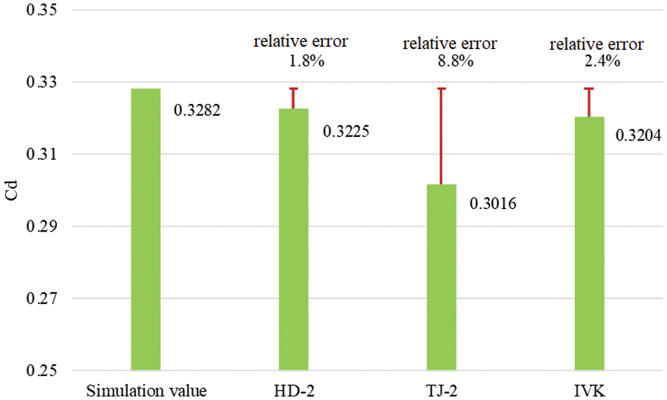
Figure 5: Validation study comparing air resistance coefficients between simulation and wind tunnel experiments

Fig. 5 presents a validation exercise for the numerical simulation using the MIRA model and the same test conditions as the wind tunnel experiments. The aim was to assess the accuracy of the simulation method by comparing the simulated coefficient of air drag (Cd) with the corresponding experimental measurements. The simulation results yielded a coefficient of air drag (Cd) of 0.3282. When comparing these results to the HD-2, TJ-2, and IVK wind tunnel experimental measurements, the relative errors were found to be 1.8%, 8.8%, and 2.4%, respectively. These low relative errors indicate a close agreement between the simulation and experimental results. The high level of agreement between the simulation and experimental data supports the reliability and accuracy of the numerical simulation method employed in this research. This finding has significant implications as it allows for further investigation and exploration of different scenarios in a cost-effective and efficient manner.

The outflow field characteristics of a single vehicle are investigated here for comparison with the simulation findings of a vehicle queue. Figs. 6 and 7 represent the pressure cloud and velocity vector diagrams for a single vehicle, respectively. They illustrate the causes of the generation of differential pressure resistance of the vehicle. From Fig. 6, it can be seen that the vehicle body has the highest windward pressure at the air intake grille, followed by the windshield, which are immediately subjected to the airflow and are the primary cause of the vehicle’s drag. The rear of the vehicle body produces a negative pressure zone due to airflow separation and vortex flow, as shown in the Fig. 7. It is visible that the air flowing to the rear of the vehicle breaks away from the body and forms a vortex flow at the rear of the vehicle, resulting in a negative pressure zone. The pressure difference between this negative pressure and the positive pressure at the front of the car creates a force in the opposite direction of travel, which is the differential pressure resistance.

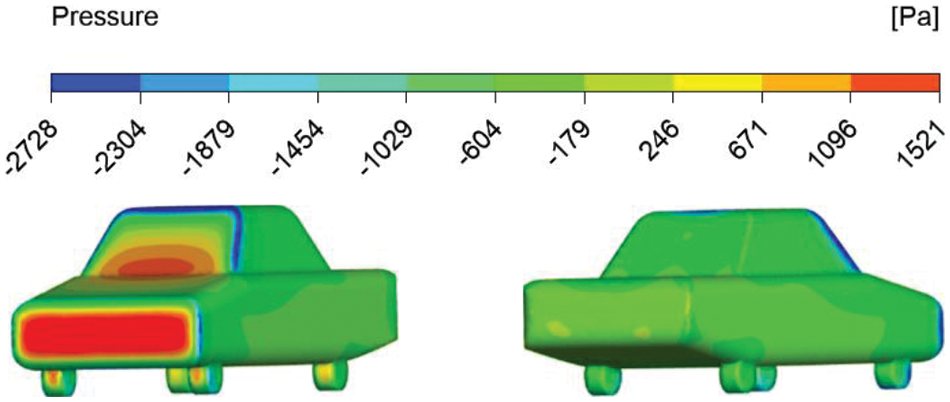
Figure 6: Single-vehicle’s pressure cloud map

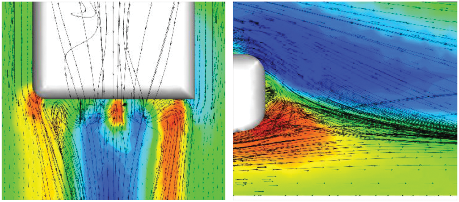
Figure 7: Single-vehicle’s velocity vector chart

3.2 Effect of Longitudinal Spacing and Lateral Offset Distance

The effects of longitudinal vehicle spacing and lateral offset distance on the fleet’s drag coefficient are explored for a three-vehicle queue. The vehicle speed is assumed to be 50 kilometers per hour. The longitudinal inter-vehicle distances are varied in the range of 0.1 to 3L, and the lateral offset distances are 0, 1/6, 1/3, 1/2, and 1W, where L is a vehicle length and W is a vehicle width. Fig. 8 illustrates the fleet’s average air drag coefficients for various longitudinal vehicle and lateral offset distances. It also shows how the inter-vehicle distance and lateral offset distance affect the air drag coefficient of each car in the queue.

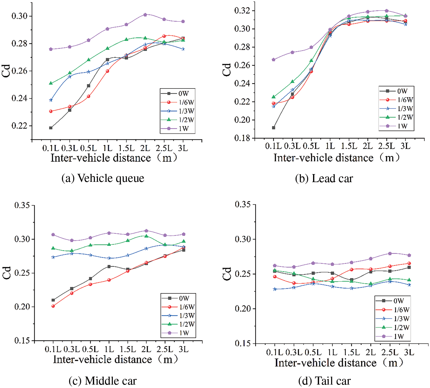
Figure 8: Drag coefficient for the queue and each vehicle in the queue

Fig. 8a reveals that the average coefficient of drag while cars travel in formation is lower than the coefficient of drag for a single car due to the queue fleet, as presented by Gao et al. [26]. The fleet average air drag coefficient achieves a maximum value of 0.296 when the inter-vehicle distance is 2L and the lateral offset distance is 1W. The shielding effect of the front car on the rear car decreases gradually as longitudinal spacing increases, and the fleet’s drag coefficient increases gradually under the fixed lateral offset distance. And when the longitudinal distance exceeds 2L, its effect on the fleet drag coefficient is minimal. When the longitudinal distance is a fixed value, the fleet drag coefficient increases with the lateral offset distance, and the change in queue air drag coefficient is especially pronounced between 0 and 1.5L.

Figs. 8b∼8d illustrate the trend of variation in drag coefficient for each car in the cohort. From Fig. 8b, it can be seen that the air drag coefficient of the leading car changes a lot between 0 and 1.5L, as well as that the coefficient gradually goes up as the lateral offset distance goes up. After the inter-vehicle distance surpasses 1.5L, the resistance coefficient of the leading car remains steady and the lateral offset distance has little effect on it. Fig. 8c shows that the air resistance coefficient of the middle car gradually increases with the increase of the distance between vehicles under the condition of small lateral offset distance. When the lateral offset distance exceeds 1/3W, the drag coefficient of the middle car is less affected by the longitudinal distance, but is significantly affected by the change of the lateral offset distance, which increases continuously with the growth of the lateral offset distance. According to Fig. 8d, the change in longitudinal spacing has a negligible influence on the resistance coefficient of the rear car, however the change in lateral offset distance has a significant effect.

Figs. 9 and 10 depict the vehicle pressure clouds and velocity vector plots for various lateral offset distances at a constant inter-vehicle distance, respectively. As shown in Fig. 9, When compared to the leading vehicle, all other vehicles show a noticeable decrease in pressure, which is consistent with the results reported by He et al. [27]. As the lateral offset distance rises, the head pressure of the middle car progressively increases, which was also reported by Mokhtar et al. [28]. The head pressure of the tail car is somewhat less than that of the lead car and the middle car, and the position of the high-pressure area of the tail car’s head pressure fluctuates continuously. In conjunction with the velocity vector plots in Fig. 10, it is evident that when the lateral offset distance gradually increases, the shielding effect of the lead car on the middle car gradually reduces, hence increasing the middle car’s head pressure. The results show that the tail car will be affected by the middle and the head car at the same time, resulting in a change in the location of its head’s high-pressure area.

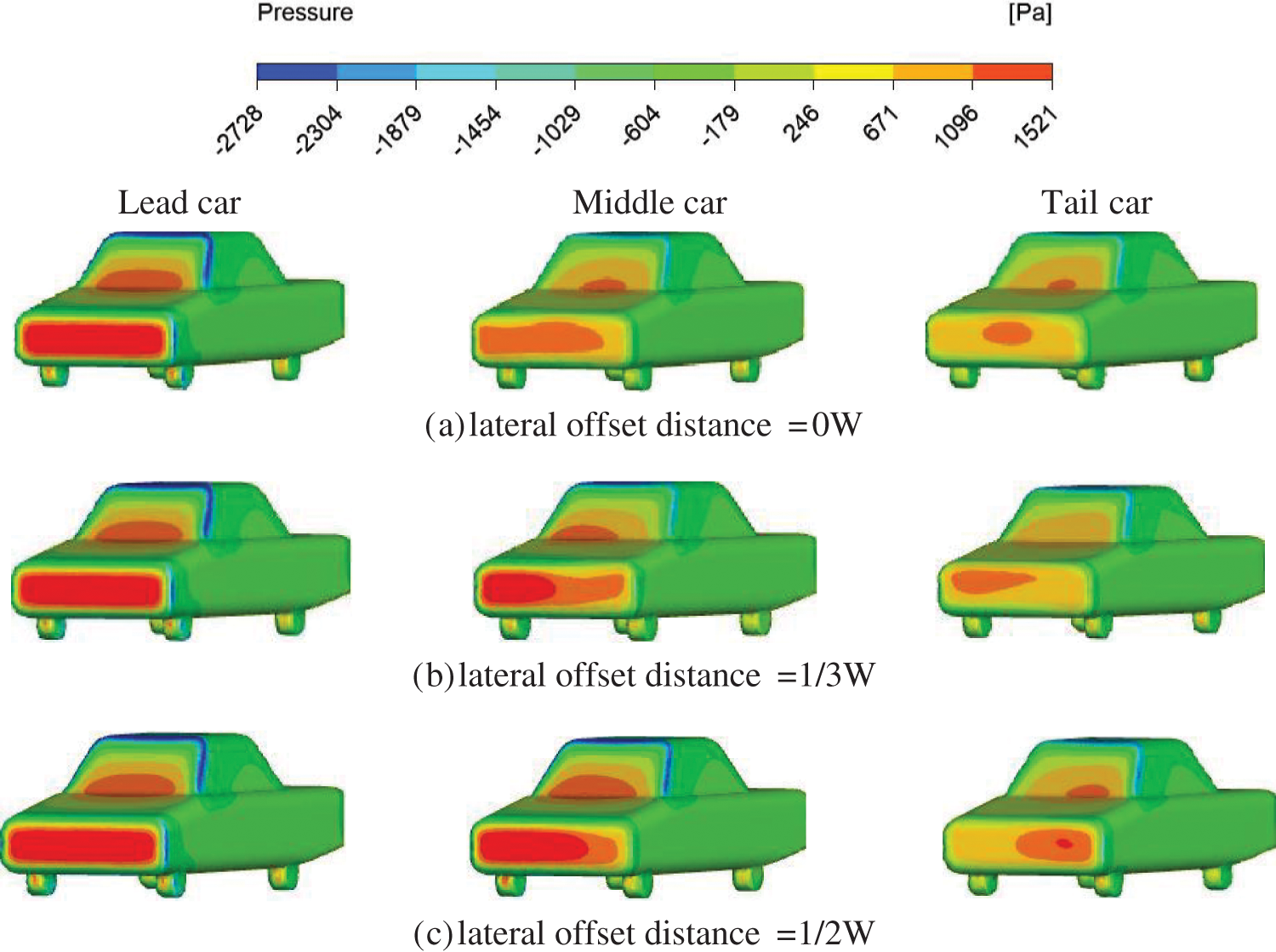
Figure 9: Vehicle pressure cloud maps at a constant inter-vehicle distance

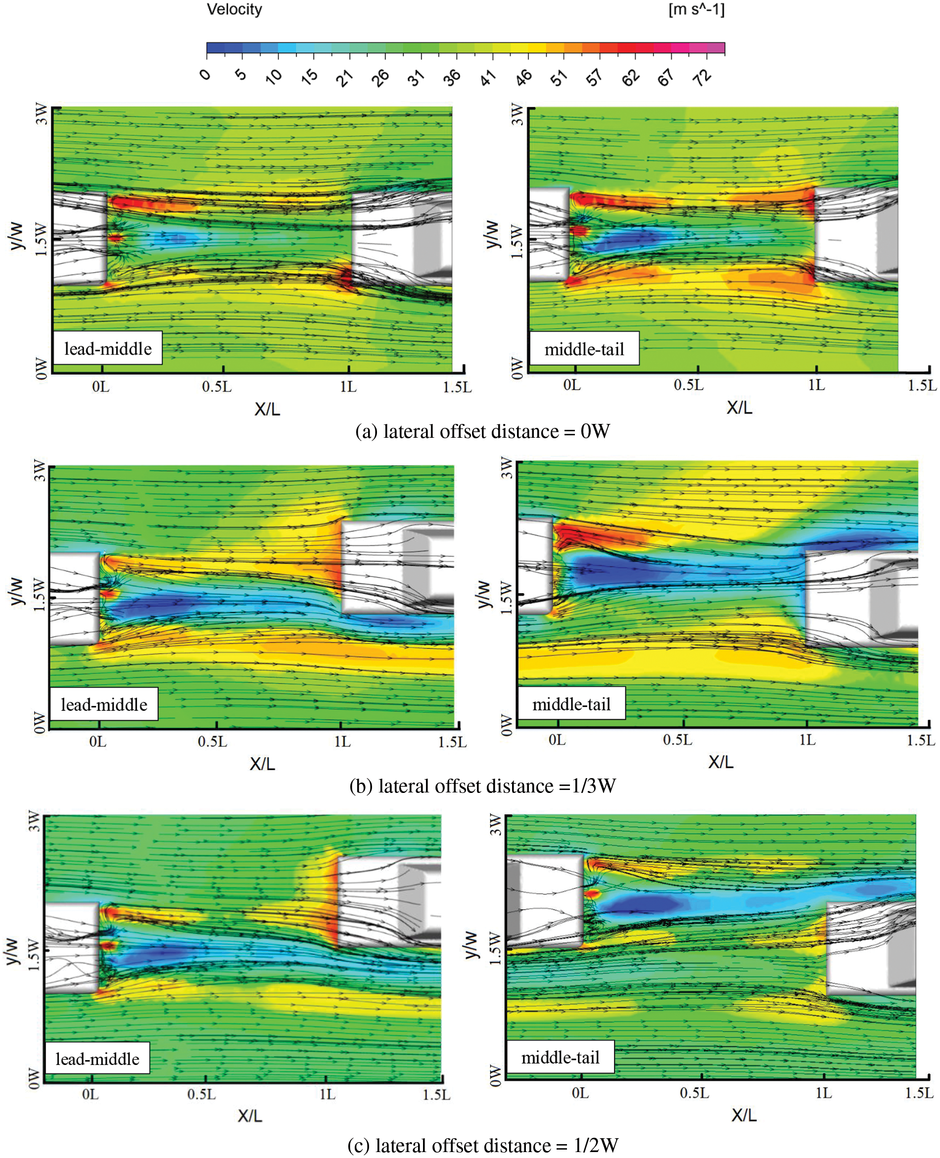
Figure 10: Vehicle velocity vector plots at a constant inter-vehicle distance

Fig. 11 illustrates the fuel-saving rates of the vehicle queue and each vehicle in the fleet at various longitudinal and lateral offset distances. As shown in Fig. 11a, the fuel-saving rate of the vehicle queue drops steadily with the rising of the inter-vehicle distance and lateral offset distance. Under the current configuration parameters, the fleet average fuel saving rate can reach up to 3.63%. From Fig. 11b, it can be learned that when the distance between vehicles varies from 0 to 1.5L, the fuel saving rate of the lead vehicle decreases significantly with the increase of the distance between vehicles. When the lateral offset distance is ranged from 0 to 1/6W, the middle car’s fuel saving rate increases with the lateral offset distance until it reaches its maximum at 1/6W, after which it decreases with the lateral offset distance, as shown in Fig. 11c. According to Fig. 11d, the tail vehicle’s fuel savings vary with the lateral offset distance. The fuel-saving impact is evident for lateral offset distances ranging from 0 to 1/3W, which is primarily due to the combined influence of airflow from the lead and middle cars on the rear car.

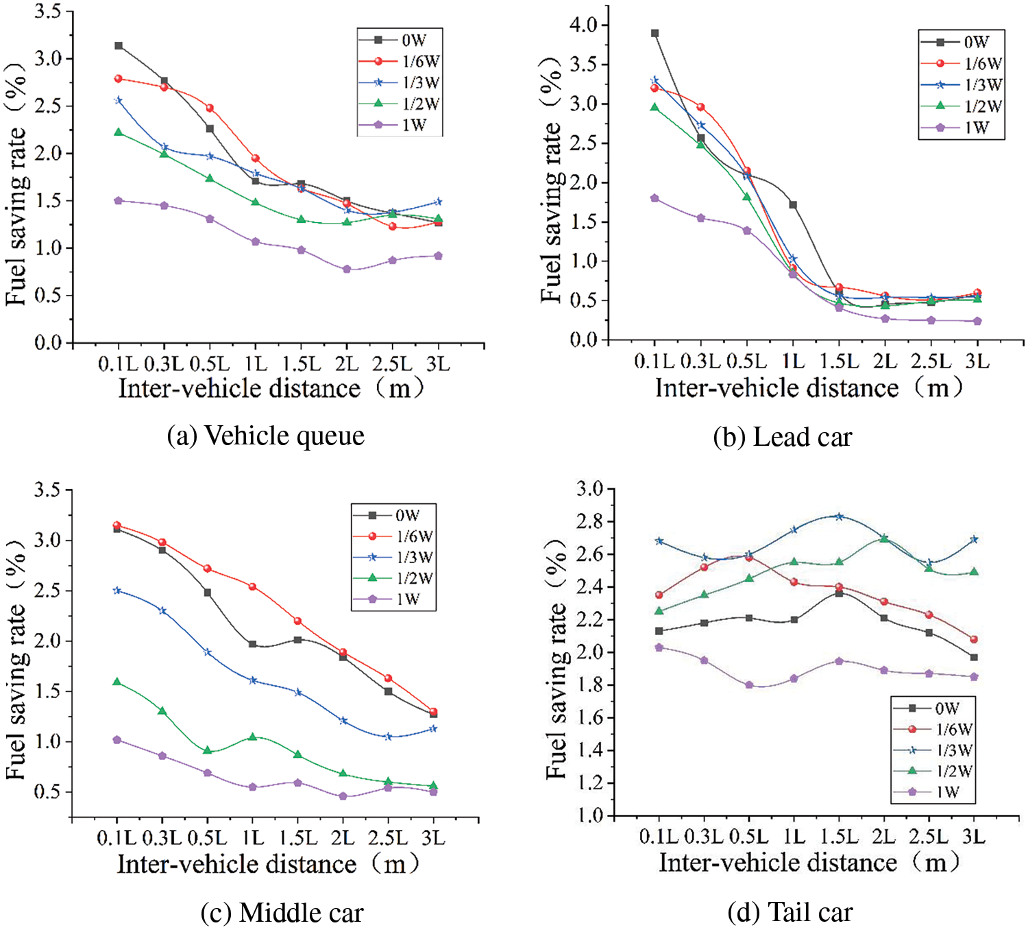
Figure 11: Fuel saving rate for the queue and each vehicle in the queue

3.3 Effect of Vehicle Velocity and Lateral Offset Distance

The change of resistance coefficient of three-car queue with vehicle speed and lateral offset distance is investigated when the longitudinal inter-vehicle distance is held constant (1L in this article). It is assumed that the variation range of vehicle speed is from 50 to 90 km/h, and the lateral offset distance is from 0 to 1W. In this study, the simulation findings for vehicle speeds of 60 km/h and lateral offset distances of 0, 1/6, and 1/2W serve as examples. The resistance coefficient of the vehicle queue decreases as the lateral offset distance changed between 0 and 1/6W. However, when the lateral offset exceeds 1/6W, the drag coefficient increases.

Fig. 12 depicts the variation of air resistance coefficients of the fleet and each vehicle in queue at various speeds and lateral offset distances. The vehicle queue’s average resistance coefficient is substantially lower than that of a single car (0.3282), as displayed in Fig. 12a. The queue’s resistance coefficient increases from 50 to 60 km/h when the lateral offset distance remains constant. After 60 km/h, the effect of speed on the queue’s air drag coefficient becomes negligible. At constant speed, the vehicle queue’s coefficient decreases when the lateral offset distance is ranging from 0 and 1/6W and rises when it exceeds 1/6W. When the vehicle speed is 50 km/h and the lateral offset distance is 1/6W, the fleet average aerodynamic drag coefficient achieves a minimum value of 0.262. According to Figs. 12b and 12c, when the lateral offset distance is changed from 0 to 1W, the front and middle cars’ resistance coefficients decrease and then increase, with the minimum value being attained at 1/6W. The drag coefficients of the lead and the middle cars rise with the increase of speed. Fig. 12d demonstrates that the variation in the air resistance coefficient of the tail car is more complex. When the lateral offset distance varies from 0 to 1W, the air drag coefficient of the tail car first increases, then reduces, and then raises once again. This is mainly because the tail car is most affected by the wakes of both the middle and front cars.

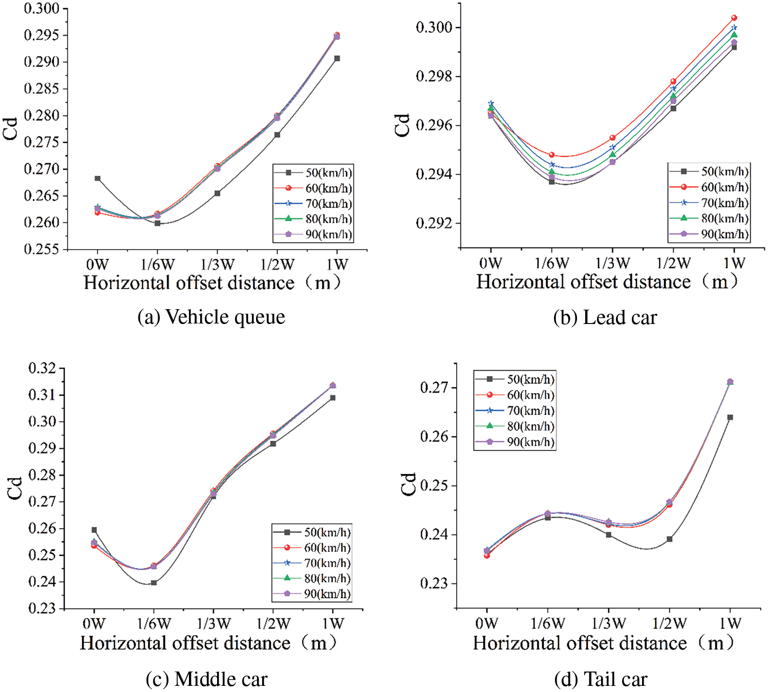
Figure 12: Drag coefficient for the queue and each vehicle in the queue

Figs. 13 and 14 depict the pressure and velocity distribution of each car in a three-car queue at varying lateral offset distances for a fixed car speed. Combining Figs. 13 and 14, it is clear that the lead car’s head pressure distribution does not change significantly with lateral offset distance, as concluded by Törnell et al. [29]; the middle car’s head impact area is constantly changing, resulting in more noticeable changes in the pressure distribution; and when the lateral offset distance reaches 1/2W, the middle car’s head pressure distribution is comparable to that of the lead car. The pressure on the head of the tail car is lower when compared to the head and middle cars; however, as the lateral offset distance increases, the pressure on the head of the tail car gradually increases. The location of the tail car’s high-pressure area is constantly shifting due to the combined action of the head and middle cars’ wake.

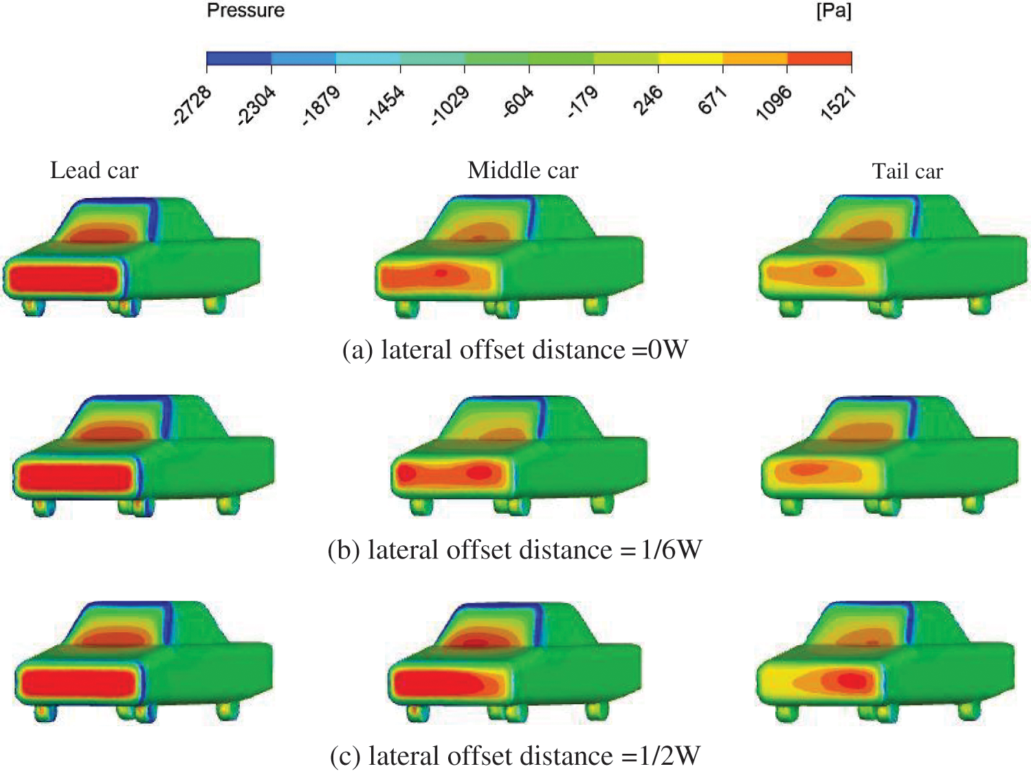
Figure 13: Vehicle pressure cloud maps at a constant vehicle velocity

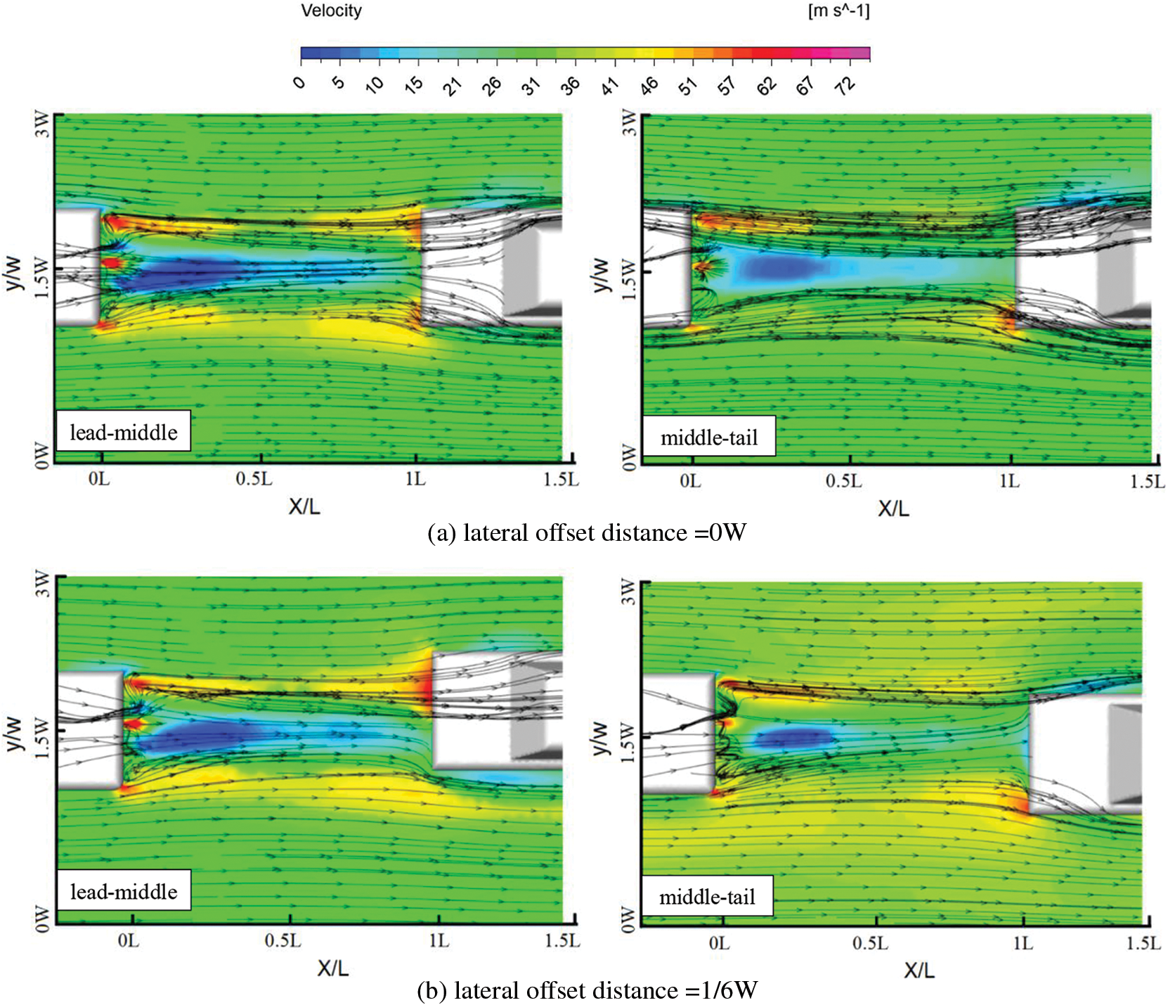
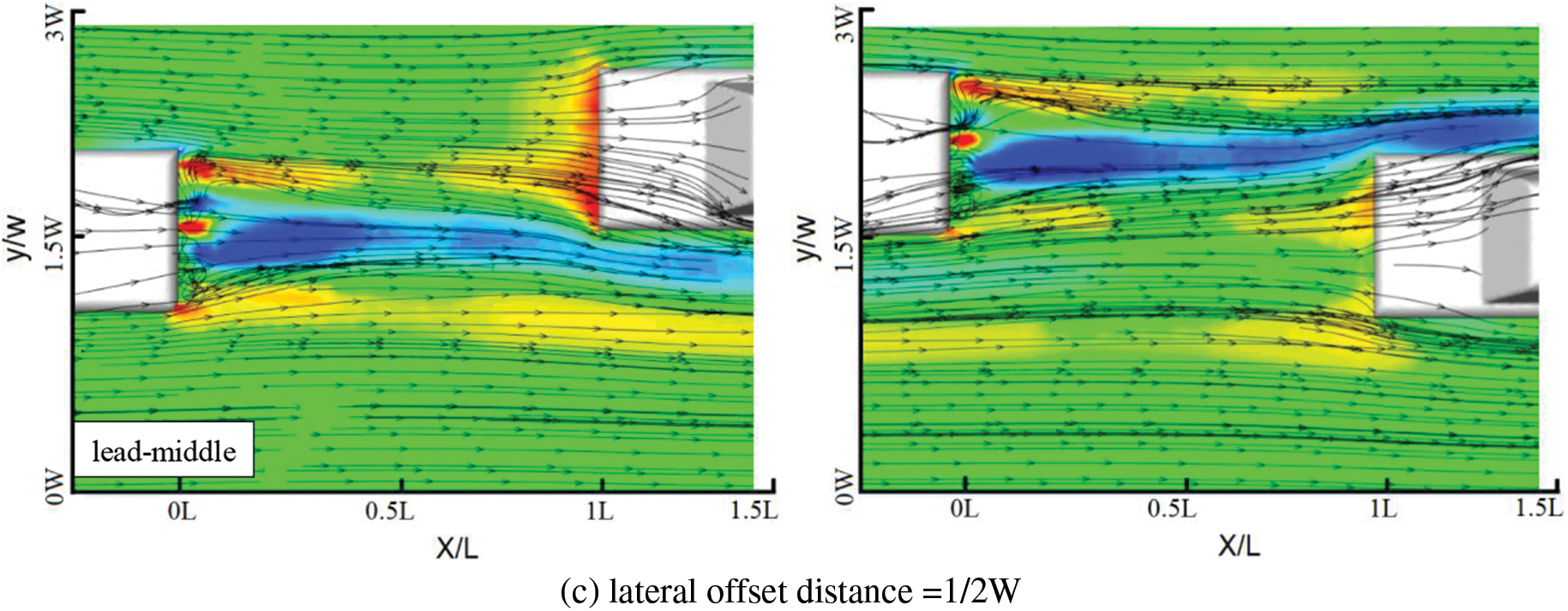
Figure 14: Vehicle velocity vector plots at a constant vehicle velocity

Fig. 15 illustrates the impacts of vehicle speed and lateral offset distance on the fleet’s and individual vehicle’s fuel savings rate, from which the following can be deduced. When the lateral offset distance is fixed, the vehicle queue’s fuel-saving rate rises progressively with increasing speed. Under the same speed, the fleet’s fuel-saving rate decreases as the lateral offset distance increases. The rate of fuel savings for the leading, middle, and trailing vehicles changed correspondingly. Under identical conditions of speed and lateral offset distance, the fuel efficiency of each vehicle varies.

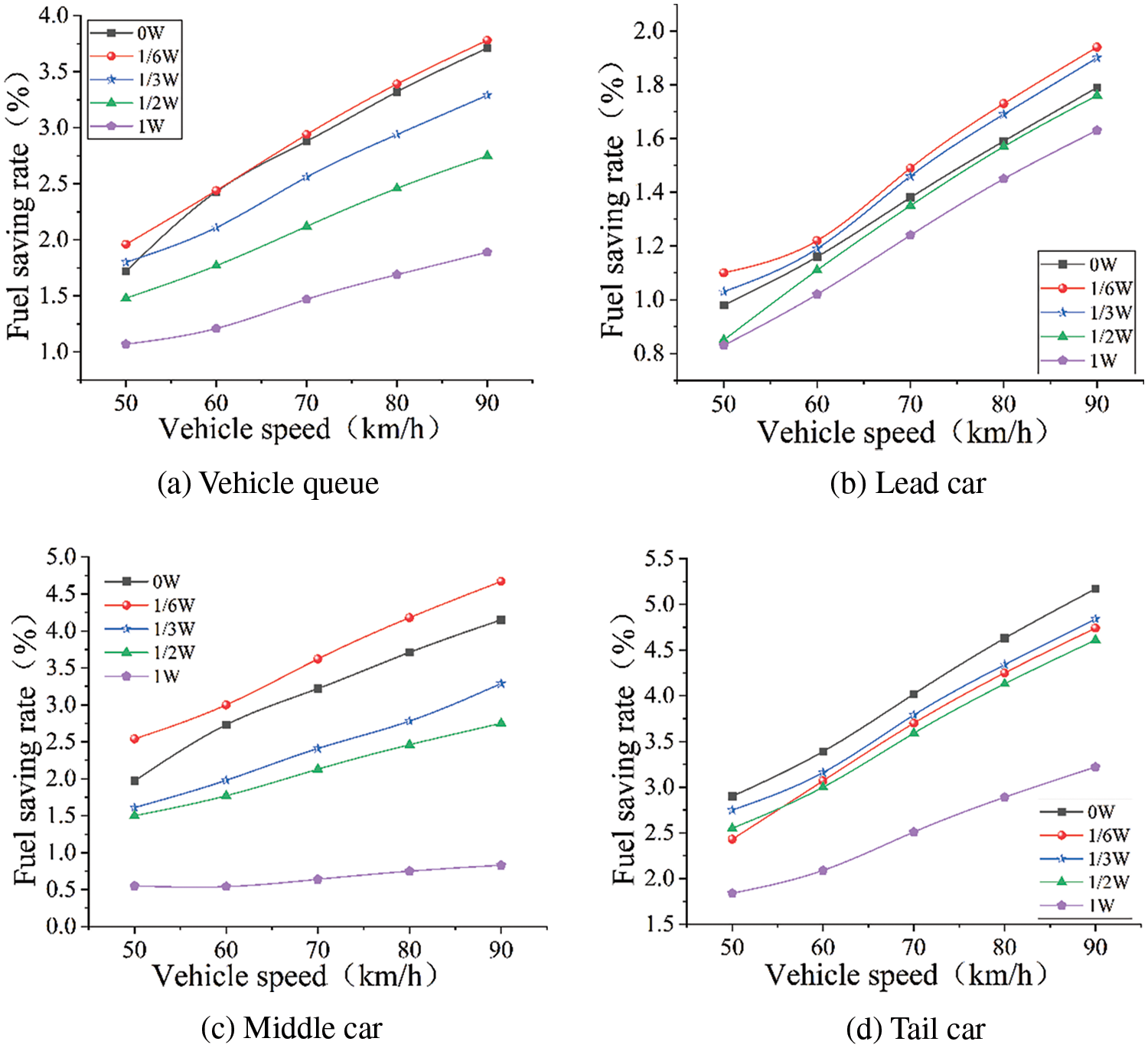
Figure 15: Fuel saving rate for the queue and each vehicle in the queue

4  Conclusions

Vehicle queues have been the subject of much aerodynamic research, which has yielded numerous findings. This article examines the aerodynamic qualities and fuel efficiency of a three-vehicle formation using the conventional Mira model with varying inter-vehicle distances, vehicle speeds, and lateral offset distances, and draws the following conclusions:

(1) The fleet has a lower average air drag coefficient than a single vehicle.

(2) Under the same speed class, as inter-vehicle distance and lateral offset distance rise, the average air drag coefficient of the fleet grows while the rate of fuel savings changes in the opposite direction.

(3) Under the same inter-vehicle spacing, assuming the vehicle speed remains constant, the average air drag coefficient of the fleet drops and subsequently increases as the lateral offset distance grows, with a minimum value of 1/6W. The change of the fuel-saving rate is inversely proportional to the coefficient of air drag, and the fuel-saving rate increases with increasing speed for varying lateral offset distances.

This work studied vehicle formation’s aerodynamic features and fuel efficiency under the different configuration parameters. The results of the study showed that the aerodynamic advantage of the vehicle queue can be better utilized when the inter-vehicle distance is less than 2L and the lateral offset distance is less than 1/6W. The conclusion provides a theoretical foundation for constructing a vehicle formation driving strategy. In the article, the vehicle speed is constant. But in reality, a vehicle’s working conditions change constantly during the driving process, which causes the speed also to change. Therefore, the research on the vehicle fleet under variable speed conditions will be studied in the future.

Acknowledgement: None.

Funding Statement: This study was financially supported by the National Natural Science Foundation of China (52072156) and the Postdoctoral Foundation of China (2020M682269).

Author Contributions: Study conception and design: Lili Lei; Data collection: Ze Li, Jing Wang; Analysis and interpretation of results: Ze Li, Haichao Zhou; Draft manuscript preparation: Jing Wang, Wei Lin. All authors reviewed the results and approved the final version of the manuscript.

Availability of Data and Materials: All data generated or analyzed during this study are included in this published article.

Conflicts of Interest: The authors declare that they have no conflicts of interest to report regarding the present study.

References

1. Dong, J., Gao, Q., Li, J., Li, J., Hu, Z. et al. (2023). Innovative modeling strategy of wind resistance for platoon vehicles based on real-time disturbance observation and parameter identification. Proceedings of the Institution of Mechanical Engineers, Part D: Journal of Automobile Engineering. https://doi.org/10.1177/09544070231153213 [Google Scholar] [CrossRef]

2. Gungor, O. E., She, R., Al-Qadi, I. L., Ouyang, Y. (2020). One for all: Decentralized optimization of lateral position of autonomous trucks in a platoon to improve roadway infrastructure sustainability. Transportation Research Part C: Emerging Technologies, 120, 102783. https://doi.org/10.1016/j.trc.2020.102783 [Google Scholar] [CrossRef]

3. Ebrahim, H., Dominy, R. (2020). Wake and surface pressure analysis of vehicles in platoon. Journal of Wind Engineering and Industrial Aerodynamics, 201, 104144. https://doi.org/10.1016/j.jweia.2020.104144 [Google Scholar] [CrossRef]

4. Yang, Z. F., Li, S. H., Liu, A. M., Yu, Z., Zeng, H. J. (2019). Simulation study on energy saving of passenger car platoons based on DrivAer model. Energy Sources, Part A: Recovery, Utilization, and Environmental Effects, 41(24), 3076–3084. [Google Scholar]

5. Abdul-Rahman, H., Moria, H., Rasani, M. R. (2021). Aerodynamic study of three cars in tandem using computational fluid dynamics. Journal of Mechanical Engineering and Sciences, 15(3), 8228–8240. [Google Scholar]

6. Ebrahim, H., Dominy, R., Martin, N. (2021). Aerodynamics of electric cars in platoon SAGE publications. Journal of Automobile Engineering, 235(5), 1396–1408. [Google Scholar]

7. Tbmell1, J., Sebben, S., Sderblom, D. (2021). Influence of inter-vehicle distance on the aerodynamics of a two-truck platoon. International Journal of Automotive Technology, 22(3), 747–760. [Google Scholar]

8. Kaluva, S. T., Pathak, A., Ongel, A. (2020). Aerodynamic drag analysis of autonomous electric vehicle platoons. Energies, 13(15), 4028. https://doi.org/10.3390/en13154028 [Google Scholar] [CrossRef]

9. Siemon, M., Smith, P., Nichols, D., Bevly, D., Heim, S. (2018). An integrated CFD and truck simulation for 4 vehicle platoons. SAE Technical Paper, 2018-01-0797. https://doi.org/10.4271/2018-01-0797 [Google Scholar] [CrossRef]

10. Good, G. L., Resnick, M., Boardman, P., Clough, B. (2021). An investigation of aerodynamic effects of body morphing for passenger cars in close-proximity. Fluids, 6(2), 64. https://doi.org/10.3390/fluids6020064 [Google Scholar] [CrossRef]

11. Cerutti, J. J., Cafiero, G., Iuso, G. (2021). Aerodynamic drag reduction by means of platooning configurations of light commercial vehicles: A flow field analysis. International Journal of Heat and Fluid Flow, 90, 108823. https://doi.org/10.1016/j.ijheatfluidflow.2021.108823 [Google Scholar] [CrossRef]

12. Ebrahim, H., Dominy, R. (2021). The effect of afterbody geometry on passenger vehicles in platoon. Energies, 14(22), 7553. https://doi.org/10.3390/en14227553 [Google Scholar] [CrossRef]

13. Robertson, F. H., Soper, D., Baker, C. (2021). Unsteady aerodynamic forces on long lorry platoons. Journal of Wind Engineering & Industrial Aerodynamics, 209, 104481. https://doi.org/10.1016/j.jweia.2020.104481 [Google Scholar] [CrossRef]

14. Hussein, A., Rakha, H. (2021). Vehicle platooning impact on drag coefficients and energy/fuel saving implications. IEEE Transactions on Vehicular Technology, 71(2), 1199–1208. [Google Scholar]

15. Sun, D. J., Shi, X., Zhang, Y., Zhang, L. (2021). Spatiotemporal distribution of traffic emission based on wind tunnel experiment and computational fluid dynamics (CFD) simulation. Journal of Cleaner Production, 282, 124495. https://doi.org/10.1016/j.jclepro.2020.124495 [Google Scholar] [CrossRef]

16. Du, Q. Q., Hu, X. J., Li, Q. F., Yang, B. (2013). Numerical optimization research on rear characteristic angles based on MIRA model for aerodynamic drag reduction. Advanced Materials Research, 774–776, 428–432. [Google Scholar]

17. Zhou, H., Chen, G., Yang, Z. G., Zhu, H. (2018). Validation experiments for LBM simulations of MIRA model. Academic Annual Conference of Automotive Aerodynamic Committee 2018 Shanghai, China. [Google Scholar]

18. Song, M. T., Chen, F., Ma, X. X. (2021). Organization of autonomous truck platoon considering energy saving and pavement fatigue. Transportation Research Part D, 90, 102667. https://doi.org/10.1016/j.trd.2020.102667 [Google Scholar] [CrossRef]

19. Gan, E. C. J., Fong, M., Ng, Y. L. (2021). CFD analysis of slipstreaming and side drafting techniques concerning aerodynamic drag in NASCAR racing. CFD Letters, 12(7), 1–16. [Google Scholar]

20. Zhang, X. T., Robertson, F. H., Soper, D., Hemida, H., Huang, S. D. (2021). Investigation of the aerodynamic phenomena associated with a long lorry platoon running through a tunnel. Journal of Wind Engineering and Industrial Aerodynamics, 210, 104514. https://doi.org/10.1016/j.jweia.2020.104514 [Google Scholar] [CrossRef]

21. Farid, T., Shakeel, A., Sajid, M. (2019). An evaluation of open source CFD for study of aerodynamics of vehicle platooning. Proceedings of the ASME-JSME-KSME 2019 8th Joint Fluids Engineering Conference, Vol. 2: Computational Fluid Dynamics, V002T02A068.San Francisco, California, USA, ASME. https://doi.org/10.1115/AJKFluids2019-5130 [Google Scholar] [CrossRef]

22. Zhang, L., Chen, F., Ma, X. X., Pan, X. D. (2020). Fuel economy in truck platooning: A literature overview and directions for future research. Journal of Advanced Transportation, 2020, 1–10. [Google Scholar]

23. Qi, G. Z., Shi, W., Jian, C., Lin, Q. Z. (2011). Wind tunnel test research on MIRA model group tail shape. Science and Technology Guide, 29(8), 67–71. [Google Scholar]

24. Quintino, L. K., Gutierrez, J. C., Cancino, L. R. (2022). Aerodynamic investigation of a MIRA fastback modle geometry using CFD techniques based on experimental wind tunnel analysis. 19th Brazilian Congress of Thermal Sciences and Engineering,Bento Gonçalves, RS, Brazi. [Google Scholar]

25. Xian, Q., Feng, Y., Long, J. Z. (2021). Simulation analysis of the influence of the rear structure of step back vehicle on the aerodynamic characteristics of the rear flow field. Journal of Automobile Safety and Energy Conservation, 12(3), 314–321. [Google Scholar]

26. Gao, W., Deng, Z., Feng, Y., He, Y. (2020). Numerical simulation and analysis of aerodynamic characteristics of road vehicles in platoon. Proceedings of the Canadian Society for Mechanical Engineering International Congress 2020,Charlottetown, PE, Canada. [Google Scholar]

27. He, M., Huo, S., Hemida, H., Frederick, B., Francis, H. et al. (2019). Detached eddy simulation of a closely running lorry platoon. Journal of Wind Engineering and Industrial Aerodynamics, 193, 103956. https://doi.org/10.1016/j.jweia.2019.103956 [Google Scholar] [CrossRef]

28. Mokhtar, W., Dinger, K., Kachare, S., Hossain, M., Britcher, C. (2020). A CFD study investigating drag reduction for different offset and inline distance for two trucks platooning. Journal of Energy and Power Engineering, 14, 143–150. [Google Scholar]

29. Törnell, J., Sebben, S., Elofsson, P. (2021). Experimental investigation of a two-truck platoon considering inter-vehicle distance, lateral offset and yaw. Journal of Wind Engineering and Industrial Aerodynamics, 213, 104596. https://doi.org/10.1016/j.jweia.2021.104596 [Google Scholar] [CrossRef]