Finite Element Method Simulation of Wellbore Stability under Different Operating and Geomechanical Conditions

1  Introduction

At present, well-completion methods mainly include bare-hole completion and shot-hole completion. The bare-hole completion method suits carbonate or sandstone reservoirs without sand production, which are hard and dense. The shot-hole completion method is suitable for sandstone and fractured carbonate reservoirs, which must be sand-free. Therefore, it is necessary to choose the completion method based on the wellbore stability for different types of reservoirs.

For unstable formations, the completion method with a propped arrangement will be adopted to avoid wellbore collapse during the production process. There are three aspects must be considered as the wellbore stability estimation, including rock mechanics parameters, in-situ stress field, and wellbore stability mechanics. Combining the three aspects, the wellbore stability evaluation model can obtain a rational drilling fluid density range to manage wellbore stability. Westergard [1] studied the stress distribution in a deep well wellbore and applied it to the geological engineering analysis of the wellbore. Braun [2] presented three factors influencing effective ground stress associated with wellbore stability and suggested suitable methods for its solution. Yew et al. [3] proposed a model to calculate the hydration stress distribution around the wellbore from the experimental results of mud shale formations. Yu et al. [4] proposed a model that combines chemical and mechanical effects after considering the fluxes of water and ions into and out of the shale. Gomar et al. [5] used a thermal poroelastic model fully coupled with conduction and convective transport processes to analyze wellbore stability and wellbore rupture. Furthermore, Gomar et al. [6] considered the effect of the thermal conductivity of solid particles and used a thermal wellbore mechanical model fully coupled with conduction and convection transport processes. Thereby, they achieved a transient fully coupled thermal pore elastic finite element analysis of the wellbore stability. Ding et al. [7] developed a new model for determining the pressure threshold for safe drilling, considering the upper limit of the shear damage criterion. Lu et al. [8] developed a mechanical model of wellbore stability for weak plane formation under multi-hole flow, considering the effect of multi-hole flow on the weak plane model. Ding et al. [9] considered the anisotropic permeability effects in laminated shale laminae planes and proposed a new wellbore stability model. Jin et al. [10] established a mechanical model of large displacement wellbore stability by regularly analyzing the stress distribution around a large displacement well. Zou et al. [11] established a stable plane strain mechanical model for gas drilling wellbores by considering the damage characteristics around the wellbore under uniformly distributed loads and unevenly distributed loads. Tang et al. [12] studied wellbore stability during completion tests and production by analyzing reservoir rock mineral fraction, microscopic pore structure, and rock mechanical parameters. Ding et al. [13] developed a mechanical-chemical coupling model for wellbore stability based on the results of shale hydration analysis and shale damage criterion. Liang et al. [14] developed a coupled seepage-mechanization wellbore stability model considering hard and brittle mud shale with a weak face structure and having hydration properties. Zhu et al. [15] developed a coupled flow solid-chemical model for mud shale wellbore stability by considering the wellbore destabilization under mud shale hydration conditions. Wang et al. [16] developed a finite element hydraulic coupling model for borehole instability by considering the introduction of a disturbance damage factor into the classical Mohr–Coulomb yielding criterion. Gao et al. [17] developed a porothermoelastic model by considering the effect of dynamic temperature-perturbation boundary effects on the stability of fractured porous rock. Wei et al. [18] proposed a coupled geomechanical and fluid flow model by considering the anisotropic drilling fluid intrusion within a natural fracture. Mao et al. [19] proposed a method for calculating collapse pressure considering the effect of formation hydration and thus assessing borehole stability. Li et al. [20] used methods such as experimental and numerical simulations and considered the temperature variation of the surrounding rock. Thus, the characteristic law of borehole deformation in deep coalbed methane wells was studied.

From the above studies, it is clear that the current research on wellbore stability mainly about mechanical and chemical aspects, and there is a lack of research on the effect of the production process on wellbore stability. To this end, this paper establishes a finite element model based on the theory of poroelasticity and considers the influence of different working conditions and geomechanical conditions. The Mohr–Coulomb rock damage criterion is then used to determine the rock damage state. From this, the factor of wellbore instability and wellbore stability are calculated to determine whether the wellbore is stable. Finally, a simulation study is carried out with field data to provide a model basis for studying wellbore stability during production.

2  Wellbore Mechanics and Judgment Criteria

There are three aspects of wellhole stability mechanics research; the surrounding rock mechanical characteristics is basis, the ground stress is fundamental cause, and the wellbore stability mechanics model effectively solves wellbore stability [21].

2.1 Mathematical Model of Wellbore Stress

The formation rocks are stable through the interaction of overburden pressure, horizontal in-situ stress, and pore pressure. After the wellbore is drilled, the mechanical equilibrium state transforms to an unsteady state, which leads to the redistribution of stresses on the wellbore envelope [22]. Then, the stress on the rocks surrounding the wellbore will be influenced by the original ground stress, formation pore pressure, well column pressure, rock characteristics, and the geometric shape of the wellbore.

2.1.1 Mathematical Model for Wellbore Stress

As shown in Fig. 1, in the wellbore coordinate system (σr‚σθ‚σz) , the stress redistribution generated with the principal stresses can be represented by six stress components: radial σr , circumferential σθ , axial σz , and shear stress τθz‚τrθ‚τrz .

Figure 1: Wellbore coordinate conversion relationship

In a homogeneous, isotropic and linearly elastic formation, the redistributed wellbore envelope stress expression is obtained by using the Fairhurst slant well equation [23]:

{σr=(σx∞+σy∞2)(1−rw2r2)+(σx∞−σy∞2)(1+3rw4r4−4rw2r2)Cos2θ+τxy∞(1+3rw4r4−4rw4r2)Sin2θ+Pwfrw2r2σθ=(σx∞+σy∞2)(1+rw2r2)−(σx∞−σy∞2)(1+3rw4r4)Cos2θ−τxy∞(1+3rw4r4)Sin2θ−Pwfrw2r2σz=σzz∞−2μ(σx∞−σy∞)rw2r2Cos2θ−4μτxy∞rw2r2Sin2θτrθ=−(σx∞−σy∞2)(1−3rw4r4+2rw2r2)Sin2θ+τxy∞(1−3rw4r4+2rw2r2)Cos2θτθz=(−τxz∞Sinθ+τyz∞Cosθ)(1+rw2r2)τrz=(τxz∞Cosθ+τyz∞Sinθ)(1−rw2r2) (1)

The stress component at the wellbore ( r equal to rw ) can be expressed as:

{σr=Pwfσθ=(σx∞+σy∞)−2(σx∞−σy∞)Cos2θ−4τxySin2θ−PwfσZ=σzz−μ[2(σx∞−σy∞)Cos2θ+4τxySin2θ]τθz=2τyzSin2θ−2τxzSin2θτrθ=0τrz=0 (2)

where Pwf is the column pressure; θ is the well circumference angle; σx∞‚σy∞‚σz∞ is the far-field stress in the x‚y‚z-direction in the local coordinate system of the wellbore; σr is the radial stress; σθ is the circumferential stress; σz is the axial stress; rw is the radius of the wellbore; r is the distance from the centerline of the wellbore; τrθ‚τθz‚τrz is the shear stress parallel to the rθ‚θz‚rz plane; τxz∞‚τyz∞‚τxy∞ is the -far field shear stress parallel to the x−z‚y−z‚x−y plane.

2.1.2 Mathematical Model of Vertical Well Wellbore Stress

In the vertical well scenario, the polar axis direction is the same as the maximum principal stress direction (i.e., σx∞=σH σy∞=σh σzz=σv τxz=τyz=τxy=0 ). So, we can rewrite function (1) as follows:

{σr=Pwfσθ=(σH+σh)−2(σH−σh)Cos2θ−PwfσZ=σV−2μ(σH−σh)Cos2θτrθ=0τθz=0τrz=0 (3)

where σH is the maximum horizontal principal stress; σθ is the minimum horizontal principal stress; σz is the vertical stress.

2.1.3 Mathematical Model of Wellbore Effective Stress

In porous media, the formation pore medium around the wellbore, as shown in Fig. 2, is subjected to far-field stress, in-well pressure, and pore fluid pressure [22]. From this, the expression for a straight well can be further obtained as:

{σr=Pwf−αPpσθ=(σH+σh)−2(σH−σh)Cos2θ−Pwf−αPpσZ=σV−2μ(σH−σh)Cos2θ−αPpα=1−KdKm (4)

where Pp is the pore pressure; α is the Biot coefficient; Kd is the rock skeleton bulk modulus, MPa; Km is the rock material bulk modulus.

Figure 2: Schematic diagram of well perimeter stress

2.2 Wellbore Rock Failure Criteria

The wellbore stability evaluation mainly includes three steps:

(1)   Stress analysis on wellbore surrounding rock, to get three ground stresses.

(2)   Consideration of the rock failure criterion to assess the stability of the wellbore.

(3)   For instability in a wellbore, regulation of the drilling fluid density to stabilize the wellbore.

Currently, the most used strength criteria are the Mohr–Coulomb (M–C) criterion and the Drucker–Prager (D–P) criterion [24]. During the production process, the internal pressure is generally lower than the formation pressure in the wellbore. When the wellbore becomes unstable, the form usually is dominated by the inward collapse of the wellbore. And then, the wellbore will experience shear deformation and the surrounding rocks will be subjected to shear failure. At this point, the Mohr-Coulomb criterion is most appropriate for determining rock strength.

2.2.1 Mohr-Coulomb Rock Strength Determination Criterion

{[σ1]=(σMax−α⋅Pp)−(σMin−α⋅Pp)1+Sinφ1−Sinφ[σc]=2cCosφ1−SinφK=[σ1][σc] (5)

where σMax is the maximum effective stress, MPa; σMin is the minimum effective stress, MPa; c is the cohesion of the rock, MPa; K is the wellbore stability factor. When K > 1, the wellbore is destabilized; when K = 1, the rock is in ultimate equilibrium; when K < 1, the wellbore is stable.

2.2.2 Mohr’s Stress Circle Determination Method

In Fig. 3, the Mohr Circle radius is expressed as R=σ1−σ32 ; the distance from the center of the Mohr Circle to the linear envelope D=sin⁡φ(σ1+σ32+Ctan⁡φ) ; the wellbore instability coefficient is fd=RD ; the wellbore stability coefficient is fs=DR . When fd>1‚fs<1 , the wellbore is destabilized; when fd=fs=1 , the wellbore is in the ultimate stress state where shear damage occurs; when fd<1‚fs>1 , the wellbore is stable.

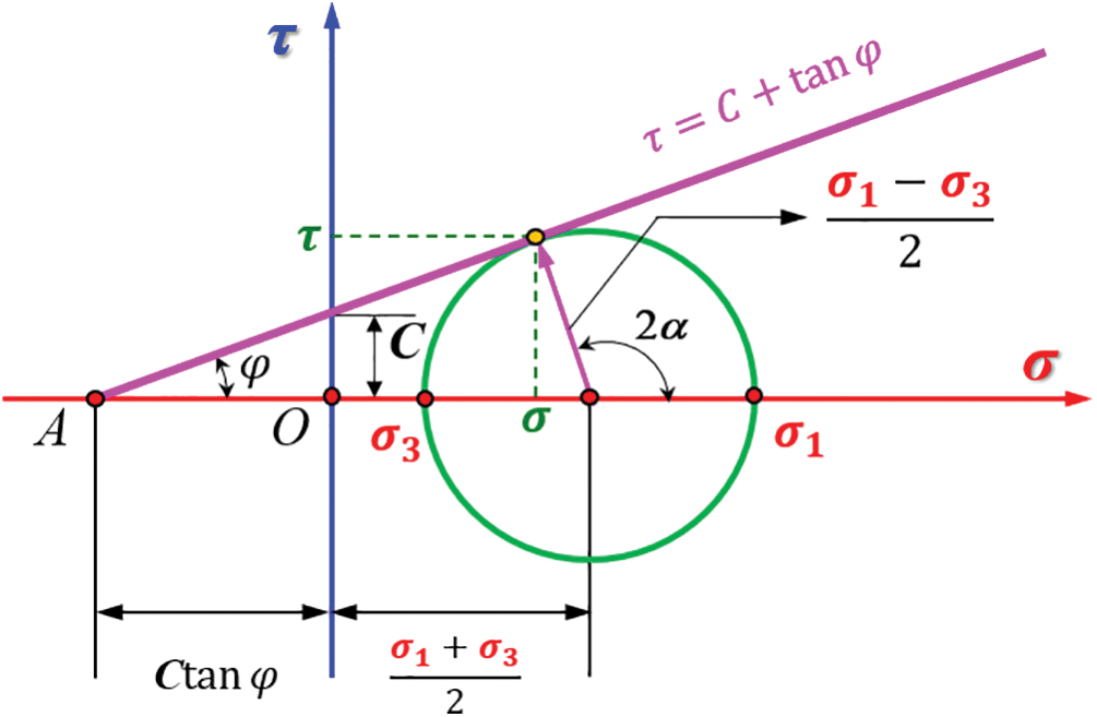
Figure 3: The schematic diagram of the Mohr Circle

3  Numerical Simulation for Wellbore Stability

Firstly, based on the theory of poroelasticity, a three-dimensional mechanical model of the wellbore is established through the finite element analysis method. And then, the three-way principal stresses at each point around the well perimeter are taken, and the rock’s state of damage is judged by the Mohr–Coulomb rock damage criterion. Finally, the coefficients of wellbore instability and wellbore stability are calculated.

3.1 Physical Model

3.1.1 Basic Assumptions of the Numerical Model

The key point of the study on the wellbore stability mechanical mechanism is the analysis of the stress state and stress distribution in the wellbore. Considering the effect of pore pressure changes during production on the effective stress of wellbore rocks, the mechanical analysis model obeys the following assumptions:

(1)   Rock initialization around the wellbore is assessed by using a pore elastic method with effective stress control for rock skeleton deformation and damage.

(2)   The numerical model obeys the elastic-plastic mechanics of porous media. When the damage occurs in the formation, the Mohr–Coulomb criterion is used for the strength criterion.

(3)   The percolation of the drilling fluid conforms to Darcy’s law. The effects of wellbore temperature variation and the geochemical reaction between drilling fluid and formation are ignored.

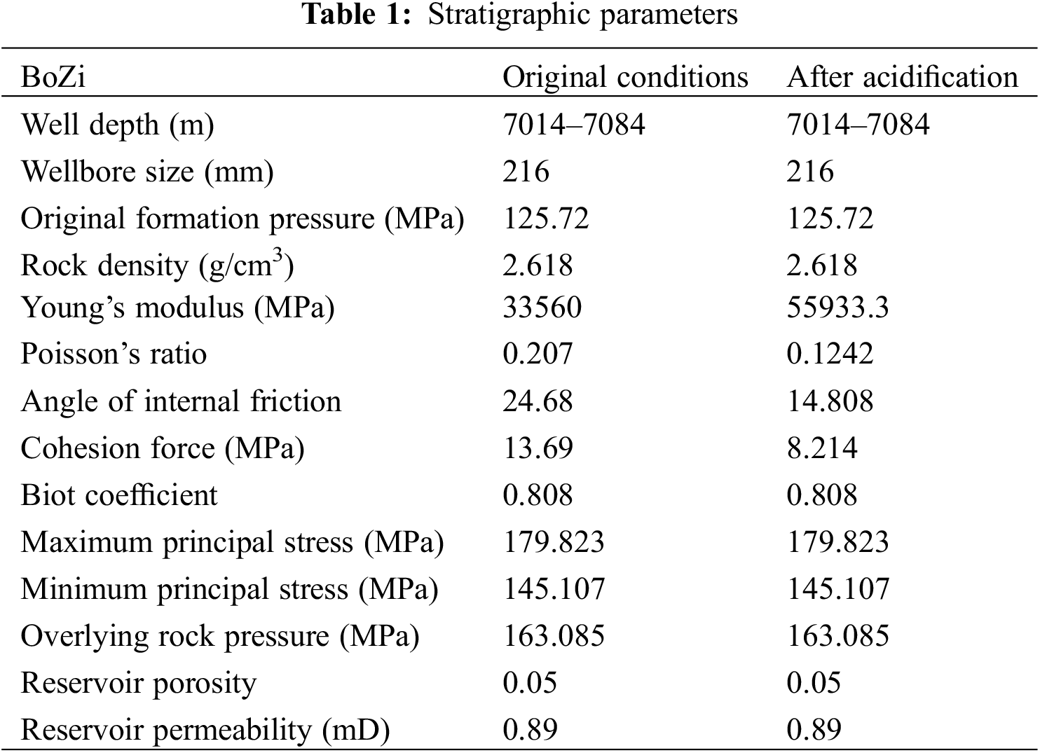
3.1.2 Numerical Model Parameters

BoZi is a normal-temperature and high-pressure gas reservoir located in northwest China. Referencing the BoZi formation properties, the two sets of geomechanical parameters are set to represent formation rock properties before and after acidification. The geomechanical parameters are presented in Table 1.

3.1.3 Finite Element Model of the Wellbore

As shown in Fig. 4, the formation model is a three-dimensional solid reservoir model with dimensions 160 m × 160 m × 80 m, around the wellbore with material properties. With drilling starting from the center of the x-y plane, a vertical well is drilled straight along the z-axis (i.e., overlying rock stress orientation). The wellbore diameter is 216 mm. To ensure the stability and accuracy of the solution, the grid setting strategy is shown in the table (Table 2) as follows:

Figure 4: Three-dimensional solid model

As shown in Fig. 5, underground engineering is a semi-infinite domain problem; the numerical simulation can only be performed in a limited range. Therefore, the model’s design must consider boundary effects, and a reasonable boundary condition is important to obtain reliable calculation results. The boundary conditions of this model are set to the original ground stress field and the original formation pore pressure. The maximum horizontal principal stress is 179.823 MPa, the minimum horizontal principal stress is 163.085 MPa, the overlying rock pressure is 145.107 MPa, and the original pore pressure is 125.72 MPa.

Figure 5: Mesh division

3.1.4 Model Calculation Process and Method

As shown in Fig. 6, the numerical calculation process is divided into three steps, detailed as follows:

(1)   Based on the stress balance theory, the original formation stress state of the numerical model is restored.

(2)   Using the cell deletion method, the cells in the wellbore are removed so that a wellbore can be formed. And the stress state of the wellbore will be refreshed by stress concentration.

(3)   The different production pressure is set and the pore pressure variation is simulated to clarify the change characteristics of pore pressure under different working conditions.

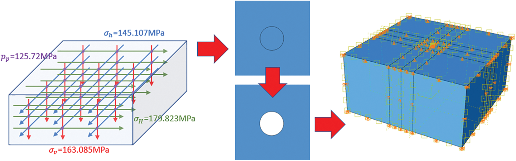
Figure 6: Model building and calculation process

3.2 Numerical Results and Discussions

3.2.1 Effect of Different Working Conditions on the Ground Stress

As the reservoir pore pressure decreases, there is insufficient fluid filling the pore of rocks, which causes the effective rock stress to increase, wellbore principal stress to change, and the gap between the maximum and minimum principal stress to be obvious. As shown in Fig. 7a, the minimum principal stress is 240 MPa and the maximum principal stress is 316.3 MPa before production. During the production with a 60 MPa pressure difference, the minimum principal stress is 39.65 MPa, and the maximum principal stress is 304.3 MPa (see Fig. 7b).

Figure 7: Principal stresses under different working conditions

In the original condition, the principal stress variation is mainly concentred on the four wellbore points at 0, 90, 180, and 360 degrees. The minimum principal stress extends uniformly outward along the circumference of the wellbore after production. And the maximum principal stress is mainly concentred on two points, at 0 and 180 degrees.

3.2.2 Effect of Production Pressure Difference on the Instability Coefficient of the Wellbore

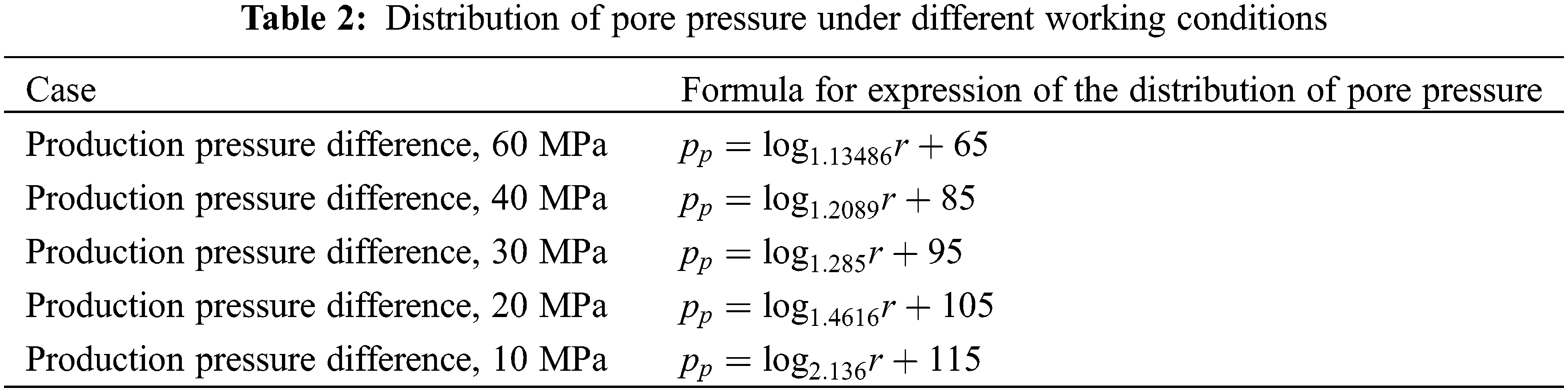
During Bozi reservoir production, the pore pressure shows a logarithmic distribution about the location of the wellbore center. The distribution rules are presented in Table 2.

The difference between the maximum and minimum principal stress is increased as the changes of principal stress in the wellbore. Comparing the scenario of 60 and 40 MPa production pressure difference (Figs. 8a and 8b), the wellbore instability coefficient is increased with the increase of production pressure difference, so the stable region has also expanded. Meanwhile, the wellbore instability coefficients at 10, 20, and 30 MPa are obtained by simulation calculation. The relationship curves of wellbore stability with well perimeter angle for different working conditions are obtained, as shown in Fig. 9. Overall, the risk of wellbore destabilization is greater as the production pressure difference increases as production progresses.

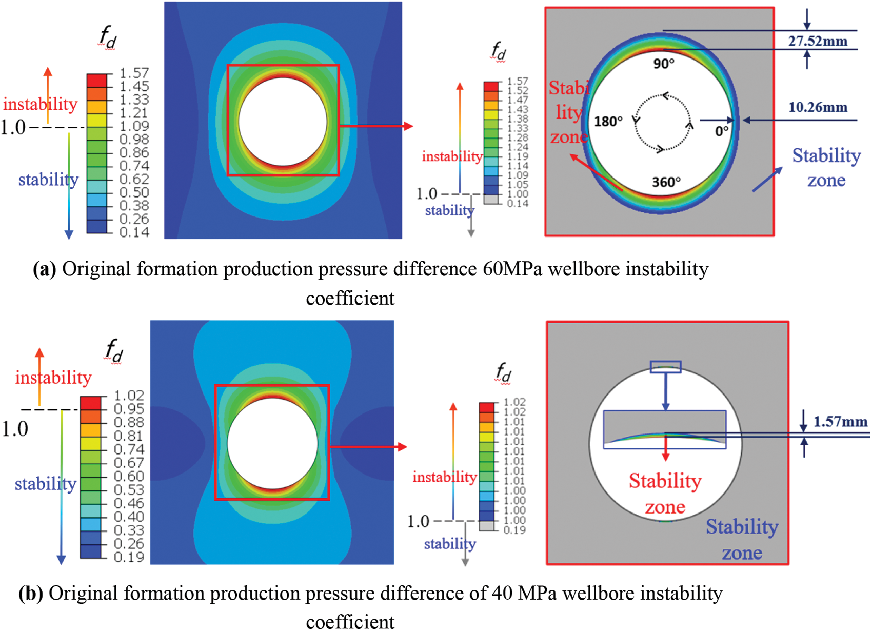
Figure 8: Wellbore instability coefficient for different working conditions. Under the 60 MPa production condition, the instability coefficients of the near wellbore are between 0.7 and 1.6. Under the 40 MPa, the same coefficients are between 0.5 and 1.0

Figure 9: Variation of wellbore instability coefficient with well circumference angle under original stratigraphy

3.2.3 Influence of Geomechanical Parameters on Wellbore Stability

After the acidizing operation, the formation rock mechanical strength decreases, the elastic modulus increases, and the Poisson’s ratio decreases. These will lead to an increased risk of wellbore destabilization. Fig. 10 shows the cloud plot of the change of wellbore stability coefficient at 60, 40, and 30 MPa, after acidizing the BoZi gas well. The threshold of wellbore instability after acidizing is reduced compared with the original formation, and the area of instability is further expanded under the same production pressure difference. The wellbore instability coefficients f 10 and 20 MPa production pressure differences are obtained through the simulation calculation. The maximum wellbore instability coefficient vs. well perimeter angle for different conditions after acidizing are obtained, as shown in Fig. 11. The wellbore instability coefficient and risk of wellbore instability are larger than the original formation under the same operating conditions.

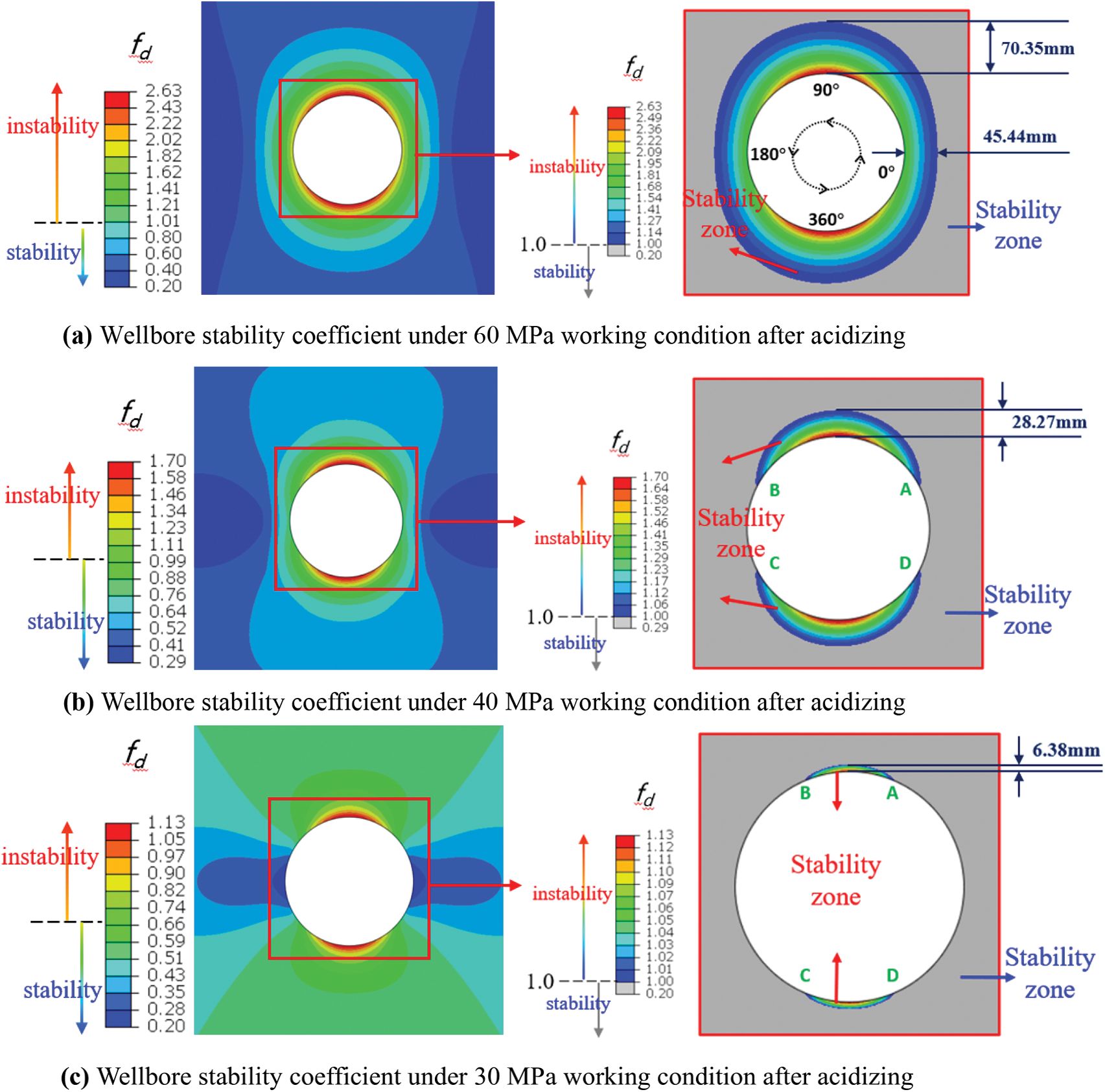
Figure 10: Wellbore instability coefficients for different geological conditions

Figure 11: Wellbore instability coefficient with well perimeter angle after acidification

4  Conclusions

(1)   The finite element analysis method with the Mohr–Coulomb rock damage criterion is used to establish finite element models for different working conditions and strata based on the theory of poroelasticity. The numerical simulation results reveal that different working and geomechanical conditions will affect the magnitude of the ground stress in the wellbore, increasing the risk of wellbore instability during production.

(2)   The model’s practicality is validated through the original formation and post-acidification conditions of the BoZi gas reservoir. With the increase of production pressure difference, the wellbore stability coefficient and the wellbore disability risk are increased in the original formation.

(3)   The acidised formation in the same production system has a bigger wellbore instability area and a lower production pressure difference threshold. In the on-site scenario, the numerical simulation results can help engineers choose a better production system for acidized formation production without the occurrence of wellbore instability accident.

Acknowledgement: None.

Funding Statement: This work is financially sponsored by Tarim Oilfield “Study on Adaptability Evaluation and Parameter Optimization of Completion Technology in Bozi Block, Tarim Oilfield” (Item Number: 201021113436).

Author Contributions: Study conception and design: Junyan Liu and Ju Liu; data collection: Yan Wang and Shuang Liu; analysis and interpretation of results: Shuang Liu, Qiao Wang, and Yihe Du; draft manuscript preparation: Yihe Du, Junyan Liu and Ju Liu. All authors reviewed the results and approved the final version of the manuscript.

Availability of Data and Materials: The data belongs to Tarim Oilfield which is very strict to the data security, as a result, for protecting the power requirements of Tarim Oilfield, the supporting data cannot be released.

Conflicts of Interest: The authors declare that they have no conflicts of interest to report regarding the present study.

References

1. Westergaard, H. M. (1940). Plastic state of stresses around a deep well. Journal of the Boston Society of Civil Engineers, 27(1), 1–5. [Google Scholar]

2. Braun, R. (2015). Wellbore stability-aspects of the influence of the 3D effective stresses. Oil Gas European Magazine, 41(3), 133–137. [Google Scholar]

3. Yew, C. H., Chenevert, M. E., Wang, C. L., Osisanya, S. O. (1990). Wellbore stress distribution produced by moisture adsorption. SPE Drilling Engineering, 5(4), 311–316. [Google Scholar]

4. Yu M., Chenevert M. E., Sharma M. M. (2003). Chemical–mechanical wellbore instability model for shales: Accounting for solute diffusion. Journal of Petroleum Science and Engineering, 38(3/4), 131–143. [Google Scholar]

5. Gomar, M., Goodarznia, I., Shadizadeh, S. R. (2014). Transient thermo-poroelastic finite element analysis of wellbore breakouts. International Journal of Rock Mechanics and Mining Sciences, 71, 418–428. [Google Scholar]

6. Gomar, M., Goodarznia, I., Shadizadeh, S. R. (2015). A transient fully coupled thermo-poroelastic finite element analysis of wellbore stability. Arabian Journal of Geosciences, 8, 3855–3865. [Google Scholar]

7. Ding, L. Q., Lv, J. G., Wang, Z. Q., Liu, B. L. (2022). Wellbore stability analysis: Considering the upper limit of shear failure criteria to determine the safe wellbore pressure window. Journal of Petroleum Science and Engineering, 212, 110219. [Google Scholar]

8. Lu, Y. H., Chen, M., Jin, Y., Zhang, G. Q. (2012). A mechanical model of wellbore stability for weak plane formation under porous flow. Petroleum Science and Technology, 30(15), 1629–1638. [Google Scholar]

9. Ding, L. Q., Wang, Z. Q., Liu, B. L., Wang, Y. (2019). Wellbore stability analysis: A new model considering the effects of anisotropic permeability in bedding formation based on poroelastic theory. Journal of Natural Gas Science and Engineering, 69, 102932. [Google Scholar]

10. Jin, Y., Chen, M., Liu, G. H. (1999). Mechanical analysis of wellbore stability in large displacement wells. Journal of Geomechanics, (1), 6–13. [Google Scholar]

11. Zou, L. Z., Deng, J. G., Zeng, Y. J. (2008). Pre-drill water formation prediction and wellbore stability study for gas drilling. Petroleum Drilling Techniques, 36(3), 46–49. [Google Scholar]

12. Tang, G., Gong, H., Xu, J. N., Zhou, L., Zhang, H. L. et al. (2022). Well wall stability experiment for completion test of Permian Yong Tan 1 volcanic gas well in Sichuan Basin. Natural Gas Industry, 42(3), 91–98. [Google Scholar]

13. Ding, Y., Liu, X. J., Luo, P. Y., Liang, L. X. (2018). Study of wellbore stability in hard and brittle mud shale formations. China Offshore Oil and Gas, 30(1), 142–149. [Google Scholar]

14. Liang, L. X., Ding, Y., Liu, X. J., Xu, L. (2016). Study on the coupling of stable seepage—Mechanization in hard and brittle mud shale wellbore stability. Special Oil and Gas Reservoirs, 23(2), 140–143+158. [Google Scholar]

15. Zhu, K. L., Wu, X. H., Jia, S. P., Lv, F., Xiao, Z. Q. (2019). Dynamic damage analysis of mud shale wellbore under force-chemical coupling. Journal of Guangxi University (Natural Science Edition), 44(4), 1052–1061. [Google Scholar]

16. Wang, D. B., Qu, Z., Ren, Z. X., Shan, Q. L., Yu, B. et al. (2022). Numerical simulation on borehole instability based on disturbance state concept. Energies, 15(17), 6295. [Google Scholar]

17. Gao, J. J., Lin, H., Sun, J., Chen, X. P., Wang, H. X. et al. (2022). A porothermoelastic model considering the dynamic temperature-perturbation boundary effect for borehole stability in fractured porous rocks. SPE Journal, 27(4), 2491–2509. [Google Scholar]

18. Wei, Y. R., Feng, Y. C., Deng, J. G., Li, X. R. (2021). Hydro-mechanical modeling of borehole breakout in naturally fractured rocks using distinct element method. Geomechanics for Energy and the Environment, 31, 100287. [Google Scholar]

19. Mao, L. J., Lin, H. Y., Cai, M. J., Zhang, J. (2022). Wellbore stability analysis of horizontal wells for shale gas with consideration of hydration. Journal of Energy Resources Technology, 144(11), 113003. [Google Scholar]

20. Li, X., Zhang, J., Li, C. N., Chen, W. L., He, J. B. et al. (2022). Characteristic law of borehole deformation induced by the temperature change in the surrounding rock of deep coalbed methane well. Journal of Energy Resources Technology, 144(6), 111217. [Google Scholar]

21. Jin, Y., Chen, M. (2012). Wellbore stability mechanics. Beijing, China: Science Press. [Google Scholar]

22. Liu, X. J., Luo, P. Y. (2004). Rock mechanics and petroleum engineering, pp. 118–128. Beijing, China: China Petroleum Industry Press. [Google Scholar]

23. Fairhurst, C. (1968). The phenomenon of rock splitting parallel to a free surface under compressive stress. Proceedings of the 1st Congress of the International Society of Rock Mechanics, Lisbon. [Google Scholar]

24. Zhao, X. L. (2008). Study on wall stability of arbitrary wellbore in oil drilling. Chongqing, China: University of Chongqing. [Google Scholar]