Numerical Simulation of Slurry Diffusion in Fractured Rocks Considering a Time-Varying Viscosity

1  Introduction

The presence of rock fissures reduces the strength of a rock mass, leading to instability of the surrounding rock and groundwater gushing out. The grouting of fractured rock mass is a technology to improve the mechanical properties of rocks and prevent groundwater seepage, thereby ensuring the safety of engineering constructions. Grouting involves injecting a slurry with high grouting pressure into fissures, connecting the rock matrix and weakening groundwater flow [1,2]. The grout penetration length is a critical parameter for evaluating the effect of crack grouting, which determines the actual scope of grouting reinforcement and affects the project quality and construction cost. When seepage diffusion is too large, resources are wasted, increasing costs incurred, whereas effective reinforcement cannot be achieved when it is too small [3,4]. Thus, it is crucial to understand the factors affecting the grouting effect and study the grout penetration range, as shown in Fig. 1.

Figure 1: Grouting effect diagram

Several researchers have conducted in-depth research on the modeling of rock fracture penetration. Regarding theoretical research, Wallner [5] calculated the analytical solution of penetration length in a one-dimensional fracture model channel based on the Bingham’s fluid flow theory, considering the influence of the viscosity and yield strength of the slurry. Wereley et al. [6] proposed the steady laminar flow equation of an incompressible Bingham fluid in smooth parallel fractures. Lombardi [7] deduced the relationship between slurry flow and penetration length based on the single fracture grouting model. Yang et al. [8,9] derived a relation for calculating the effective penetration radius and diffusion of slurry in sand using the power law and Bingham’s model. Yang et al. [10] derived the relation for the penetration length of a Bingham slurry grout based on the slurry rheological and seepage equations.

The aforementioned theoretical studies were based on the fixed initial viscosity value or considered the influence of the time dependence of the slurry in a single fracture model. In this way, the calculated theoretical penetration length was larger than the measured value in the grouting process. Li et al. [11] experimentally measured the time-varying apparent viscosity of a cement-water glass slurry. Ruan [12] developed a time-varying fracture diffusion model through many experimental calculations and obtained the relationship between the slurry water-cement (W/C) ratio and rheology. Zhao et al. [13] analyzed the relation between the hydro-mechanical (HM) coupling and investigated the stability of water-resistant rock pillars using the strength reduction method, and the factor of safety (FOS) of the pillar was established. Saada et al. [14,15] conducted laboratory tests to study the diffusion mechanism of one-dimensional grouting and obtained the influence of infiltration effect on grouting infiltration. Liu et al. [16] and Zhao et al. [17] obtained the slurry-water interface function using the quasi-three-dimensional grouting system. The water-force coupling tests were carried out under varying differential water pressure and confining pressure conditions to obtain stress-strain penetration characteristics. Since field or laboratory tests are easily affected by test conditions, it is difficult to capture the slurry flow accurately. Thus, studying the fracture grouting seepage process based on numerical simulation is becoming one of the most economical and practical methods.

Numerical simulation methods can provide better accuracy and relatively less time and cost requirements for studying fluid flow. The two main methods currently used in fracture grouting simulation tests are the finite element method (FEM) and the discrete element method (DEM). Based on the FEM, Eriksson et al. [18] studied the grouting flow in fractures based on the one-dimensional fracture model. Chen et al. [19] combined the FEM and volume of fluid (VOF) methods to simulate the diffusion process of splitting grouting. The main factors for controlling slurry flow in rock mass were numerically studied by Xiao et al. [20], and the influencing factors of grout penetration length were obtained. Wang et al. [21,22] deduced through numerical simulations that grouting pressure, W/C ratio, and hydraulic opening play a critical role in the grouting diffusion range. Based on the one-dimensional fracture grouting model, Lee et al. [23] studied the influence of the penetration of fractured rock mass on the grouting reinforcement effect and extended it to a two-dimensional model. Based on the DEM, Saeidi et al. [24] suggested a numerical model for predicting the grouting amount and the penetration length into joints and studied the rock mass properties and their influence on the grouting penetration length. Liu et al. [25] studied the grouting diffusion mechanism based on the principle of the plane model by combining the finite discrete element method (FDEM) with the grouting flow simulator and considering the aperture change due to HM coupling. Combined with the geology of a dam, Mortarazavi et al. [26] analyzed the influence of grouting pressure, hydraulic opening, joint trace length, and opening on the grouting effect using a numerical simulation system. Liu et al. [27] proposed a numerical manifold method (NMM) for simulating the grouting penetration process of fractured rock mass by assuming that the flow characteristics of the slurry are that of a Bingham fluid. Based on the NMM, Liu et al. [28] proposed an NMM-HM grouting model for studying slurry flow and grouting effect analysis. Mohajerani et al. [29] used a two-dimensional fracture network to numerically simulate the grouting factors, such as grouting pressure, density, and grouting time affecting slurry diffusion. Pan et al. [30] put forward an analytical solution considering the excavation failure zone. Likewise, Zhao et al. [31] proposed a dual-medium model, including equivalent continuous and discrete fracture media, to study the coupled seepage-damage effect in fractured rock masses. Yang et al. [32] numerically simulated the whole process of a Bingham fluid in fracture grouting based on the random fracture network. The study did not further consider the time-varying of the slurry itself and simulated the constant initial viscosity; some assume that the rock mass around the fracture is a rigid body, and the fracture aperture remains unchanged during the grouting process. However, in the actual grouting process, the slurry viscosity is normally proportional to time, and the grouting pressure also affects the fracture aperture.

Therefore, because of the identified research gaps, a time-varying experimental study on the viscosity of slurries with different W/C ratios was conducted in this paper to determine the change in viscosity with time. A fluid-solid coupling model of grouting diffusion with time-varying viscosity was established based on the DEM and Bingham fluid constitutive equation. Finally, the numerical simulation was validated by a theoretical solution. Based on different fracture forms (single fracture, branch fracture, and fracture network), the influence of time-varying slurry viscosity and fracture aperture change on the grouting penetration effect were discussed, and the whole process of viscosity time-varying was simulated by adjusting the model.

2  Time-Varying Viscosity Test on the Cement Slurry

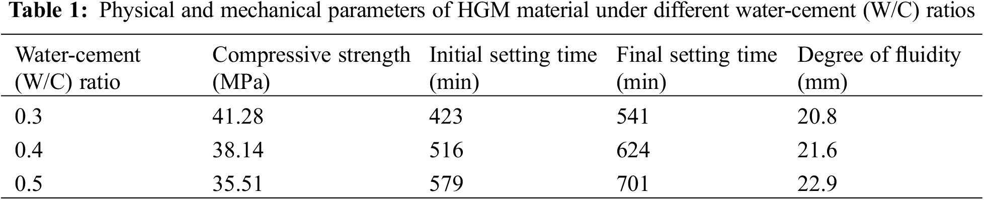
In this study, a composite slurry (HGM) developed independently by the same research group was used. The physical and mechanical parameters of the HGM materials with varying W/C ratios are presented in Table 1. At 0.3 W/C ratio, the maximum uniaxial compressive strength of the hardened (hydrated) cement slurry was determined as 41.28 MPa, with initial setting time, final setting time, and fluidity of 423, 541 min, and 20.8 mm, respectively. As the Water-cement ratio increased, the strength of the hardened cement slurry decreased, the setting time increased, and the fluidity increased.

The NDJ-9S rotary digital display viscometer was used to measure the time-varying parameters of the cement slurry. The instrument controls the smooth operation of the motor according to the set speed and drives rotor rotation through the wire. In the absence of resistance, the rotor and motor rotate synchronously. When the rotor encounters liquid resistance, its rotation lags behind that of the motor. When the tension of the spring wire and the measured liquid resistance acting on the rotor are balanced, the opening angle of the lagging motor of the rotor becomes fixed. By measuring this opening angle, the instrument calculates the viscosity of the measured liquid and displays it on the LCD screen.

In this study, the HGM cement slurry was evaluated for viscosity values at the same mineral composition ratio and varying W/C ratios. The HGM cement slurries were prepared at three W/C ratios of 0.3, 0.4, and 0.5. The No. 3 rotor was selected at a speed of 30 rpm for the slurry with W/C ratio of 0.3, the No. 3 rotor was selected at 60 rpm for the slurry with W/C ratio of 0.4, and the No. 2 rotor was selected at 30 rpm for the slurry with W/C ratio of 0.5. The test setup and details are shown in Fig. 2.

Figure 2: Flow chart of slurry preparation determination

The viscosity variation curve of the cement slurries with time was plotted and is shown in Fig. 3a. The viscosity of the HGM slurry at the different W/C ratios increased with time, indicating delayed growth in the early stage and rapid growth after the pumpable period. The viscosity change points under the three W/C ratios corresponded to 6, 9, and 12 min. The viscosity evolution curve with time was divided into the early growth hysteresis as the growth hysteresis zone and the later stage as the rapid growth zone. As the W/C ratio increased, the viscosity decreased, and the growth rate slowed. When the W/C ratio was increased from 0.3 to 0.5, the initial viscosity decreased from 1.312 to 0.432 Pa⋅s, and the time of the viscosity hysteresis zone increased from 10 to 17 min. This change occurred because the HGM cement slurry maintained good fluidity viscosity during the pumpable period. The viscosity rapidly increased after the pumpable period, initiating solidification to achieve the grouting plugging effect.

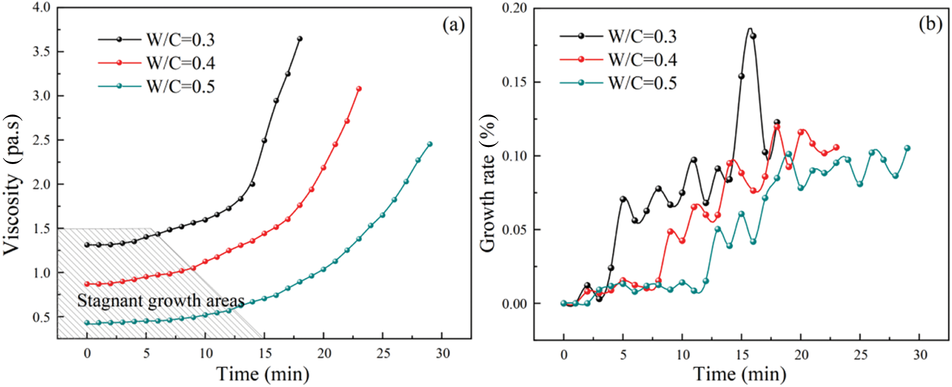
Figure 3: Relationship between viscosity and viscosity growth rate with time: (a) Viscosity; (b) viscosity growth

The trend of HGM slurry viscosity changed with time under different W/C ratios and exhibited a positive correlation, with varying viscosity growth values at different times. In order to investigate the relationship between viscosity changes before and after the pumpable period under different W/C ratios, the concept of viscosity growth rate was introduced, as given in Eq. (1):

ω=μt−μt′μt (1)

where ω is the rate of increase in viscosity; μt is the viscosity value at a certain moment; μt′ is the viscosity value at the previous moment.

As shown in Fig. 3b, the time-varying viscosity exhibited different growth rates with time. Before the 5-min mark, the viscosity growth rates of the three slurries with different W/C ratios did not significantly change. After reaching the viscosity change point before the pumpable period, the growth rate fluctuations increased for the slurries with varying W/C ratios. The viscosity growth rate of the HGM slurry with a W/C ratio of 0.3 reached 0.18 after 6 min, while the rate for the HGM slurry with a W/C ratio of 0.4 reached 0.12 after 9 min. Similarly, the rate for the HGM slurry with a W/C ratio of 0.5 reached 0.10 after 12 min.

The growth rate curve signified early stability. The growth rate increased wave-likely when the slurry reached the rapid growth zone after the growth lag period. Slurries with low W/C ratios reached the maximum wave peak first, indicating that the increased W/C ratio reduced the increasing rate of viscosity. Consequently, the time it took to reach the viscosity change point and the speed at which the slurry reached the viscosity peak decreased.

Based on the exponential function y=a+becx fitting of the viscosity-time curve of the HGM cement slurry at different W/C ratios, the time-varying equation of viscosity at the different W/C ratios was obtained as presented in Eq. (2).

{μ(t)=1.333+0.02e0.268t  W/C=0.3μ(t)=0.885+0.05e0.165t  W/C=0.4μ(t)=0.395+0.05e0.128t  W/C=0.5 (2)

where μ(t) is the viscosity time function (Pa⋅s), and t is time (min).

The comparison was made with the actual test values by selecting the time t = (0, 5, 10, 15, 20, 25) and using the fitting equation to calculate the slurry viscosity value under each W/C ratio condition. The results are shown in Fig. 4.

Figure 4: Comparison of fitting value and test value of different W/C ratios: (a) W/C = 0.3; (b) W/C = 0.4; (c) W/C = 0.5

The close alignment between the test data and the fitted values, as depicted in Fig. 4, shows the reliability and accuracy of the fitting equation. The maximum difference between the fitted and test values was 0.057 Pa⋅s, with an error of 14.4%. Most of the remaining data values fell within a 5% range, which not only demonstrated the effectiveness of the fitting function but also confirmed that the viscosity evolution of the HGM cement slurry over time adhered to the formation of μ(t)=a+becx .

3  Fluid-Solid Coupling Model of Viscosity Time-Varying Grouting Diffusion

3.1 Bingham Fluid Flow Theory

(1)   Constitutive equation

The Bingham fluid is a viscoelastic non-Newtonian fluid with a higher yield strength τ0 , and the fluid only begins to flow when it reaches the minimum shear stress. Below the critical value τ0 , it exhibits the behavior of an ordinary elastomer. The relationship between the shear stress and shear rate of the slurry is given as Eq. (3) [33,34].

τ=τ0+μγ (3)

(2)   Diffusion equation

As shown in Fig. 5, the Bingham fluid flow model contained two regions. i.e., the plug flow region and the velocity gradient region. In the plug flow region, the slurry moves as a whole and has the same velocity. Since the shear stress was less than the yield strength, the velocity gradient in the plug flow region did not exist. In order to ensure the grouting feasibility, the height of the plug flow area must be less than the crack aperture. The gray part of the plug flow area of the flow model was analyzed, and the equilibrium equation developed is given as Eq. (4).

bdp+2τdr=0 (4)

where dr is the length of the micro-unit, dp is the pressure increment, and b is the height of the micro-unit.

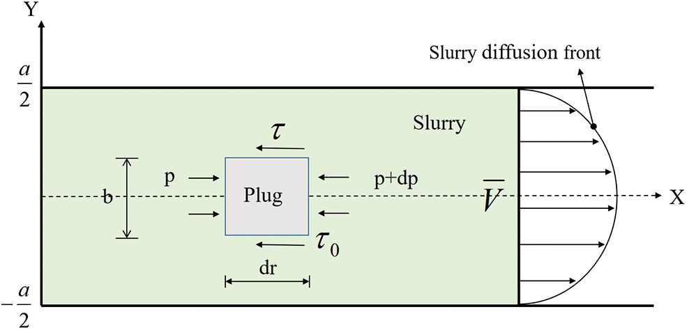
Figure 5: Bingham grout fluid model

The plug flow interval height formula was calculated by the equilibrium equation as given in Eq. (5).

b=−2τdrdp (5)

Considering that the height of the plug flow zone must be less than the crack aperture, else, the slurry cannot flow, Eq. (5) is transformed to Eq. (6).

2τ0b≤−dpdr (6)

Eq. (6) shows that there was a pressure gradient ( J=2τ0/b ) in the slurry movement of Bingham fluid slurry due to shear stress.

From Eq. (3), the shear stress is given as Eq. (7) outside the plug flow region.

τ=τ0+μ(−dvdb)=−b2dPdr (7)

Eq. (7) can be further written as Eq. (8).

dvdx=1μ(b2dPdr+τ0) (8)

The integral of Eq. (8) yields Eq. (9).

v=1μ(dpdrb24−τ0b)+C (9)

where C is the constant of integration.

In the velocity gradient interval, the velocity of the Bingham fluid changes along the direction of fracture height. According to the flow differential equation and boundary condition in Eq. (6), the average velocity of the slurry was obtained as given in Eq. (10).

V¯=a212μ[−dpdx+3τ0a(−dp/dr)−4τ03a3(−dp/dr)2] (10)

where τ is the shear stress of the slurry; τ0 is the yield shear stress of the slurry; μ is the slurry viscosity; γ=−(dv/dy) is the shear rate ( v is the slurry flow velocity, y is vertical slurry flow direction distance); b is the width of plug flow zone; a is the aperture width; p is the grouting pressure.

3.2 UDEC Fluid Flow Model

UDEC (Universal Distinct Element Code), a well-known discrete element code software for rock mechanics, imposes no restrictions on fluid types, allowing for the reasonable simulation of fluids in any flow state [35,36]. It can analyze fluid flow in scenarios with impermeable cracks between blocks and effectively conduct HM coupling analysis. The fluid conductivity within the structural plane depends on the mechanical deformation of that plane. Conversely, the fluid pressure within the structural plane also impacts the calculation. Fig. 6a shows the fluid-solid coupling diagram in UDEC.

(1)   Aperture width

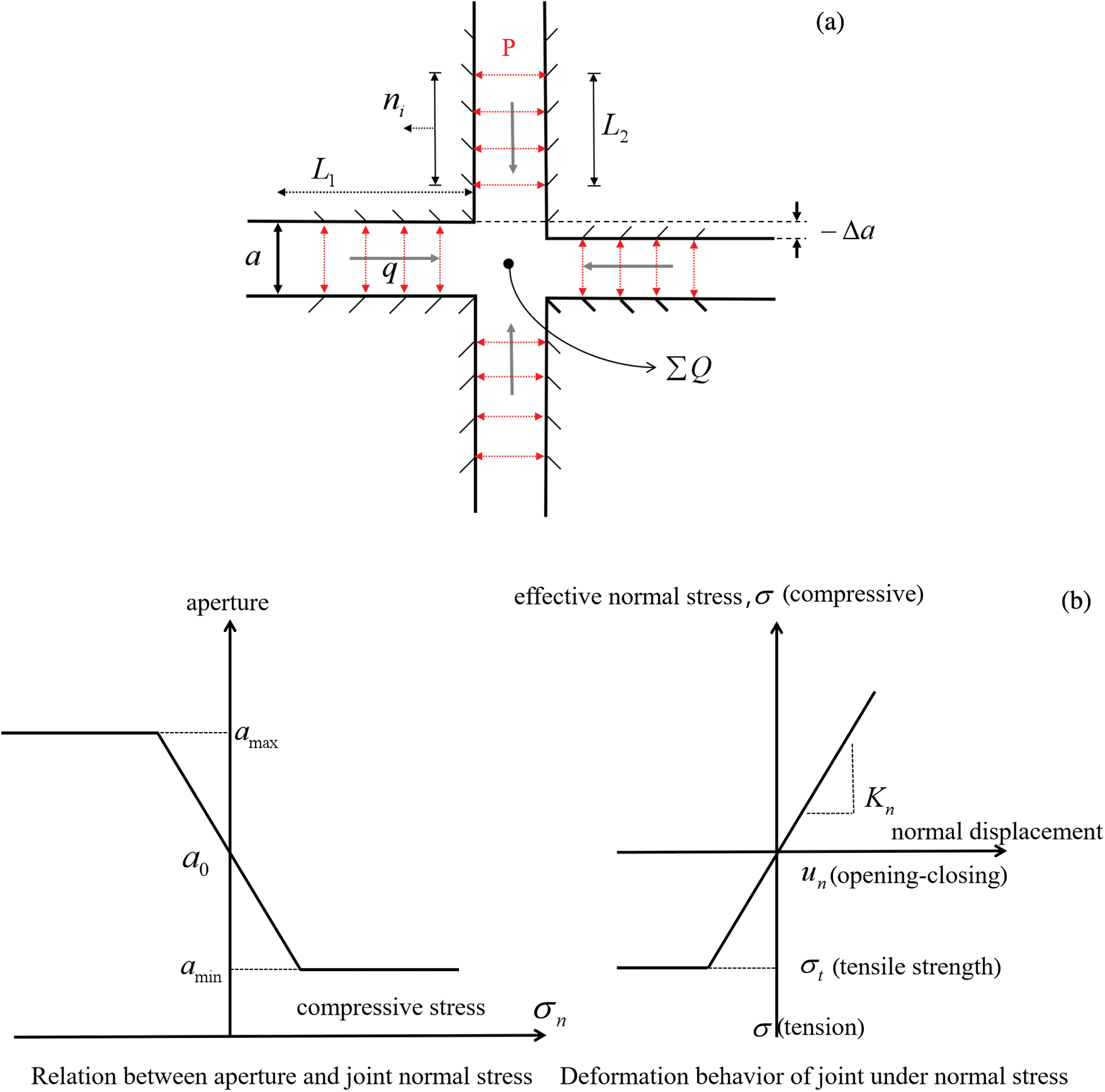
Figure 6: UDEC percolation model: (a) Fluid-solid coupling; (b) aperture and joint deformation in relation to normal stress

The flow of fluid is accompanied by the change in aperture width. The flow velocity of the fluid is updated based on the change in aperture width. The influence of the mechanical deformation of the joint surface on the fluid pressure mainly depends on the normal stiffness of the joint. According to Barton et al. [37], the effective aperture expression is given as Eq. (11).

a=a0+Δun (11)

where a0 denotes the aperture when there is zero normal stress and Δun is the tensile or compressive force applied to the joint that leads to an increase in the aperture in the form of opening or closing.

As shown in Fig. 6b, the relationship between the aperture and the joint deformation with the normal stress is given. The minimum aperture amin does not affect the penetration of the contact. A maximum aperture amax (generally 5 times the aperture value) is also assumed in the model calculation. The slope of the relationship between the effective normal stress and the normal displacement is taken as the normal stiffness. Kn is a constant, which can be directly assigned from the parameters. In addition, the tensile strength σt has little effect on the deformation and does not affect the flow of the slurry.

(2)   Pressure generation

In the UDEC calculation model, new joint geometry is generated with increased grouting pressure, resulting in new aperture and flow volume values. The pressure in the new area after Δt is obtained as given in Eq. (12) [38].

p=p0+KQΔtV−KV−V0Vm (12)

where p0 is the regional pressure for the previous time step; K is the bulk modulus of the slurry; Q is the volume of the regional slurry; V and V0 are the areas of the current region and the previous region, respectively; Vm=(V+V0)/2 .

4  Viscosity Time-Varying Model and Algorithm Based on UDEC

In rock mass grouting, the time-varying related problems in the rheology of the slurry are usually considered. In order to better reflect the time-varying nature of the slurry in the grouting process under actual conditions, a fluid-solid coupling algorithm model of the viscosity time-varying grouting diffusion was built based on UDEC numerical simulation. Determining the slurry flow pattern was the basis for establishing the grouting diffusion model. Based on rheological characteristics, the fluid flow pattern was divided into power-law fluid, Newtonian fluid, and Bingham fluid. The research findings on slurry flow patterns and rheological equation [39] indicate that cement-based slurries, such as cement clay slurry, cement composite slurry, and polymer cement slurry, are generally Bingham fluids. In studying the grouting diffusion of cement slurry, most researchers have mainly focused on Bingham fluids. By combining the properties of slurries and rheological equations, it was determined that the flow pattern of the HGM slurry (used in this study) depicted the Bingham fluid. The main innovation of this model is that the change of viscosity accompanied the calculation process, and the law of viscosity change was strictly following the time-varying characteristic function of experimentally-measured viscosity. A viscosity time-varying coupling model was developed for the Bingham fluid HGM slurry. The basic assumptions and prerequisites for establishing the model are given as follows:

1) The slurry is an incompressible, homogeneous, and isotropic liquid.

2) The flow pattern remains unchanged as the slurry flows through the aperture.

3) The rock wall surface is impervious, preventing water from the slurry from penetrating the rock wall; thus, it is considered that the slurry flows only within the aperture.

4) The slurry diffusion in the fracture is a complete drive diffusion, ignoring the diluting effect of the slurry-water interface on the slurry.

5) The time-varying slurry has good injectability and will not cause clogging.

6) Before the slurry reaches its yield strength, grouting can be repeated.

4.1 Viscosity Time-Varying Constitutive Equation

Under a constant grouting rate, the slurry viscosity at the grouting hole remained constant. In the theoretical model of fracture grouting, the time when the slurry entered the aperture channel from the grouting hole was considered the starting point for slurry viscosity growth, meaning that the viscosity at the grouting hole corresponded to the initial viscosity of the HGM slurry. According to the law of conservation of mass, the total amount of slurry injected equals the flow diffused within the fracture. The relationship between the slurry penetration length and grouting time is given by Eq. (13).

qt=2πa(r2−ra2) (13)

where q is the grouting rate, a is the aperture width, rt is the grout penetration length at time t, and ra is the radius of the grouting hole.

The grouting hole was very small relative to the entire slurry diffusion area. Ignoring the grouting hole radius, Eq. (13) could be identically transformed to obtain the grout penetration length as given in Eq. (14).

r=qt2πa (14)

During grouting, the viscosity change involves three time concepts. The total grouting time t is based on the start and end of grouting. The slurry starting flow time ts refers to when the slurry begins to flow when it enters the fracture channel to reach the yield stress strength. The slurry viscosity growth time tg is based on the slurry start flow time as the starting point and the grouting end time as the endpoint. Thus, the total grouting time can be written as Eq. (15).

t=ts+tg (15)

Substituting Eq. (15) into Eq. (13) gives Eq. (16).

q(ts+tg)=2πa(r2−ra2) (16)

During the whole grouting time, the slurry flow time was much smaller than the slurry viscosity growth time and the total grouting time. Ignoring the grouting hole radius, Eq. (16) can be simplified as given in Eq. (17).

tg=2aπr2q (17)

When the grouting time is t, the slurry viscosity corresponding to the penetration length r is given as Eq. (18).

μ(r, t)=μ(tg) (18)

Substituting Eq. (17) into Eq. (18) gives the time-varying distribution equation of viscosity, as given in Eq. (19).

μ(r, t)=μ(2aπr2q) (19)

It is well-known that the yield stress of cement slurry does not change much with time [12], which can be regarded as time-invariant, so τ0(t)=τ0(0)=τ0 . The time-varying viscosity function was integrated into the Bingham fluid rheological equation to obtain the time-varying HGM slurry rheological equation (Eq. (20)).

τ(t)=τ0+μ(2aπr2q)γ (20)

4.2 Viscosity Time-Varying Diffusion Equation

In the grouting process, according to the constant quality of the slurry, the grouting rate satisfies Eq. (21).

q=4πrav¯ (21)

Throughout the grouting process, −dp/dx was much larger than the starting pressure J=2τ0/b . Ignoring the high-order small terms in Eq. (10) and substituting Eq. (21) into Eq. (10) gives leads to Eq. (22).

V¯=a212μ(2aπR2q)(−dpdr)[1−3τ02a(−dp/dr)](r≤qt2πa) (22)

The pressure change equation of the slurry diffusion zone was obtained by substituting Eq. (21) into Eq. (22) to give Eq. (23).

dpdr=3qπa31rμ(2aπr2q)+3τ02a (23)

Eq. (23) was integrated within the diffusion region (r, rt) and brought into the boundary condition (r=rt) to obtain the pressure distribution equation in the slurry diffusion region, as given in Eq. (24).

p(r, t)=3qπa3∫Rqt2πa1rμ(2πar2q)dr+3τ02a(qt2πa−r)(r≤qt2πa) (24)

When (r=r0) , the grouting pressure was given by P=p(r0, t) . Then, the relationship between grouting pressure and time was obtained by integrating it into Eq. (24) to give Eq. (25).

P=3qπa3∫r0qt2πa1rμ(2πar2q)dr+3τ02a(qt2πa−r0) (25)

Substituting the slurry diffusion radius rt=qt/2πa into Eq. (25), the relationship between the grouting pressure and slurry penetration length was obtained as given in Eq. (26).

P=3qπa3∫r0rt1rμ(2πar2q)dr+3τ02a(rt−r0) (26)

In the UDEC numerical model, the viscosity parameter is a hidden parameter and cannot be directly assigned. In order to reflect the time-varying viscosity, the penetration coefficient of the joint contact surface was modified to simulate the flow of plastic fluid. UDEC presented the relationship between the penetration coefficient and the viscosity of the joint surface as given in Eq. (27).

kj=112μ (27)

Based on the UDEC flow model, the relationship between the average flow velocity and the penetration coefficient of the slurry in the HGM viscosity time-varying model was obtained by substituting the formula into Eq. (27) to give Eq. (28).

V¯=a2kj(2aπr2q)[−dpdr+3τ02a](r≤qt2πa) (28)

The slurry flow per unit time is given by Eq. (29).

Q=V¯⋅a=a3kj(2aπr2q)[−dpdr+3τ02a](r≤qt2πa) (29)

The relationship between grouting pressure and penetration length in the time-varying model of HGM viscosity was obtained by substituting Eq. (27) into Eq. (26) to give Eq. (30).

P=3qπa3∫r0rt1r12kj(2πar2q)dr+3τ02a(rt−r0) (30)

Fig. 7 shows the algorithm process of the viscosity time-varying model. First, the model size and the crack form were determined. The model was drawn, and the crack was generated using the language editing function of UDEC. The corresponding material properties were assigned. The boundary conditions of the model were set, and initial conditions were loaded, eliminating any changes resulting from the loading of initial conditions.

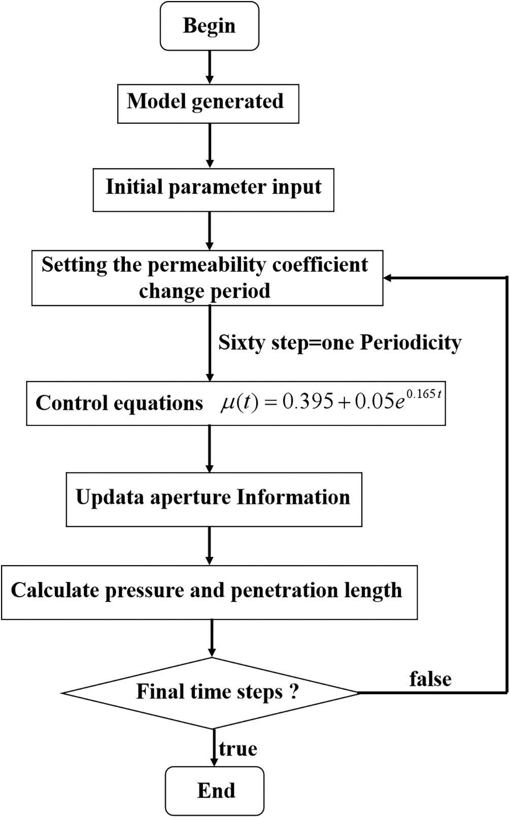
Figure 7: Flowchart of the calculation in the viscosity time-varying algorithm model

The core part of the model was incorporating the time-varying algorithm. UDEC simulated the entire grouting process with a constant penetration coefficient, which did not accurately represent the actual situation. Building on the UDEC flow model, the UDEC step number 1 corresponded to the actual grouting time of 1 s, while step number 60 represented one calculation cycle. From Eq. (27), the fracture penetration coefficient was given to characterize the initial viscosity value of the cement slurry. Using FISH language, the viscosity value of the cement slurry was changed at step number 60 in each cycle. The corresponding slurry punching surface viscosity value is shown in Fig. 8. This strictly adhered to Eq. (2) in characterizing the viscosity time function change, accommodating the slurry’s time-varying nature during the grouting process.

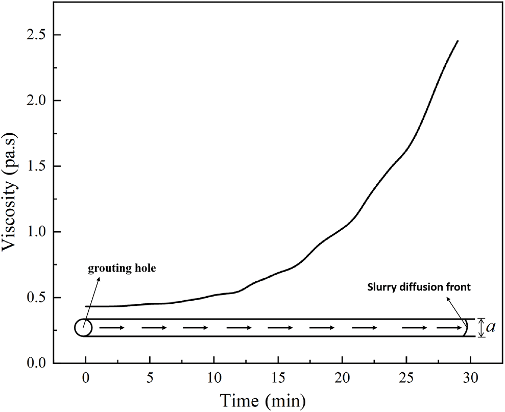
Figure 8: Viscosity plot of the slurry diffusion front

The fluid function in the fluid model was activated, and fluid material properties were assigned. The density, yield stress, and bulk modulus were provided to calibrate the cement slurry under consideration. A constant grouting pressure design value of 2 MPa was assigned to the grouting hole for the grouting test. The penetration length data and the cloud diagram of the fracture width change were the output. The relationship between grouting pressure and penetration length was calculated using Eq. (30).

5  Model Verification and Simulation of Grouting

The numerical simulation in the UDEC software was influenced by the response of the discontinuous medium (rock joints) under static or dynamic loads. The discontinuous medium in UDEC comprised a combination of discrete element blocks, with discontinuity serving as a constraint condition between blocks. This enabled the simulation of pores within the model and fluid flow issues on discontinuous surfaces. The types of fluid flow in UDEC were divided into complete rock bodies and structural planes. The fluid flow in structural planes was investigated in this study.

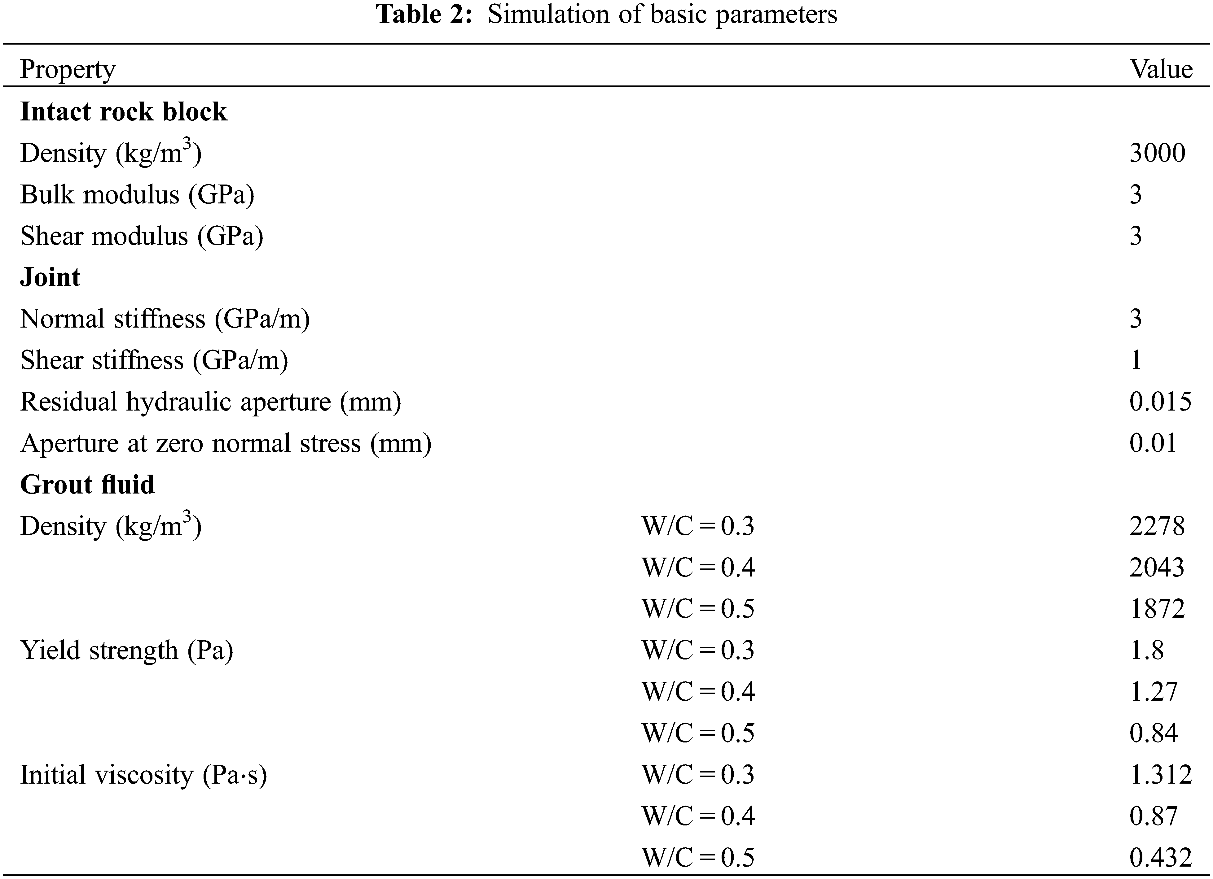
There are three main methods used for generating the UDEC joints–(i) using the system language to edit and divide rock blocks to create joints, (ii) generating random joints based on Voronoi, and (iii) importing the required joint forms with the assistance of CAD drawing software. Ma et al. [40] and Zhao et al. [17] studied the different mechanical properties of their samples by changing the W/C ratios in laboratory tests. It was shown that the strength of the resulting samples decreased with the increasing W/C ratio. Li et al. [41] studied the influence of different W/C ratios on the sample by changing the mechanical parameters. In the simulation, the various mechanical properties and failure characteristics of the sample were characterized by the input mechanical parameters. Therefore, the decreasing parameter was used in this paper to describe the influence of the W/C ratio in the simulation. The specific data are presented in Table 2.

5.1 Mesh Sensitivity Analysis

During grouting simulation in UDEC, the selection of mesh size plays a significant importance on calculation results. If the mesh size is too large, the ability to accurately depict the grouting process is compromised. Conversely, if the mesh size is too small, it significantly escalates computational complexity, resulting in prolonged calculation time. Additionally, the accumulation of numerical rounding errors may cause an unnecessary numerical inaccuracy. Hence, the effect of mesh size on the grout penetration length has been discussed in this section.

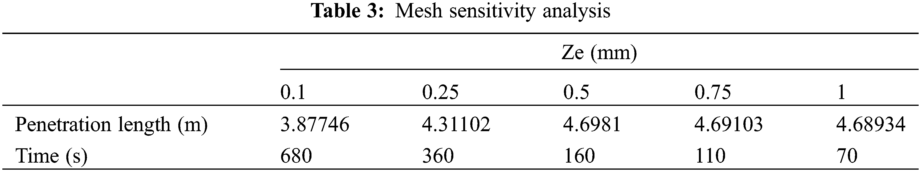
In this numerical model, the water-to-cement ratio (W/C), viscosity, and initial fracture aperture are set as constant of 0.5, 0.432 Pa⋅s, and 0.15 mm, respectively. Furthermore, the initial grouting pressure remains 2 MPa. The mesh size is represented with Ze (zone generate edge-length). Five levels of Ze are employed in the numerical model, including 0.1, 0.25, 0.5, 0.75, and 1 mm.

Table 3 presents the final grouted penetration length and computing time corresponding to each mesh size level. As depicted in Table 3, it is evident that as Ze decreases, the time consume increases gradually while the grouting length decreases. When Ze exceeds 0.5, the penetration length almost keeps constant. Specifically, as Ze decreases from 0.5 to 0.25 mm, the penetration length decreases from 4.69 to 4.31 m. These results indicated that grouting penetration length remains constant as Ze decreases in range of larger than 0.5 mm. Consequently, the threshold for mesh size in this model was finally determined as 0.5 mm to ensure a balance between simulation efficiency and accuracy and the mesh size of following numerical models are set as 0.5 mm.

5.2 Model Verification

In order to evaluate the accuracy of the model algorithm, a single fracture numerical model was established based on the UDEC numerical simulation and used to analyze the variations in grout penetration length and pressure with penetration length. The results were then compared with theoretical outcomes. As shown in Fig. 9, the plane model was 10 m long and 5 m high, having a grouting hole diameter of 0.1 m, an initial crack width of 0.015 mm, and considered the crack width opening. The basic parameters of the model are presented in Table 2. The basic parameters of the slurry were chosen based on those with a W/C ratio of 0.5.

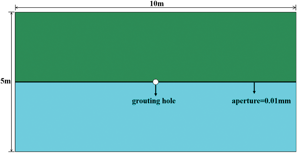
Figure 9: Algorithm validation model

By incorporating the time-varying algorithm into the UDEC model, grouting simulations are conducted at a constant pressure of 2 MPa in the grouting hole. The simulation results are compared with the theoretical results calculated using formulas (3)–(28), as depicted in Fig. 10. Under stable grouting pressure, the theoretical solutions and numerical simulation results of grouting penetration length and pressure change show good agreement, with the maximum error not exceeding 5%.

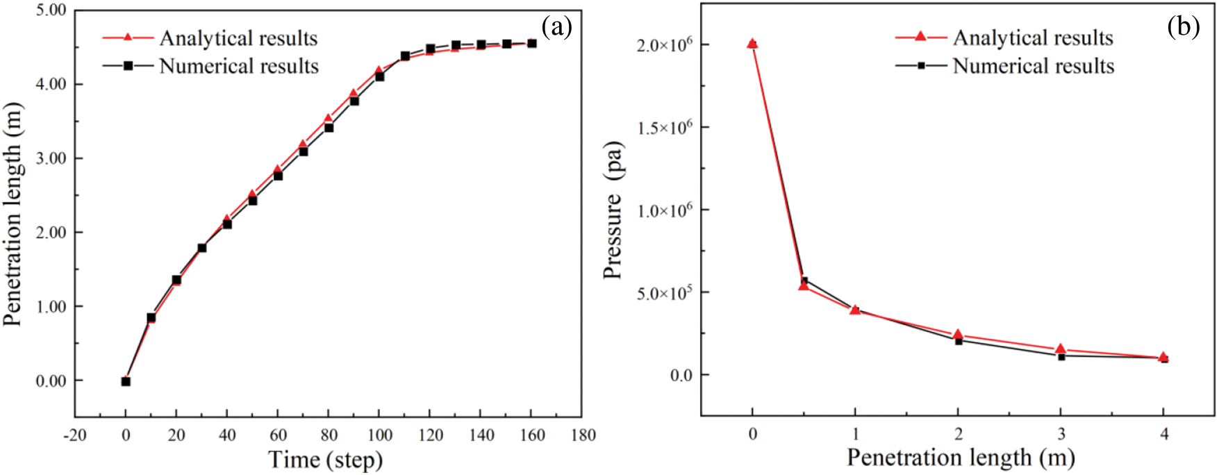
Figure 10: Comparison of the theoretical solution with the numerical solution: (a) The relationship between penetration length and time; (b) pressure distribution in the penetration area

It was assumed in the simulation that the rock surrounding the crack is rigid, signifying that the aperture width does not change when grouting pressure is applied and the slurry flows within the crack. However, rock lithology is not rigid in actual projects and can vary. Under the influence of grouting pressure, the aperture width should be allowed to expand. Neglecting the fracture width change can significantly impact the grouting effect, as only fluid mechanics coupling analysis can accurately simulate this complex process.

Nonetheless, taking advantage of the UDEC numerical simulation software, this process can be effectively simulated, allowing for the definition of both the initial pore size and the final residual pore size under zero normal stress.

According to Rice [42], the fracture aperture under uniform pressure can be expressed as Eq. (31).

a=a0+4p(1−υ2)El2−l02 (31)

where a0 is the initial aperture; l is half of the total length of the fracture; l0 is the distance from the point to the grouting point. In the UDEC numerical model, Young’s modulus E and Poisson’s ratio υ were calculated by E=9KG3K+G and υ=3K−2G(3K+G) ( K and G are bulk modulus and shear modulus, respectively).

The fracture width variation cloud map under uniform pressure was obtained, as shown in Fig. 11. Based on Eq. (31), the fracture width variation trend for each particle in a single fracture was given. A comparison between the theoretical and numerical solutions revealed that they were generally consistent (Fig. 12a), validating the feasibility of using UDEC to simulate the aperture width evolution law. The simulation results of the model with varying aperture widths are shown in Fig. 12b.

Figure 11: Aperture width distribution cloud map

Figure 12: Aperture simulation: (a) Aperture width variation theory and numerical solution; (b) relationship between penetration length and aperture width

In the single crack grouting model, the change in grout penetration length and aperture width was positively correlated when a  < 0.05 mm. The influence of the increase in aperture width on the change in grout penetration length became negligible for a > 0.05 mm. During the grouting pressure process, the maximum aperture width appeared at the position of the grouting hole, and the minimum aperture width appeared at the tip of the grout penetration length. The distance between these two points corresponded to the penetration length of the grouting, indicating that UDEC could effectively simulate the evolution law of aperture width. Simultaneously, the validity of the fluid-solid coupling model of viscosity time-varying grouting diffusion based on UDEC was corroborated.

6  Fracture Grouting Simulation

Based on the theoretical analysis, the impact of grouting diffusion distance was determined using a three-dimensional approach by considering the time-varying viscosity of the HGM slurry with varying W/C ratios and the change in aperture width. The grouting plane model based on UDEC is shown in Fig. 13. The fractures of the rock strata were simulated using interconnected joints, with the grouting holes positioned at the center of the fracture distribution. The dimensions of the three models were 5 m × 10 m, and their primary difference lay in the various forms of fractures. In order to ensure the accuracy of the simulated grouting test, boundary conditions were applied around the model to fix the boundary.

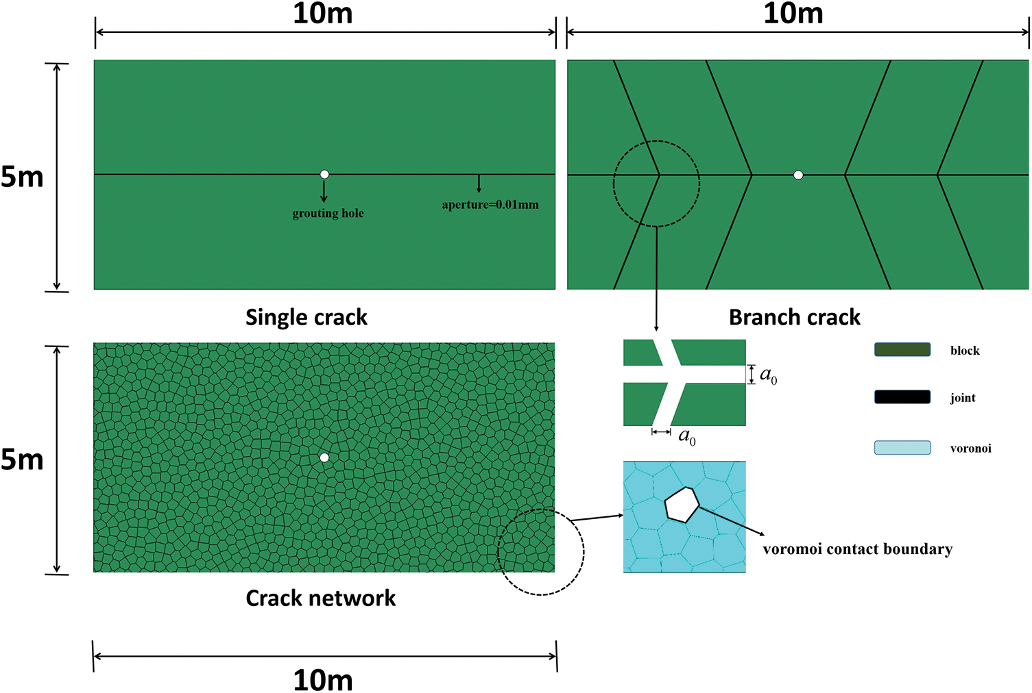
Figure 13: Different grouting plane models

In the fracture network model, the size of the Voronoi was set to 1 mm, generating a total of 1,294 irregular Voronoi. The mesh size was set to 0.5 mm, resulting in 950,317 networks, and the gravitational acceleration was taken as g = 9.8. An independent unit code was utilized to simulate the slurry flow through the joint surface during the grouting process. It was assumed that the slurry flows only inside the fracture, while the blocks around the model are impermeable. The designed value of grouting pressure was 2 MPa, and the grouting stop time was controlled by the number of time steps. The fluid flow algorithm selected was the steady-state flow algorithm.

6.1 Single Fracture

The penetration length, measured as the distance traveled by the grouting material within the fracture, is shown in Fig. 14 for time-varying grouting with different W/C ratios. Overall, the penetration length tended to increase over time for all W/C. As the W/C increased, the slurry had better fluidity, resulting in a farther penetration length in the aperture. However, the HGM slurry with W/C = 0.5 began to flow slowly at t = 80 s, whereas the W/C = 0.4 and W/C = 0.3 slurries flowed slowly at t = 60 s and t = 80 s, respectively. The HGM slurry with W/C = 0.5 had better fluidity overall, as indicated by the higher flow output at the grouting hole in Fig. 15, and achieved a higher filling ratio in the fracture. The final penetration length of the slurry with W/C = 0.5 was 4.69 m, i.e., 0.3 and 0.47 m longer than that observed for slurries with W/C = 0.4 and W/C = 0.3, respectively. Therefore, it was obvious that the HGM slurry with a high W/C had better fluidity during fracture grouting and was closer to the engineering requirements under the same fracture form. Subsequently, further experimentation was conducted on the HGM slurry with W/C = 0.5 to investigate its behavior during fracture grouting.

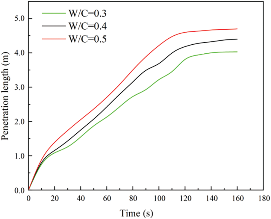
Figure 14: Relationship between penetration length and time at different W/C ratios

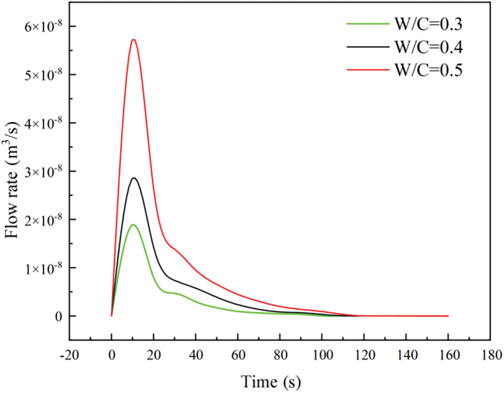
Figure 15: Relationship between flow and time at grouting holes with different W/C ratios

Based on the UDEC viscosity time-varying model, the grout penetration length at different times is shown in Fig. 16. The slurry diffused from the center of the grouting hole to the left and right sides, and the pressure also decreased from the grouting hole towards both sides. Since the slurry only flowed within the fracture, the pressure displayed here represented the pressure inside the aperture. The following three different conditions were considered for simulation:

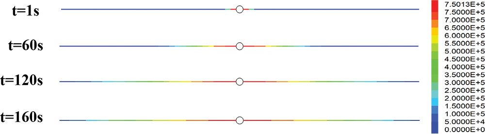
Figure 16: Viscosity time-varying model for grout penetration length at different times

Test 1: constant aperture width and constant viscosity.

Test 2: changing aperture width and constant viscosity.

Test 3: variation of aperture width and viscosity.

The relationship between penetration length and time is shown in Fig. 17a, and the final grout penetration length of the HGM slurry under different conditions varies. Comparing Test 1 and Test 2, the penetration length increased at each grouting time with the increasing grouting time, with the total increase being 0.244 m at t = 160 s. For Test 2 and Test 3, the penetration length was about the same before t = 60 s. After t = 60 s, the growth rate of penetration length in Test 3 was affected by the increase in the viscosity of the HGM slurry value. Before reaching 120 s, the actual penetration length in Test 3 was 1.14% lower than in Test 2. When t = 120 s, the circulation command ran for the second time, and the value of the slurry’s viscosity changed again. After reaching 160 s, the grouting stopped, which was 1.08% lower than the previous cycle. Finally, considering the time-varying viscosity of the slurry, the penetration length was 0.124 m lower than that of the constant viscosity.

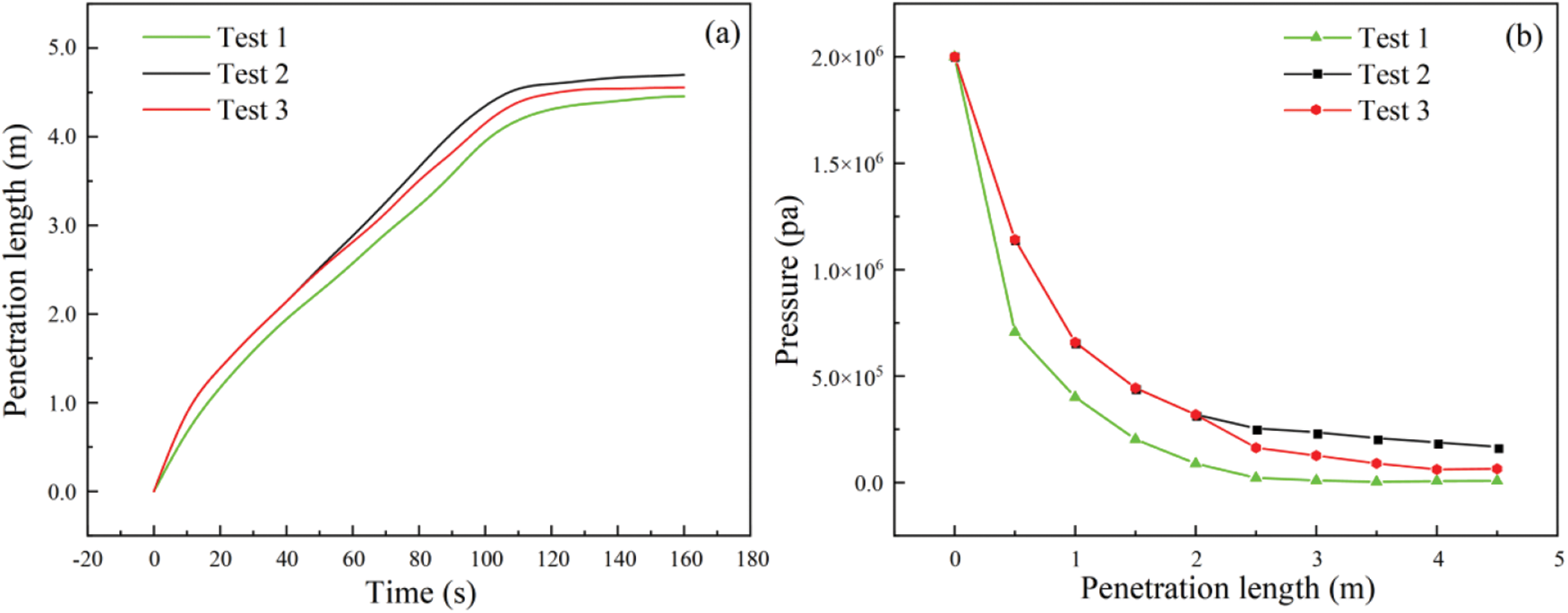
Figure 17: Single fracture grouting simulation results: (a) The relationship between penetration length and time under different conditions; (b) pressure distribution with penetration length under different conditions

The pressure distribution in the penetration length region is shown in Fig. 17b. When t  < 60 s, Test 2 and Test 3 showed the same pressure distribution at the same penetration length, as the time-varying model did not change. In the single fracture grouting model, the increase in aperture width significantly increased for the grout penetration length. The influence of the aperture change on the grout penetration length was 0.12 m higher than that of the slurry time-varying viscosity. Since the single fracture model was relatively simple, further development focused on the branch fracture and fracture network grouting processes.

6.2 Branch Fracture

The calculation model is shown in Fig. 13, whereas the distribution of grouting pressure at different times is shown in Fig. 18. At t = 40 s, the slurry passed through the first bifurcation of the branch fracture under the influence of grouting pressure. The slurry diffused to the three different branches at equal distances. At t = 100 s, the slurry passed through the second bifurcation fracture, and the final calculation steps ended grouting at t = 300 s.

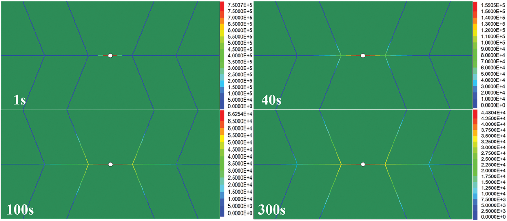
Figure 18: Grouting pressure distribution at different times of the viscosity time-varying model

Fig. 19a shows the penetration length of the fracture grouting under three different conditions. Comparing Test 2 with Test 3, like the single fracture grouting simulation, the penetration lengths of the two were the same before t = 60 s. In Test 3, the length began to grow slowly due to the change in its viscosity relative to Test 2 after t = 60 s. Until the final grouting completion time t = 300 s, the actual penetration length in Test 3 was 0.294 m less than that of Test 2.

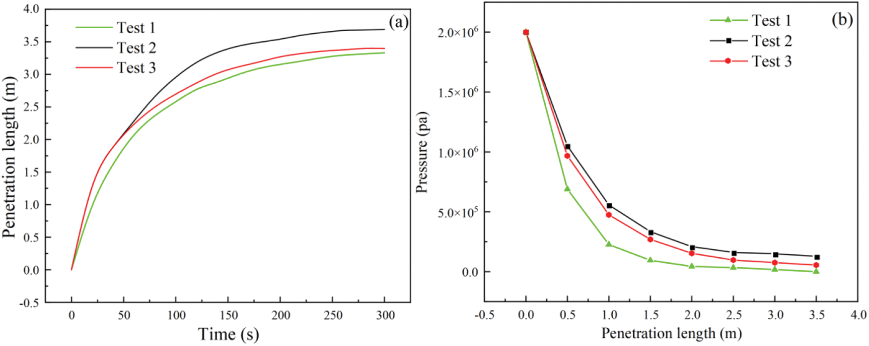
Figure 19: Simulation results of branch cracks: (a) The relationship between penetration length and time under different conditions; (b) pressure distribution with penetration length under different conditions

At the beginning of the grouting pressure application, the penetration length in Test 1 was less than that in Test 2 at each moment. Eventually, the final penetration length in Test 2 gradually approached the value in Test 3. When t = 300 s, the penetration length in Test 1 was 0.360 m less than that in Test 2.

The relation between grout penetration length and pore pressure under three different working conditions is shown in Fig. 19b. Under the same penetration length, the pore pressure of the three conditions at each time was in the order of Test 1 < Test 3 < Test 2. Further, the variation in aperture width during grouting was analyzed. At t = 20 s, the aperture width around the grouting hole increased to 0.171 mm. At t = 100 s, the maximum aperture width at the grouting hole decreased to 0.163 mm. When the final grouting time reached t = 300 s, the maximum aperture width decreased to 0.158 mm. Unlike the single fracture grouting simulation, the maximum width of the aperture did not appear in the position closest to the grouting hole in the branch fracture model.

As shown in Fig. 20, when the slurry flowed from the Joint1 channel to Joint 2, Joint 3, and Joint 4 channels, the increase in the aperture width of the other three channels led to the deformation of the surrounding rock mass due to grouting pressure. As a result, the aperture width of the Joint1 channel near the bifurcation crack continued to increase on the original basis, leading to the aperture section of the Joint1 channel of the crack near the bifurcation crack being larger than that near the grouting hole.

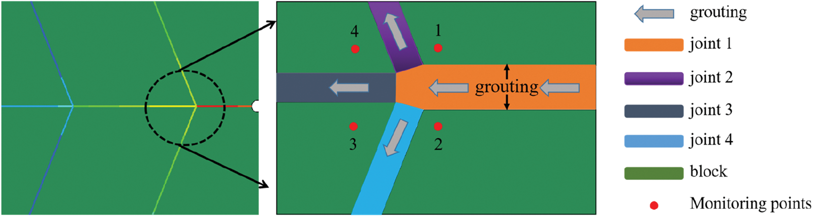
Figure 20: Diagram of aperture width change at the branch bifurcation

As shown in Fig. 21a, the maximum opening of the crack was 0.158 mm at the end of the final calculation, which was 0.3–1 m away from the grouting hole. The crack opening at 0–0.3 m around the grouting hole was only 0.157 mm after the maximum crack opening. The reason for the disparity between the analysis and the single fracture grouting simulation was that the change in the aperture width caused mutual extrusion between the rock masses around the fracture under the action of grouting pressure in the branch fracture model, resulting in a difference between the final result and the single fracture grouting simulation.

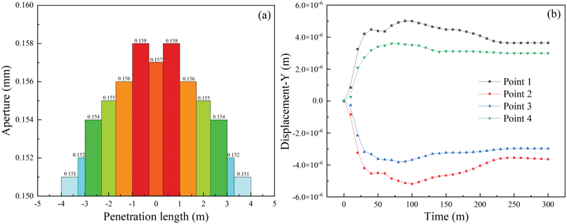
Figure 21: Analysis of aperture variation: (a) The numerical relationship between penetration length and aperture width at t = 300 s; (b) the Y-directional displacement of the monitoring point

In order to elucidate the aforementioned reasons, four Y-direction displacement monitoring points were set at the bifurcation fracture. The results are shown in Fig. 21b, with negative values indicating downward movement along the Y direction. When t = 300 s, the total displacement of rock mass at monitoring points 1 and 2 was 0.008 mm, and when t = 300 s, the crack width at the bifurcation crack increased by y=4.04e−6+|−4.04e−6|=8.08e−6 mm, which corresponded to the displacement value at this point. Similarly, the change in displacement and fracture opening at any point during the numerical fracture grouting simulation could be calculated, corroborating the accuracy of the analysis. This phenomenon is known as fracture-fracture interaction [43].

6.3 Fracture Network

In Sections 6.1 and 6.2, the grouting simulations of single fracture and branch fracture were studied to reflect the complex diversity of fracture interiors in practical engineering. Building on this, a fracture network based on the UDEC numerical model was established. The model randomly generated a fracture network through Voronoi Tyson multi-deformation. The Voronoi grouting flow diagram is shown in Fig. 22. The Tyson polygon boundary represented the fracture network. The fluid flowed only within the fractures and did not penetrate the Voronoi blocks. Under grouting pressure, it flowed along the Tyson polygon boundaries. The basic parameters of the model area are presented in Table 2.

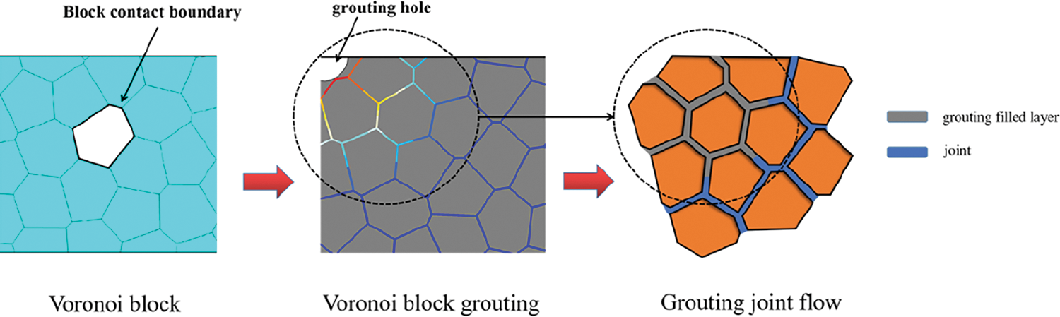
Figure 22: Grouting flow diagram of the fracture network

Fig. 23a shows the variation of grout penetration length with time under three different working conditions. At the grouting completion time of t = 600 s, the penetration lengths in Test 1, Test 2, and Test 3 were found as 1.43, 1.49, and 1.15 m, respectively. In Test 1 and Test 2, the trend of penetration length change transitioned from relative growth to late approximation. This was because the increase in aperture width in the early stage of Test 2 positively impacted the grout penetration length. With the increase in grouting time, the decrease in pore size width hindered the slurry flow to some extent. The influence of aperture width changes on penetration length was 0.06 m. After t = 150 s, the penetration length in Test 1 was larger than that in Test 3, and the influence of viscosity on the penetration length gradually dominated. Comparing Test 2 with Test 3, the effect of viscosity changes on penetration length was 0.35 m at t = 600 s. After pressure was applied to the grouting hole, the pressure at the grouting hole decreased with the increasing grout penetration length. The pressure in the grouting simulation decreased with the increase in penetration length under different conditions, as shown in Fig. 23b. When t < 150 s, the pore pressure for the three tests at each time was in the order of Test 1 < Test 3 < Test 2 under the same penetration length. When t >150 s, the relationship between the three changed to Test 3 < Test 1 < Test 2.

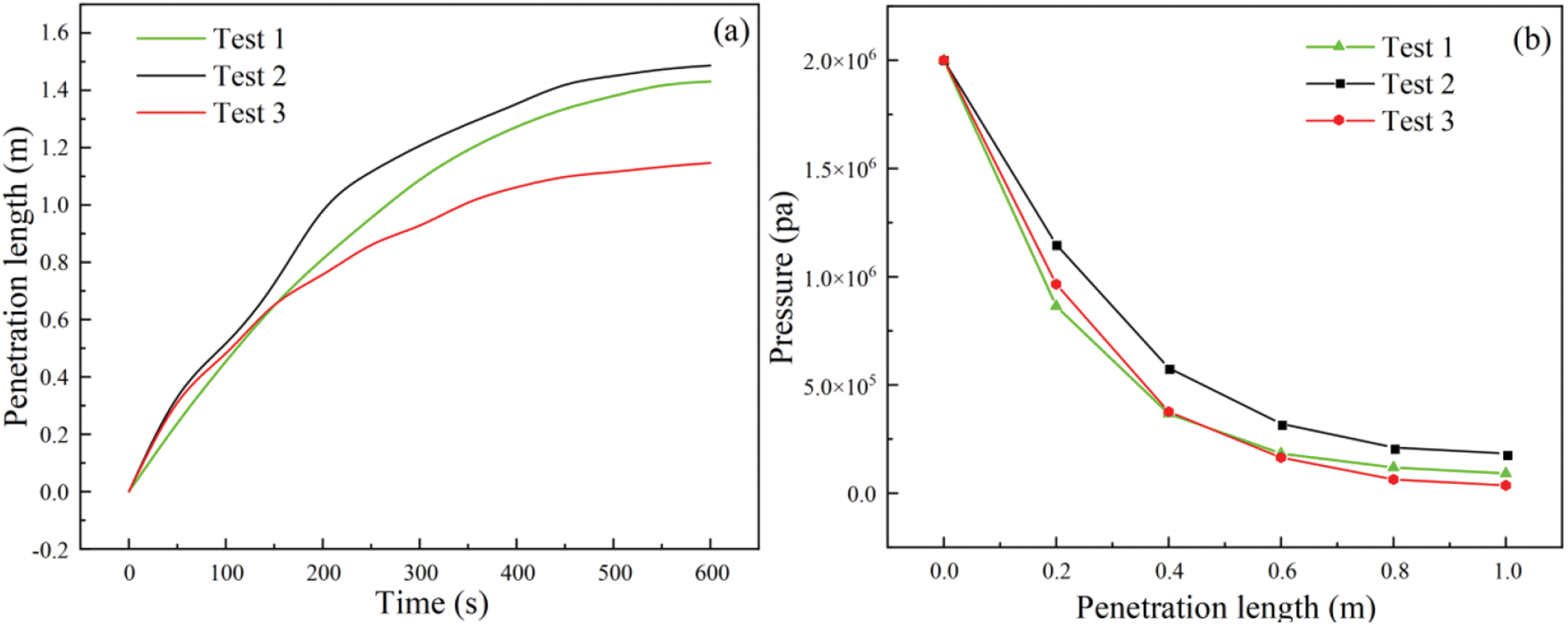
Figure 23: Fracture network simulation results: (a) The relationship between penetration length and time under different conditions; (b) pressure distribution with penetration length under different conditions

The ratio of aperture opening or closing at different grouting times is shown in Fig. 24. It can help study the evolution law of aperture width in the seepage area based on the viscosity time-varying grouting fracture network model, with the initial fracture opening being 0.15 mm. When t = 100 s, under the action of grouting pressure, the increase in fracture opening accounted for 78.1%, and the decrease in fracture opening accounted for 21.9%. The change of fracture opening decreased with the distance from the grouting hole. The maximum fracture opening appeared near the grouting hole at 0.198 mm, and the change of fracture opening in the area far from the grouting hole was stable between 0.15 and 0.16 mm, accounting for 63.2% of the whole area. However, when t = 300 s, the proportion increased to 76.5%. When the final grouting time t = 600 s, it increased to 88.4%. The maximum aperture width was 0.20 mm, the aperture width decreased by 5.4%, and the aperture width increased in the whole penetration area by 94.6%. Based on the evolution law of pore size width in the grouting simulation, the pore area was positively correlated with the grouting time, and the decreased area was negatively correlated. With the increased grouting time, the change of pore size width in the infiltration area tended to stabilize at a value of 0.15–0.16 mm.

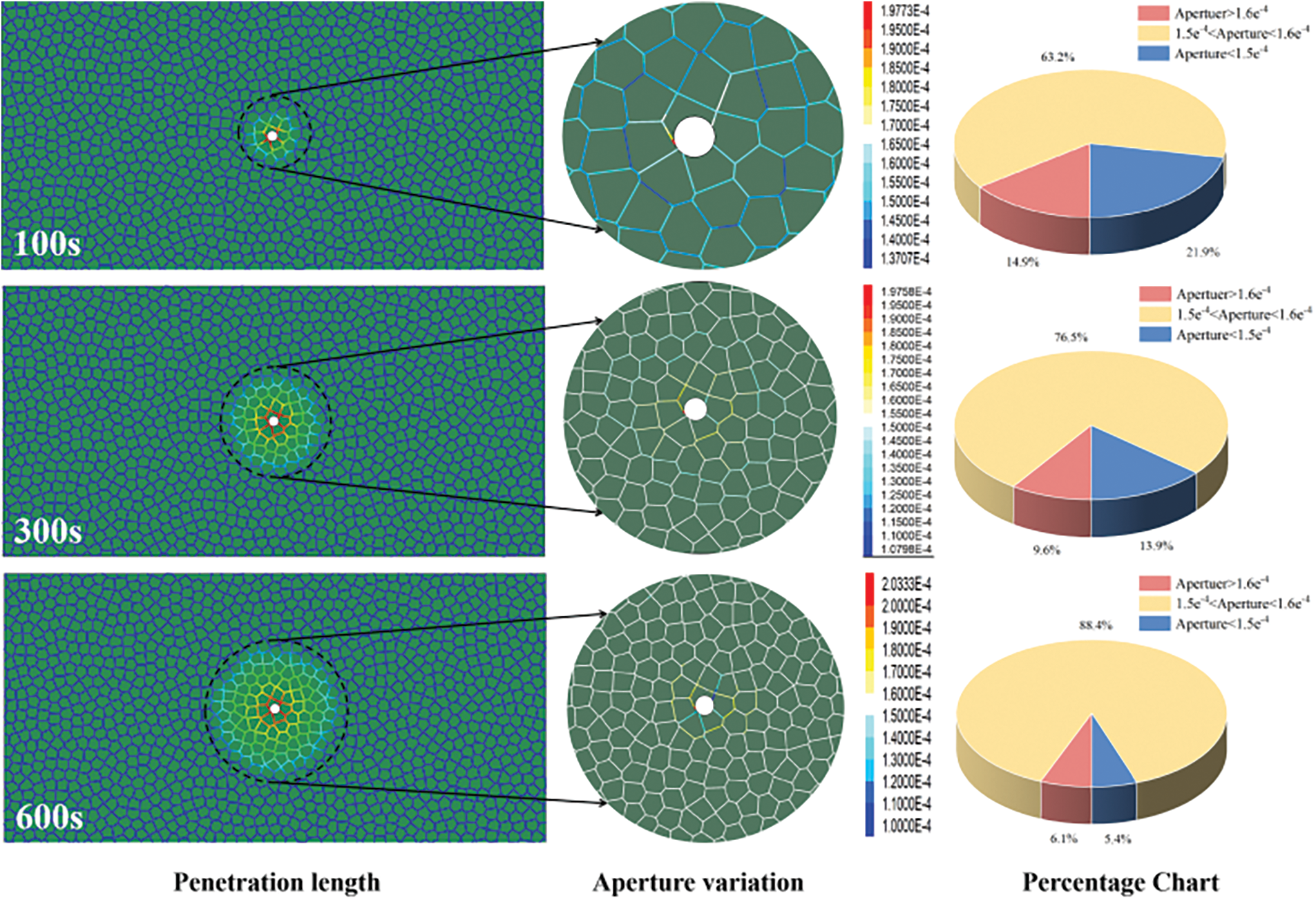
Figure 24: The change of pore width in the penetration length region at different times

Since the final calculation time of previous research did not fully reflect the entire evolution process of the viscosity of HGM cement slurry with time, the initial constant grouting pressure was increased by 10 MPa, the final grouting end time was t = 1800 s, the geometric parameters of the fracture network simulation were 10 m long and 10 m wide, and the radius of the grouting hole was 0.1 m. The basic parameters of the model are presented in Table 2.

Fig. 25a shows the relationship between the penetration length and time at t = 1800 s for constant viscosity and time-varying viscosity of the HGM slurry. As shown in Fig. 4a, the boundary of the viscosity growth hysteresis zone and rapid growth zone was at t = 1200 s. When the grouting time was less than 1200 s in the viscosity growth hysteresis zone, the total penetration length was 3.33 m. However, after the viscosity time-varying HGM slurry entered the rapid viscosity growth zone, the final penetration length of the viscosity time-varying model increased by 3.57 m, which was 1.1 m less than that in the constant viscosity simulation. The pore pressure of the viscosity time-varying model under any grout penetration length was smaller than that of the constant viscosity model under the same penetration length, as shown in Fig. 25b.

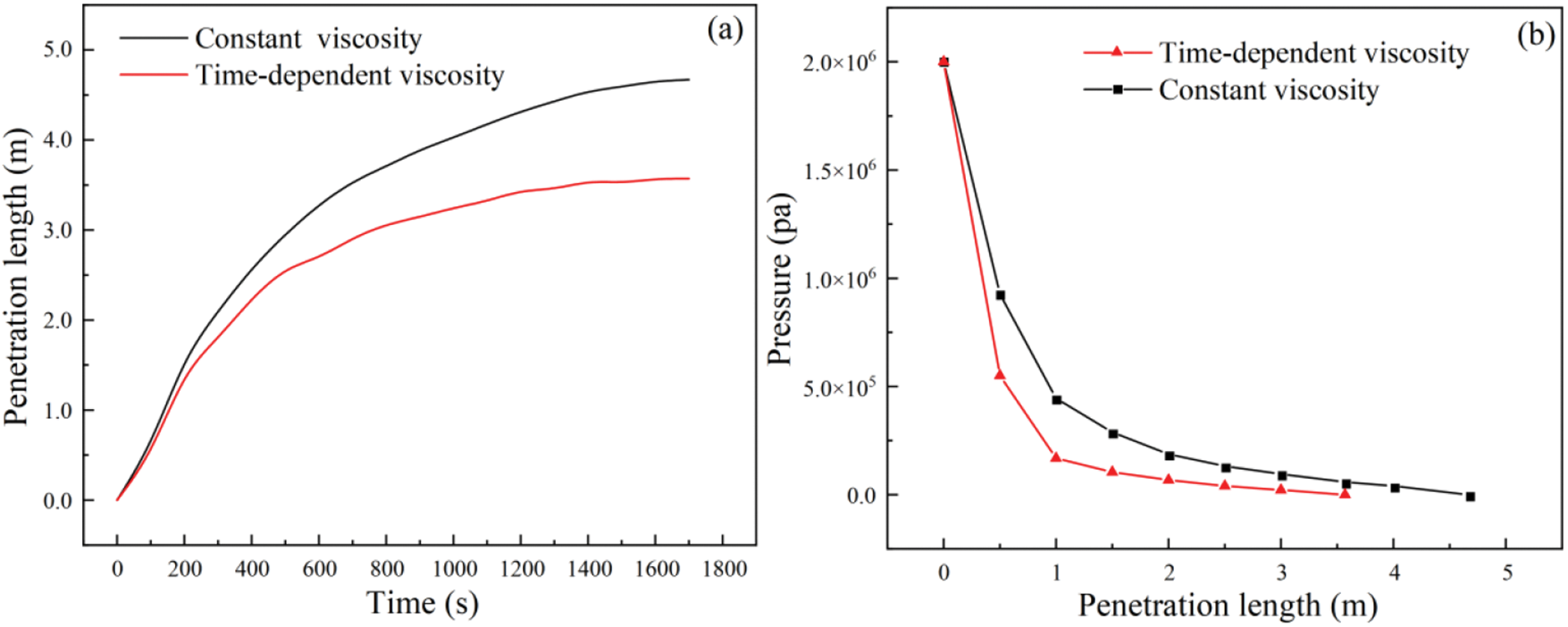
Figure 25: Grouting simulation results after changing the model: (a) The relationship between penetration length and time; (b) pressure distribution in the infiltration area

7  Conclusions

In this study, a fluid-solid coupling model of grouting diffusion with time-varying viscosity was developed based on the discrete element method combined with the Bingham fluid flow equation. The developed model was validated by the theoretical solution. The effects of slurry viscosity time-varying and pore size width variation on grout penetration length were discussed through different fracture forms (single fracture, branch fracture, and fracture network model). The process of viscosity time-varying was simulated by adjusting the model. The following conclusions are drawn from the obtained results.

The viscosity time-varying function obtained by experimentation show that the changing trend of HGM slurry viscosity with time under different W/C ratios is positively correlated. The viscosity growth form is divided into two intervals, i.e., the growth hysteresis and rapid growth zones; the interval boundary is the pumpable slurry period.

Based on the test viscosity time-varying function and Bingham flow equation, combined with the UDEC joint seepage model, the fluid-solid coupling model of viscosity time-varying grouting diffusion was established. The applicability of the model was corroborated by the theoretical solution.

Under different fracture forms, the influence of time-varying viscosity on grout penetration length is different under the same grouting process conditions, manifested in single fracture, 0.124 m; branch cracks, 0.294 m; and fracture network, 0.350 m. In the complex fracture model, the time-varying viscosity greatly influences the penetration length. By adjusting the model and grouting pressure, the whole process of viscosity evolution with time was simulated, and the final penetration length was 1.1 m.

Acknowledgement: The authors sincerely thank the anonymous reviewers for their helpful suggestions.

Funding Statement: This work was supported by the National Natural Science Foundation of China (Grant Numbers: U22A20234, 42277170) and the Key Research and Development Project of Hubei Province (Grant Number: 2020BCB073).

Author Contributions: The authors confirm contribution to the paper as follows: study conception and design: Xuewei Liu, Ying Fan; data collection: Lei Zhu, Wei Deng, Wenjie Yao; analysis and interpretation of results: Lei Zhu, Bin Liu; draft manuscript preparation: Lei Zhu, Xuewei Liu. All authors reviewed the results and approved the final version of the manuscript.

Availability of Data and Materials: The data that support the findings of this study are available from the corresponding author upon reasonable request.

Conflicts of Interest: The authors declare that they have no conflicts of interest to report regarding the present study.

References

1. Martino, J. B., Chandler, N. A. (2004). Excavation-induced damage studies at the underground research laboratory. International Journal of Rock Mechanics and Mining Sciences, 41(8), 1413–1426. [Google Scholar]

2. Seo, H. J., Choi, H., Lee, I. M. (2016). Numerical and experimental investigation of pillar reinforcement with pressurized grouting and pre-stress. Tunnelling and Underground Space Technology, 54, 135–144. [Google Scholar]

3. Hassler, L., Stille, H., Hakansson, U. (1987). Simulation of grouting in jointed rock. 6th International Congress on Rock Mechanics (ISRM)Canada, Montreal. [Google Scholar]

4. Lin, T., Zhao, Z. H. (2021). Block-based dem modeling on grout penetration in fractured rock masses. Chinese Journal of Underground Space and Engineering, 17(4), 1080–1090. [Google Scholar]

5. Wallner, M. (1976). Propagation of sedimentation stable cement pastes in jointed rock. Rock Mechanics and Waterways Construction, 2, 132–136. [Google Scholar]

6. Wereley, N. M., Pang, L. (1998). Nondimensional analysis of semi-active electrorheological and magnetorheological dampers using approximate parallel plate models. Smart Materials and Structures, 7(5), 732. [Google Scholar]

7. Lombardi, G. (1985). The role of cohesion in cement grouting of rock. Proceedings of the 15th International Congress on Large DamSwitzerland, Lausanne. [Google Scholar]

8. Yang, Z. X., Lei, J. S. (2005). Study on grouting diffusion radius of exponential fluids. Rock and Soil Mechanics, 26(11), 1803–1806. [Google Scholar]

9. Yang, X. Z., Wang, X. H., Lei, J. S. (2004). Study on grouting diffusion radius of Bingham fluids. Journal of Hydraulic Engineering, 6, 75–79. [Google Scholar]

10. Yang, Z. Q., Hou, K. P. (2014). Study on the diffusion radius of Bingham fluid in the form of cylindrical seepage grouting. Modern Tunnelling Technology, 51, 103–109. [Google Scholar]

11. Li, S., Liu, R., Zhang, Q. S., Sun, Z. Z., Zhang, X. (2013). Research on CS slurry diffusion mechanism with time-dependent behavior of viscosity. Chinese Journal of Rock Mechanics and Engineering, 32(12), 2415–2421. [Google Scholar]

12. Ruan, W. J. (2005). Spreading model of grouting in rock mass fissures based on time-dependent behavior of viscosity of cement-based grouts. Chinese Journal of Rock Mechanics and Engineering, 24(15), 2709–2714. [Google Scholar]

13. Zhao, Y. L., Luo, S. L., Wang, Y. X., Wang, W. J., Zhang, L. Y. (2017). Numerical analysis of karst water inrush and a criterion for establishing the width of water-resistant rock pillars. Mine Water Environ, 36, 508–519. [Google Scholar]

14. Saada, Z., Canou, J., Dormieux, L. (2006). Evaluation of elementary filtration properties of a cement grout injected in a sand. Canadian Geotechnical Journal, 43(12), 1273–1289. [Google Scholar]

15. Saada, Z., Canou, J., Dormieux, L. (2005). Modeling of cement suspension flow in granular porous media. International Journal for Numerical and Analytical Methods in Geomechanics, 29(7), 691–711. [Google Scholar]

16. Liu, J., Liu, R. T. (2012). Diffusion law model test and numerical simulation of cement fracture grouting. Chinese Journal of Rock Mechanics and Engineering, 31(12), 2445–2452. [Google Scholar]

17. Zhao, Y. L., Liu, Q., Zhang, C. H., Liao, J., Lin, H. (2021). Coupled seepage-damage effect in fractured rock masses: Model development and a case study. International Journal of Rock Mechanics and Mining Sciences, 144, 104822. [Google Scholar]

18. Eriksson, M., Stille, H., Andersson, J. (2000). Numerical calculations for prediction of grout spread with account for filtration and varying aperture. Tunnelling and Underground Space Technology, 15(4), 353–364. [Google Scholar]

19. Chen, T. L., Zhang, L. Y., Zhang, D. L. (2014). An FEM/VOF hybrid formulation for fracture grouting modelling. Computers and Geotechnics, 58, 14–27. [Google Scholar]

20. Xiao, F., Zhao, Z. Y. (2020). Influence of fracture deformation on grout penetrability in fractured rock masses. Tunnelling and Underground Space Technology, 1102, 0886–7798. [Google Scholar]

21. Wang, Q., Feng, Z., Wang, L., Tang, D., Feng, C. (2016). Numerical analysis of grouting radius and grout quantity in fractured rock mass. Journal of China Coal Society, 40(10), 2588–2595. [Google Scholar]

22. Wang, Q. (2018). Grouting reinforcement technical study and engineering application of broken coal-rock massin Lu’an mining district. Beijing, China: Graduate School of China Coal Research Institute. [Google Scholar]

23. Lee, J. S., Bang, C. S., Mok, Y. J., Joh, S. H. (2000). Numerical and experimental analysis of penetration grouting in jointed rock masses. International Journal of Rock Mechanics and Mining Sciences, 37(7), 1027–1037. [Google Scholar]

24. Saeidi, O., Stille, H., Torabi, S. R. (2013). Numerical and analytical analyses of the effects of different joint and grout properties on the rock mass groutability. Tunnelling and Underground Space Technology, 88, 11–25. [Google Scholar]

25. Liu, Q. S., Sun, L. (2019). Simulation of coupled hydro-mechanical interactions during grouting process in fractured media based on the combined finite-discrete element method. Tunnelling and Underground Space Technology, 88, 472–486. [Google Scholar]

26. Mortazavi, A., Maadikhah, A. (2016). An investigation of the effects of important grouting and rock parameters on the grouting process. Geomechanics and Geoengineering, 11(3), 219–235. [Google Scholar]

27. Liu, X. W., Hu, C., Liu, Q. S., He, J. (2021). Grout penetration process simulation and grouting parameters analysis in fractured rock mass using numerical manifold method. Engineering Analysis with Boundary Elements, 123, 93–106. [Google Scholar]

28. Liu, X. W., Chen, H. X., Liu, Q. S., Liu, B. (2022). Modelling slurry flowing and analyzing grouting efficiency under hydro-mechanical coupling using numerical manifold method. Engineering Analysis with Boundary Elements, 134, 66–78. [Google Scholar]

29. Mohajerani, S., Baghbanan, A., Wang, G. (2017). An efficient algorithm for simulating grout propagation in 2D discrete fracture networks. International Journal of Rock Mechanics and Mining Sciences, 98, 67–77. [Google Scholar]

30. Pan, Y. H., Qi, J. R., Zhang, J. F., Peng, Y. X., Chen, C. (2022). A comparative study on steady-state water inflow into a circular underwater tunnel with an excavation damage zone. Water, 14(19), 3154. [Google Scholar]

31. Zhao, J., Fang, Y., Yan, S. Q., Qiu, S. L. (2021). Study on shear mechanical properties of sawtooth structure with different water cement ratios grouting. Chinese Journal of Rock Mechanics and Engineering, 40, 2673–2680. [Google Scholar]

32. Yang, M. J., Yue, Z. Q., Lee, P. K., Su, B., Tham, L. G. (2002). Prediction of grout penetration in fractured rocks by numerical simula. Canadian Geotechnical Journal, 39(6), 1384–1394. [Google Scholar]

33. Lombardi, G. (2003). Grouting of rock masses. International Conference on Grouting and Ground Treatment, 164–197. [Google Scholar]

34. Wang, D. L., Hao, B. Y. (2021). Theoretical and numerical analysis of slurry diffusion with different flow patterns in fracture, vol. 52, no. 10, pp. 3760–3770. China: Central South University Press. [Google Scholar]

35. He, S. D., Li, Y. R., Aydin, A. (2018). A comparative study of UDEC simulations of an unsupported rock tunnel. Tunnelling and Underground Space Technology, 72, 242–249. [Google Scholar]

36. Sinha, S., Abousleiman, R., Walton, G. (2022). Effect of damping mode in laboratory and field-scale universal distinct element code (UDEC) models. Rock Mechanics and Rock Engineering, 55, 2899–2915. [Google Scholar]

37. Barton, N., Bandis, S., Bakhtar, K. (1985). Strength, deformation and conductivity coupling of rock joints. International Journal of Rock Mechanics and Mining Sciences & Geomechanics Abstracts, 22(3), 121–140. [Google Scholar]

38. Itasca Consulting Group Inc. (2014). UDEC (Universal Distinct Element CodeVersion 6.0. Minneapolis: ICG. [Google Scholar]

39. Yang, H. Y. (2016). Rheology of viscosity changes with time grout material and research of diffusion mechanism of grouting in rock mass fissures. Chengdu, China: Chengdu University of Technology. [Google Scholar]

40. Ma, H., Liu, Q. (2017). Prediction of the peak shear strength of sandstone and mudstone joints infilled with high water–cement ratio grouts. Rock Mechanics and Rock Engineering, 50(8), 2021–2037. [Google Scholar]

41. Li, X., Gu, X., Xia, X., Madenci, E., Chen, X. et al. (2022). Effect of water-cement ratio and size on tensile damage in hardened cement paste: Insight from peridynamic simulations. Construction and Building Materials, 356, 129256. [Google Scholar]

42. Rice, J. R. (1968). Mathematical analysis in the mechanics of fracture. In: Fracture: An advanced treatise, vol. 2, pp. 191–311. NY: Academic Press. [Google Scholar]

43. Gothäll, R., Stille, H. (2010). Fracture–fracture interaction during grouting. Tunnelling and Underground Space Technology, 25(3), 199–204. [Google Scholar]