
 Submit a Paper
 Propose a Special lssue
 Open Access
ARTICLE

A New Approach for the Calculation of Slope Failure Probability with Fuzzy Limit-State Functions
1 Department of Engineering Management, Sichuan College of Architectural Technology, Deyang, 61800, China
2 Department of Transport and Municipal Engneering, Sichuan College of Architectural Technology, Deyang, 61800, China
3 Department of Basic Teaching, Sichuan College of Architectural Technology, Deyang, 61800, China
4 Sichuan Hongye Construction Software Co., Ltd., Chengdu, 610081, China
* Corresponding Author: Rangling Cao. Email:
Fluid Dynamics & Materials Processing 2025, 21(1), 141-159. https://doi.org/10.32604/fdmp.2024.054469
Received 29 May 2024; Accepted 06 November 2024; Issue published 24 January 2025
 View Full Text
 Download PDF
Abstract
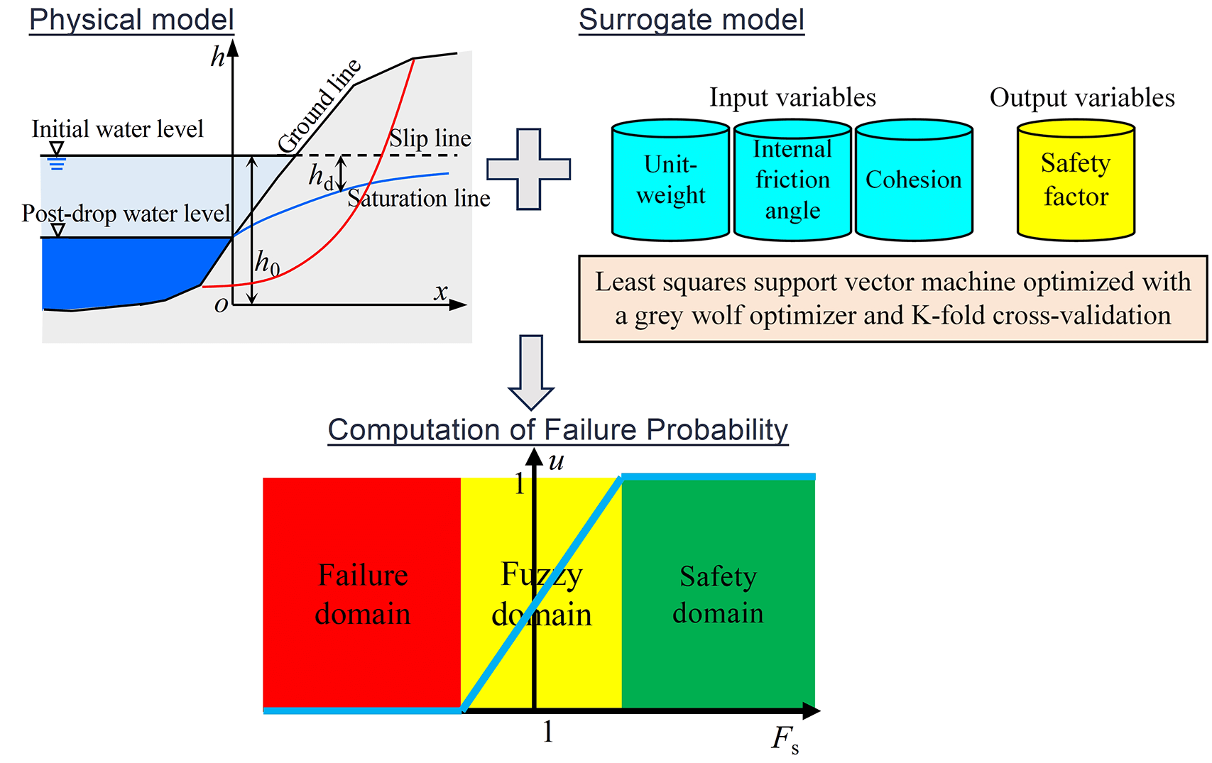
This study presents an innovative approach to calculating the failure probability of slopes by incorporating fuzzy limit-state functions, a method that significantly enhances the accuracy and efficiency of slope stability analysis. Unlike traditional probabilistic techniques, this approach utilizes a least squares support vector machine (LSSVM) optimized with a grey wolf optimizer (GWO) and K-fold cross-validation (CV) to approximate the limit-state function, thus reducing computational complexity. The novelty of this work lies in its application to one-dimensional (1D), two-dimensional (2D), and three-dimensional (3D) slope models, demonstrating its versatility and high precision. The proposed method consistently achieves error margins within 3% of Monte Carlo simulation (MCS) results, while substantially reducing computation time, particularly for 2D and 3D models. This makes the approach highly practical for real-world engineering applications. Furthermore, by applying fuzzy mathematics to handle uncertainties in geotechnical properties, the method offers a more realistic and comprehensive understanding of slope stability. As water is the main factor influencing the stability of slopes, this aspect is investigated by calculating the phreatic line after the change in water level. Relevant examples are used to show that the failure probability of a slope under water wading condition can increase by more than 20% (increase rates in 1D, 2D and 3D conditions being 25%, 27% and 31%, respectively) compared with the natural condition. The influence of diverse fuzzy membership functions—linear, normal, and Cauchy—on failure probability is also considered. This research not only provides a strategy for better calculation of the slope failure probability but also pioneers the integration of computational intelligence, fuzzy logic and fluid-dynamics in geotechnical engineering, presenting an innovative and efficient tool for slope stability analysis.Graphic Abstract
Keywords
Failure probability is a critical metric in the assessment of slope stability, providing essential insights into the potential risk of slope failure [1]. This probability is derived from the inherent uncertainties present in geotechnical mechanical properties, which are primarily influenced by measurement errors and statistical variability.
Currently, probabilistic methods are the primary approach for calculating slope failure probability, largely due to the thorough theoretical development of probabilistic frameworks. These methods are broadly categorized into sampling methods and approximation methods, each with distinct advantages and limitations. MCS is the predominant sampling method employed in this domain. MCS is highly regarded for its accuracy, as it provides a precise probability calculation by simulating numerous possible scenarios. However, a significant drawback of MCS is its computational intensity, especially when dealing with complex limit-state functions [2]. In contrast, approximation methods, such as the first-order first-moment method [3] and the second-order second-moment method [4], offer faster calculations. These methods leverage Taylor series expansions to approximate the failure probability, which significantly reduces computation time. The trade-off, however, is that these methods can incur larger errors when applied to more complex limit-state functions. This discrepancy arises because the approximation may not capture the intricacies of the actual failure mechanisms accurately. To address the computational challenges associated with traditional methods, researchers have explored the integration of computational intelligence technologies. These advanced methods aim to replace or augment complex limit-state functions, thereby reducing computational costs while maintaining accuracy. Notable among these are neural networks [5], which have demonstrated substantial potential in pattern recognition and predictive modeling. Additionally, Kriging techniques [6,7], originally developed for geostatistical applications, have been adapted to estimate failure probabilities by interpolating the outputs of complex models. By leveraging the strengths of these computational intelligence methods, it is possible to achieve a balance between accuracy and computational efficiency. This hybrid approach allows for the effective handling of complex geotechnical data, thereby enhancing the reliability of slope stability analyses.
Fuzzy theory has also been utilized in the computation of failure probabilities for slopes and landslides. These approaches employ fuzzy sets to depict uncertain parameters, facilitating a more supple manifestation of the inherent variability in geotechnical properties [8–12]. Through the employment of fuzzy operations, failure probabilities of slopes can be estimated from a distinct perspective in contrast to traditional probabilistic methods. The considerable advantage of fuzzy sets over probabilistic theory resides in their capacity to capture the distribution of uncertain parameters more effectively, offering a more detailed comprehension of the variability and risks involved [13–15]. Nevertheless, there are prominent challenges related to the application of fuzzy sets in this context. A significant issue is the computational intricacy introduced by fuzzy arithmetic operations. A critical study conducted by Sotoudeh-Anvari [16] highlights that “current fuzzy mathematics is not even in a position to tackle reliably the simplest equations and consequently.” This statement underscores the difficulties faced when performing basic arithmetic operations with fuzzy sets. While addition and subtraction are generally handled with sufficient accuracy, multiplication and division remain controversial and prone to significant errors. These technical challenges necessitate a cautious approach when employing fuzzy sets for slope failure probability estimation. It is essential to recognize the limitations and potential inaccuracies that can arise from the use of fuzzy arithmetic.
In addition to the inherent uncertainty of geological properties, the limit state function itself exhibits a degree of “uncertainty.” Traditionally, many methods have strictly separated the safety and unsafety regions with a critical value of 1, designating areas with a safety factor greater than 1 as safe and those with a factor of 1 or less as unsafe. However, this binary classification does not align with engineering practice, where the reality is often more nuanced. In practice, a slope may remain stable even when the safety factor is slightly above 1, and conversely, it may fail when the safety factor is equal to or less than 1 [17]. This discrepancy highlights the existence of an intermediate state between the safety and unsafety regions, known as the “fuzzy area.” The fuzzy area represents a zone where the slope has a certain possibility of instability, acknowledging the gradation of risk rather than a strict threshold (Fig. 1). Incorporating this ambiguity into the limit state function provides a more realistic and practical assessment of slope stability, reflecting the true nature of geotechnical uncertainties. Considering the ambiguity of the limit state function not only aligns the analysis closer to real-world conditions but also helps avoid the confusing calculations often associated with the concentration of ambiguity in fuzzy sets. This approach allows for a more nuanced and accurate representation of slope stability, recognizing that safety and failure are not always absolute states but exist on a spectrum influenced by various factors. To address these complexities, advanced methods that incorporate fuzzy logic and other computational techniques are necessary. These methods can effectively capture the intermediate state and provide a more comprehensive understanding of the slope’s stability profile. By acknowledging and integrating the fuzzy area, engineers and researchers can develop more robust models that better predict the behavior of slopes under various conditions, ultimately leading to safer and more reliable geotechnical designs.

Figure 1: Definition of safety domain and failure domain: (a) without considering the fuzzification of limit-state function, and (b) considering limit-state function’s fuzzification
The primary contribution of this article is the development of a novel method for calculating failure probability that incorporates the ambiguity of the limit-state function. Traditional methods often struggle with the binary classification of slope stability, which fails to capture the nuanced nature of geotechnical uncertainties. To address this, we propose a method that leverages a LSSVM [18], optimized by the GWO [19] and validated using the K-fold cross-validation technique [20]. This approach aims to provide a more flexible and accurate estimation of failure probabilities by integrating the inherent ambiguities within the limit-state function. The proposed algorithm stands out due to its universal applicability across various slope stability scenarios. By combining LSSVM with GWO, we enhance the optimization process, ensuring that the model parameters are fine-tuned for the best possible performance. The use of K-fold cross-validation further strengthens the model’s reliability by systematically evaluating its predictive capability across multiple subsets of the data. To demonstrate the efficacy and robustness of our method, we conducted comprehensive analyses on one-dimensional (1D), two-dimensional (2D), and three-dimensional (3D) slope models [21].
The rest of this paper is organized as follows. In Section 2, a new calculation method of failure probability is derived and the detailed calculation flow is given. In Section 3, the proposed method is applied to three practical examples, and compared with MCS, which is the most accurate method for calculating the failure probability, the influence of water on slope stability is also investigated, and the influence of the membership function on the results is also discussed. The end is the conclusion drawn by this study.
2.1 Failure Probabilities Calculation Involving Limit-State Function’s Ambiguity
A limit-state function (F) for side-slope stability analysis was often written as [5]:
In the above equation, Fs represents the slope safety factor, which can be calculated using methods including limit equilibrium theory. When F > 0, slopes are considered to be in a safe domain; when F ≤ 0, slopes are considered to be in failed domain. There are many factors affecting the safety factor of slope. Besides the mechanical properties of slope soil, water is also an important factor [22–25].
It can be seen from the definition of Eq. (1) that Fs = 1 is the strict boundary between slope safety domain and failure domain. However, in practice, when the slope Fs is less than 1, it also may not be unstability, and when it is greater than 1, the slope may not be safe. This shows that there is also an intermediate region between the safety and unsafety regions of slopes, which can be both unstability and safe. That is, limit-state functions for slopes are fuzzy, which can be characterized by a fuzzy membership function [26]. Combining fuzzy membership theory, the fuzzy membership for the limit-state function for slope stability is:
In Eq. (2), a and b represent two parameters. In this paper, we set b = 0.5, a = −0.5. That is, if slope Fs is larger than 1.5, one can determine that this slope is in a safe state, and when the slope safety factor is less than 0.5, the slope is considered to be unstable. Slopes with a safety factor between 0.5 and 1.5 are likely to be unstable, and the probability of instability decreases as the slope safety factor increases [17]. According to the form of Eq. (2), Eq. (1) can be rewritten as:
Fig. 2 shows the comparison of Eqs. (2) and (3). Failure probability (Pf) could obtained according to Eq. (4):

Figure 2: Calculation of membership: (a) without considering the fuzzification of the limit-state, and (b) considering the fuzzification of limit-state function
In the equation, N is the number of sampling points. By substituting Eq. (2) into Eq. (4), a failure probability considering limit-state function ambiguity can be calculated, and by substituting Eq. (3) into Eq. (4), a failure probability without considering limit-state ambiguity can be obtained. It can be seen from Eqs. (2) and (3) that when a = b = 0, the method of considering limit-state ambiguity will degenerate into the method of not considering limit-state ambiguity.
The steps for calculating the slope Pf according to the Monte Carlo method are:
1) Sampling, with a total number of N;
2) Calculate u according to Eq. (2);
3) Calculate the failure probability according to Eq. (3).
When Fs expressed by a simple explicit function, Pf can be calculated directly based on the MCS method. When Fs needs to be calculated by a complex implicit iterative procedure, it is extremely time-consuming to directly calculate the failure probability according to the above method. In view of this, a new model is designed below to replace the limit-state function.
2.2 Alternative Model for Limit-States
An LSSVM optimized by the GWO and K-fold CV algorithm is implemented to replace a limit-state function.
GWO, as a new swarm-intelligence algorithm, simulates the hunting process of grey wolves [19]. In this section, we briefly introduce the basic process of GWO.
In GWO, all wolves are divided into four categories (alpha wolves, beta wolves, delta wolves, and omega wolves), and the first three categories guide the behavior of the last one. The process of wolves surrounding the prey is described as follows [19]:
where Xt+1 represents a location of a wolf at (t+1)th iteration, and Xt represents a wolf’s location at tth iteration, and Xp,t represents the prey’s location at tth iteration. During the iteration, b linearly reduces from 2 to 0 [19]. The grey wolves hunting process is modeled as follows:
In the equation, Xα, Xβ, and Xδ are respectively the best guide, second-best guide, and third-best guide. Eqs. (5)–(12) constitute the core of GWO. Unlike the Particle Swarm Optimization [27], which requires the user to specify multiple parameters, there are only two parameters that need to be specified by the user in GWO, i.e., population size and the total iterations.
SVM transforms vectors in an input space to a new feature space using a nonlinear rule, and then converts the actual problem into a quadratic programming problem with inequality constraints. LSSVM is an extension of SVM. LSSVM replaces the inequality constraints in SVM with equality constraints and adopts a squared-error loss function as the training set’s empirical loss, thereby transforming the primary problem into a linear matrix solution problem [18].
The model expression of LSSVM is:
in which, x represents input matrix, wand b are parameters, φ is a nonlinear function.
The parameter w in Eq. (13) is:
in which, λi is Lagrange multiplier, m is sample total number.
According to Eqs. (14) and (13), we have:
and Eq. (15) can also be written as:
In which, K is a kernel function. This paper chooses a gaussian function, defined as follows:
λi and b need to be obtained througth a linear equation:
where
σ in Eq. (17) and C in Eq. (18) are hyperparameters. They can be solved by GWO. The objective function (fitness) of GWO is set to:
Eq. (19) is also called root mean square error (RMSE) function.
When hyperparameters are determined, a K-fold CV algorithm is also performed to divide samples (in Section 3 of this article, K = 5), which is a training method to improve generalization abilityof machine learning.
To better explain the proposed method, Fig. 3 gives a flowchart of calculation method of failure probability proposed in this paper. The following will use 3 examples to verify our method.

Figure 3: Calculation flow chart of the proposed method
It is noted that water is the main factor influencing the stability of slopes. Thus, in the calculation of the safety factor in Eqs. (1)–(4), the effect of water should be incorporated. In this paper, the impact of water on slopes is analyzed through fluid dynamics. Specifically, it is reflected by calculating the phreatic line after the change in water level. Fig. 4 presents a simple model for calculating the saturation line, where h0 represents the initial water level and hd represents the variation of the saturation line.

Figure 4: A simplified model for calculating the saturation line
The differential equation that describes the non-stable motion of diving can be expressed as follows [5]:
where x and t denote the position and time of the calculation point, respectively; a is a coefficient related to the coefficient of permeability. The solution of Eq. (20) can be deduced by Laplace transform, namely:
v0 indicates the rate of water level drop, while M is a sign function, that is:
Based on Fig. 4, the coordinate h of the saturation line can be represented as:
Based on Eqs. (20)–(23), the phreatic line can be determined. Once the phreatic line is determined, the unit weight of the soil above the line is taken as the natural unit weight, and the unit weight below the line is taken as the saturated unit weight.
It is worth noting that all the following calculations are done by MATLAB 2018a on a computer with a Windows 10 system. Fig. 5 shows the iteration curves of the Grey Wolf Optimizer (GWO) for three different slope stability analysis cases (1D, 2D, and 3D slopes). The x-axis represents the number of iterations, and the y-axis indicates the fitness value. Each subfigure (a), (b), and (c) corresponds to Case 1 (1D slope), Case 2 (2D slope), and Case 3 (3D slope), respectively. Fig. 5a depicts the convergence of GWO for the 1D slope is achieved within approximately 20 iterations, indicating efficient optimization. Fig. 5b depicts the iteration curve for the 2D slope, showing similar convergence behavior, reaching the optimum around the 20th iteration. Fig. 5c depicts the iteration curve for the 3D slope, with convergence occurring around the 30th iteration, reflecting the increased complexity of the model.

Figure 5: Iteration curve of GWO: (a) Case one, (b) Case two, (c) Case three
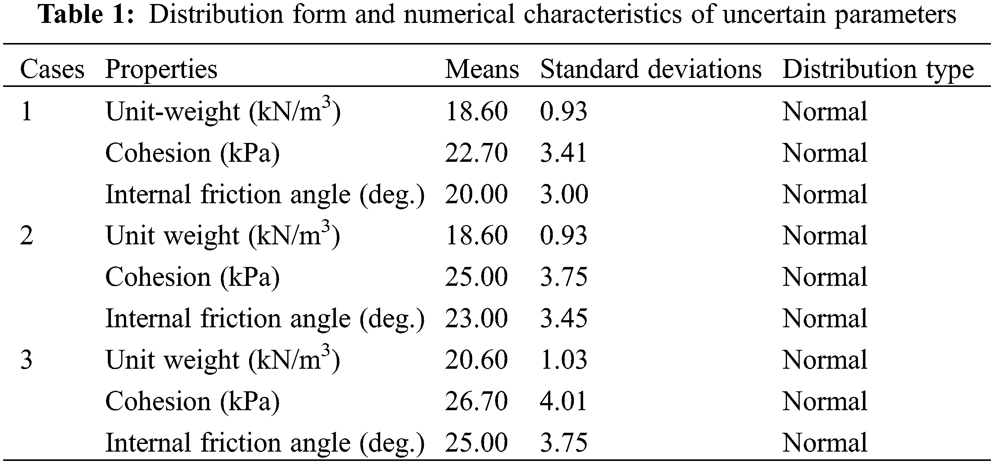
Case 1 is a 1D slope (Fig. 6). On the 1D slope, the slip surface is a straight line. The slope gradient is 30°.The soil’s weight, cohesion, and friction coefficient are uncertain parameters that satisfy the normal distribution (Table 1). The safety factor Fs of the 1D slope is calculated using the following equation:
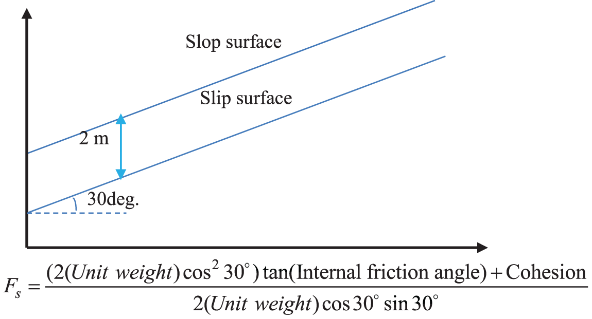
Figure 6: One-dimensional slope
One hundred samples are generated, and the values of C and σ are obtained according to the method in Fig. 3, as shown in Table 2. Among them, the population size and total iterations of GWO are set to 20 and 100, respectively. Fig. 5a shows the iteration curve of GWO. It can be seen that after about 20 generations, GWO tends toward the global optimal value. By setting the sampling times to 30,000, the Pf for this slope is find to be 0.072%. MCS is the most accurate method to calculate the failure probability of landslide. By MCS method, Pf is 0.074%, and the relative deviation between the two is only 2.34%.
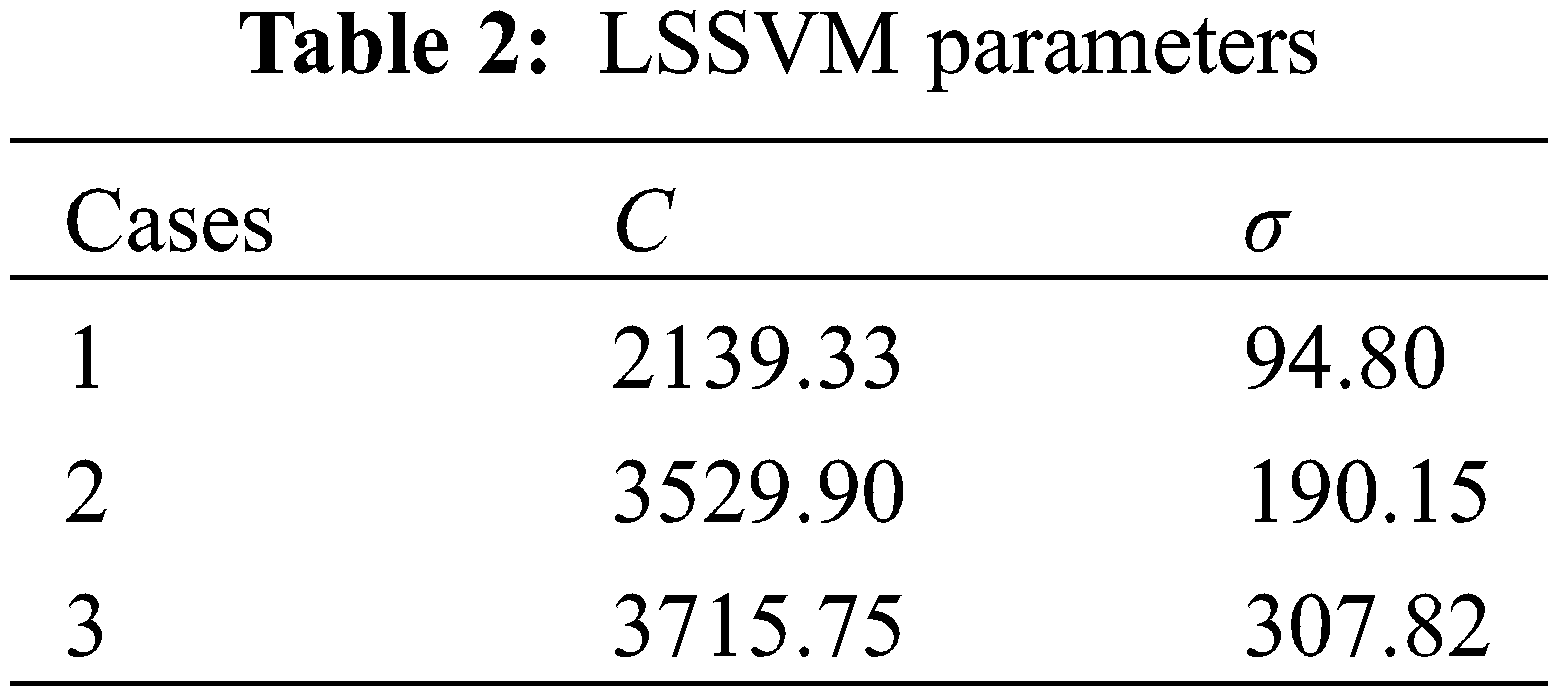
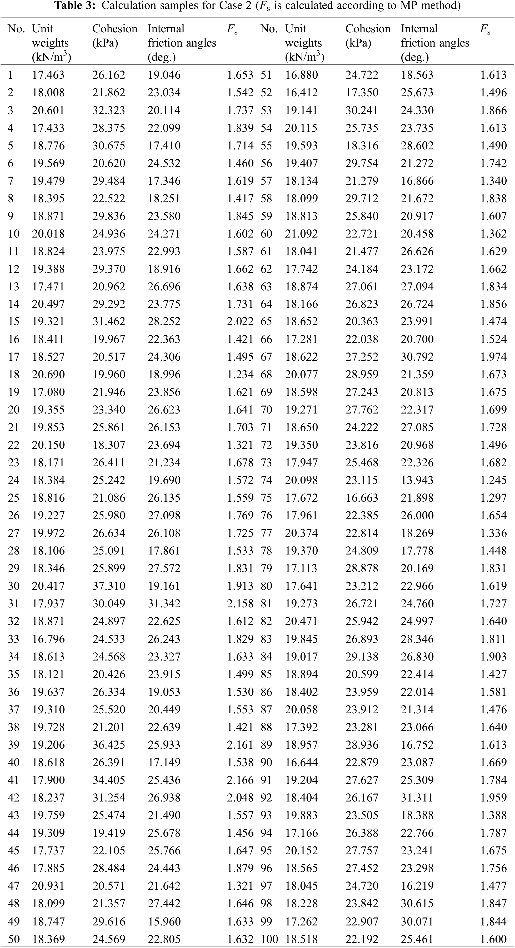
Case 2 is a 2D slope (Fig. 7). On the 2D slope, the slip surface is a curve. In this example, there are three types of normal distributions: the first one is for severity with a mean of 18.60 and a standard deviation of 0.93; the second one is for cohesion with a mean of 25.00 and a standard deviation of 3.75; the third one is for friction angle with a mean of 23.00 and a standard deviation of 3.45. The safety factor for this slope was calculated using the MP method [28]. One hundred samples are generated (Table 3), and the values of C and σ are obtained according to the method in Fig. 3 as shown in Table 2. Fig. 5b shows the iteration curve of GWO. It can be seen that after about 20 generations, GWO tends toward the global optimal value. By setting the sampling times to 30,000 times, a Pf of 2.518% can be obtained. The Pf obtained by MCS method is 2.58%, and the relative deviation between the two is only 2.48%.

Figure 7: Two-dimensional slope
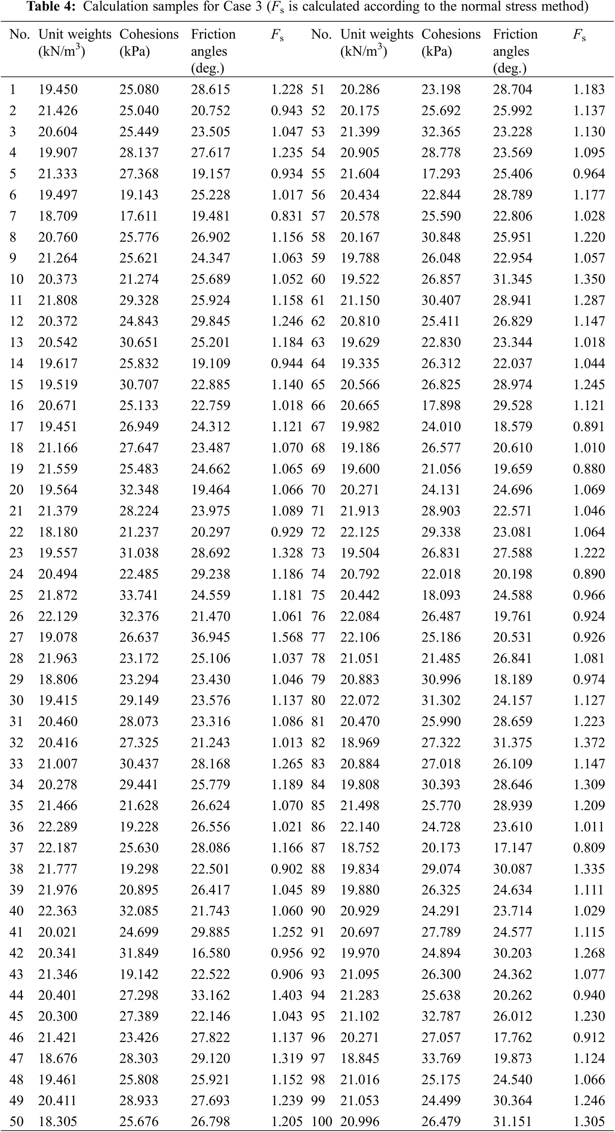
Case 3 is a 3D slope (Fig. 8). In the 3D slope, the slip surface is a curved surface. The slope gradient is 45°. Fig. 8 provides a schematic of a three-dimensional slope used in the case study. This figure illustrates the complex geometry of the 3D slope, including the weight stress and normal stress acting on the slope. In this example, the severity has a mean of 20.60 and a standard deviation of 1.03, the cohesion has a mean of 26.70 and a standard deviation of 4.01, and the internal friction angle has a mean of 25.00 and a standard deviation of 3.75. The safety factor Fs of a 3D slope was calculated using a direct stress [29] approach. As shown in Fig. 8, the method makes it possible for us to obtain Fs by solving the Eq. and adjusting the self-weight stress. The samples used to train the LSSVM are shown in Table 4. Similar to the above two examples, the values of C and σ are 3715.75 and 307.82, respectively. GWO also toward the global optimal solution after 10 iterations. By setting the sampling times to 30,000, the failure probability of this slope is found to be 38.320%. The Pf obtained by MCS method is 37.8%, and the relative deviation between the two is 1.35%.
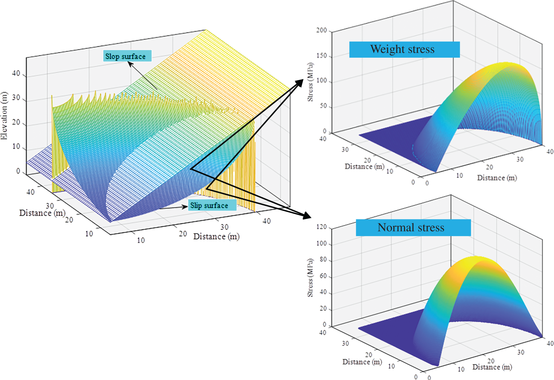
Figure 8: Three-dimensional slope
Water constitutes one of the crucial factors influencing slope stability. Consequently, the proposed methodology is employed to analyze the failure probability of the three slopes under water-immersed conditions (refer to Eqs. (20)–(23)).
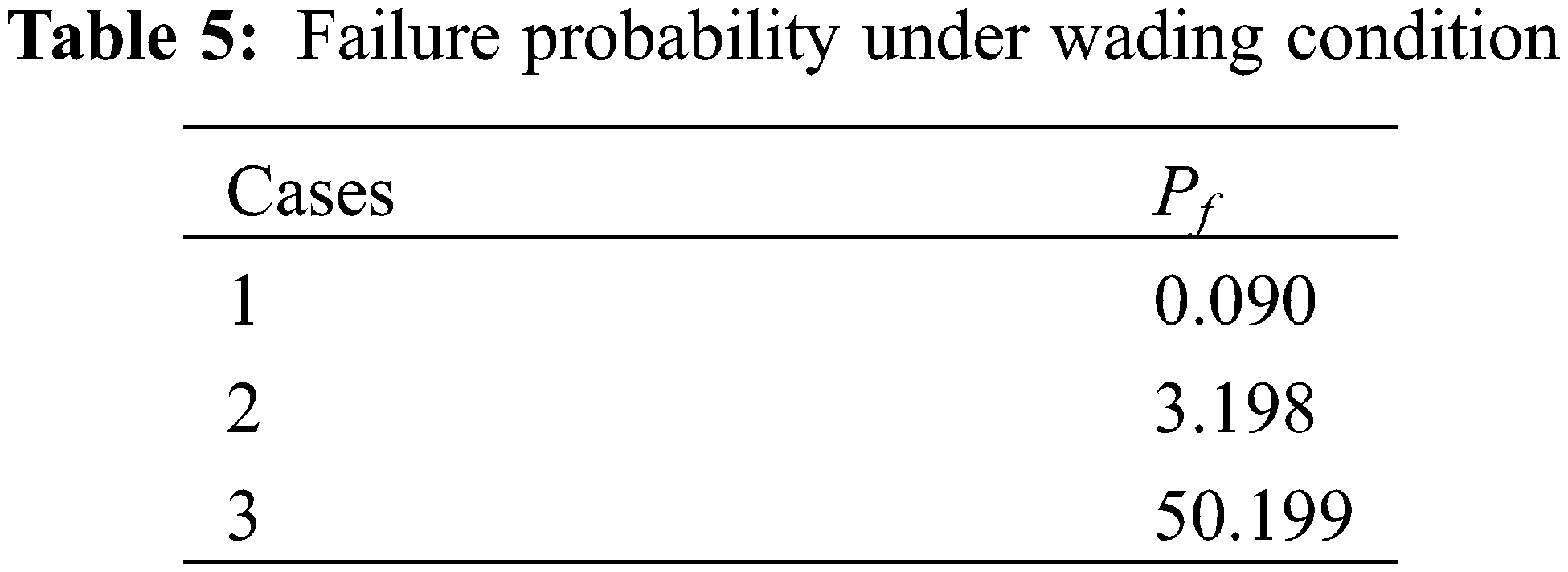
Table 5 presents the outcomes of the three slopes under water-immersed conditions. In three cases, a = 30, v0 = 0.2 m/day, and t = 360 days. It can be observed that for Case 1, the failure probability of the slope under water-immersed condition amounts to 0.09%, which is 25% higher than that under the natural condition. For Case 2, the failure probability of the slope under water-immersed condition is 3.198%, which is 27% higher than that under the natural condition. For Case 3, the failure probability of the slope under water-immersed condition is 50.199%, which is 31% higher than that under the natural condition.
3.2.1 Accuracy and Calculation Time
An exact solution for slope failure probability can be acquired through the MCS method. After 30,000 times of sampling, the failure probabilities of the slopes in Cases 1–3 were 0.074%, 2.582%, and 37.810%, respectively. The errors of the proposed method in comparison with the MCS method are 2.341841%, 2.478699%, and 1.34885% (Table 6). As can be observed, the proposed method possesses high accuracy and can satisfy the requirements of engineering applications.
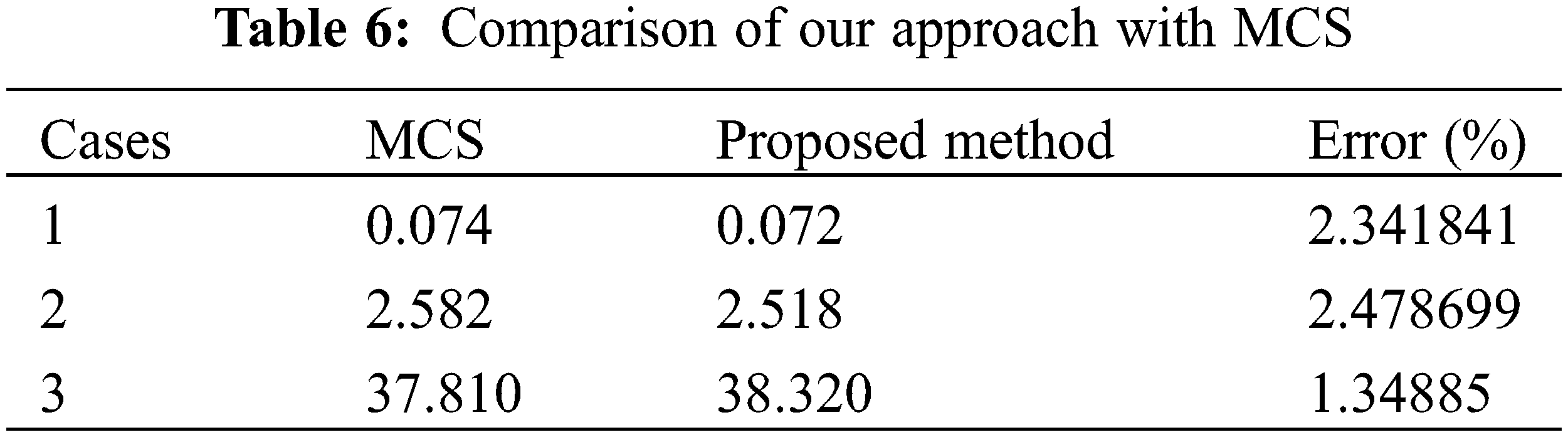
Fig. 9 compares the computation time required for the proposed LSSVM-GWO method and the MCS method across the three case studies (1D, 2D, and 3D slopes). The x-axis represents the different cases, while the y-axis indicates the computation time in seconds. In Cases 1–3, the calculation times of our proposed method are 31.45, 29.17, and 30.33 s, while the times for the MCS method are 0.02, 5260.75, and 83114.99 s (Fig. 9). Except for the 1D slope, our method takes much less time than the MCS algorithm. Since the Fs expression of the 1D slope can be expressed using a simple explicit function, it only takes a short time to calculate Pf directly according to the MCS approach. However, calculation according to the MCS method for 2D and 3D slopes requires much more time. The calculation complexity of the safety factor for 1D to 3D slopes gradually increases. In the calculation of Pf for 2D and 3D slopes, the MCS approach takes 180 times and 2740 times longer than our approach, respectively. The calculation time of our approach is not affected by the complexity of the safety factor model and averages about 30 s. The proposed method has significant advantages over the MCS method in calculating the failure probability of complex slopes.

Figure 9: Comparing the calculation time of this method with the strict MCS method
3.2.2 Comparison of Proposed and Probabilistic Methods
Here, we call the method that does not consider the function of the limit-state a Probabilistic method. Our approach considers the ambiguity of limit-state. Table 3 compares differences between the calculation results of the two. Fig. 10 presents the failure probability results obtained using the proposed LSSVM-GWO method and the classical probabilistic method. The x-axis represents the different cases (1D, 2D, and 3D slopes), while the y-axis indicates the failure probability percentage. According to Probabilistic method, samples were sampled 30,000 times, and the failure probabilities were 0%, 0.040% and 19.550% (Fig. 10). Probabilistic approach is quite different from the proposed approach. In comparison, the probabilistic method underestimates the failure probability of the slope.

Figure 10: Calculation results of the present approach and probabilistic method
3.2.3 Comparison of Different Membership Functions
Except for linear membership rule used in Eq. (2), in fuzzy field, the common membership functions are normal type and Cauchy type [30].
Fig. 11 compares Pf calculation results of the above membership functions used in three cases. The parameter settings are the same as in Section 3.1. As shown in Fig. 11 the difference in the failure probability of several membership functions is relatively small. In contrast, Pf determined by normal membership function is less than the linear function, and Pf by Cauchy membership function is greater than the linear membership function. In practice, using linear membership function is a compromise.

Figure 11: Comparison of different membership functions
This study introduces a novel approach for calculating slope failure probability by incorporating the ambiguity of the limit-state function. The developed method leverages a Least Squares Support Vector Machine (LSSVM) optimized by the Grey Wolf Optimizer (GWO) and K-fold cross-validation to replace traditional limit-state function methods, significantly reducing computational time while maintaining high accuracy.
1. The proposed method was tested on three cases: one-dimensional (1D), two-dimensional (2D), and three-dimensional (3D) slopes. The results demonstrate that the accuracy of our algorithm is exceptional, with an error margin within 3% compared to the strict Monte Carlo Simulation (MCS) method. This accuracy is sufficient to meet engineering requirements, indicating that the alternative model method established in this study is highly reliable and accurate for practical applications. For 1D, 2D and 3D conditions, the probability of failure under wading conditions is 25%, 27%, and 31% higher than that under natural conditions, respectively.
2. One of the significant advantages of the proposed method is its efficiency in reducing computational time, especially for complex limit-state functions. In the calculation of 2D and 3D slope failure probabilities, the proposed method is approximately 180 times and 2740 times faster than the MCS method, respectively. This dramatic reduction in computation time highlights the method’s potential for real-time applications and large-scale simulations where traditional methods would be impractical due to time constraints.
3. Compared with our algorithm, the classical probabilistic methods tend to underestimate the slope failure probability. This disparity highlights the significance of considering the ambiguity in the limit-state function, which our method effectively handles. The incorporation of this ambiguity offers a more realistic and precise estimation of slope failure probabilities, rendering the proposed method superior in scenarios where precision is of vital importance.
4. The type of membership function used in the fuzzy limit-state model significantly influences the calculated failure probability. Our findings show that the failure probability obtained using a linear membership function lies between those derived from normal and Cauchy membership functions. This sensitivity to membership function types suggests that careful selection and tuning of these functions are essential for accurate failure probability estimation.
5. While incorporating the ambiguity from the limit-state function, the method also introduces uncertainty due to human factors, such as the distribution type and parameters of the membership function. This aspect adds a layer of complexity to the analysis but also aligns more closely with real-world conditions where human judgment and variability play a role.
Acknowledgement: The authors gratefully acknowledge the support of Sichuan Hongye Construction Software Co., Ltd. The authors also thank Shaohong Li for his guidance on the calculation method.
Funding Statement: Ministry of Education, Center for Scientific Research and Development of Higher Education Institutions “Innovative Application of Virtual Simulation Technology in Vocational Education Teaching” Special Project, Project No. ZJXF2022110.
Author Contributions: The authors confirm contribution to the paper as follows: study conception and design: Jianing Hao; data collection: Dan Yang; analysis and interpretation of results: Guanxiong Ren, Ying Zhao; draft manuscript preparation: Jianing Hao, Rangling Cao. All authors reviewed the results and approved the final version of the manuscript.
Availability of Data and Materials: The data involved in this study has been provided in the paper.
Ethics Approval: Not applicable.
Conflicts of Interest: The authors declare no conflicts of interest to report regarding the present study.
References
1. Robson E, Milledge D, Utili S, Dattola G. A computationally efficient method to determine the probability of rainfall-triggered cut slope failure accounting for upslope hydrological conditions. Rock Mech Rock Eng. 2022;57(4):2421–43. [Google Scholar]
2. Gupta K, Satyam N, Gupta V. Probabilistic physical modelling and prediction of regional seismic landslide hazard in Uttarakhand state (India). Landslides. 2023;20(5):901–12. doi:10.1007/s10346-022-02013-3. [Google Scholar] [CrossRef]
3. Deng J, Pandey M. Optimal maximum entropy quantile function for fractional probability weighted moments and its applications in reliability analysis. Appl Math Model. 2023;114:230–51. doi:10.1016/j.apm.2022.10.004. [Google Scholar] [CrossRef]
4. Zeng P, Li T, Jimenez R, Feng X, Chen Y. Extension of quasi-Newton approximation-based SORM for series system reliability analysis of geotechnical problems. Eng Comput. 2017;34(2):215–24. [Google Scholar]
5. Cho SE. Probabilistic stability analyses of slopes using the ANN-based response surface. Comput Geotech. 2017;36(5):787–97. [Google Scholar]
6. Ling C, Lu Z, Sun B, Wang M. An efficient method combining active learning Kriging and Monte Carlo simulation for profust failure probability. Fuzzy Set Syst. 2020;387:89–107. doi:10.1016/j.fss.2019.02.003. [Google Scholar] [CrossRef]
7. Abad ARB, Ghorbani H, Mohamadian N, Davoodi S, Mehrad M, Aghdam SK, et al. Robust hybrid machine learning algorithms for gas flow rates prediction through wellhead chokes in gas condensate fields. Fuel. 2022;308:121872. doi:10.1016/j.fuel.2021.121872. [Google Scholar] [CrossRef]
8. Nwazelibe VE, Unigwe CO, Egbueri JC. Testing the performances of different fuzzy overlay methods in GIS-based landslide susceptibility mapping of Udi Province, SE Nigeria. CATENA. 2023;220:106654. doi:10.1016/j.catena.2022.106654. [Google Scholar] [CrossRef]
9. Luo Z, Hu B. Robust design of energy piles using a fuzzy set-based point estimate method. Cold Reg Sci Technol. 2019;168:102874. doi:10.1016/j.coldregions.2019.102874. [Google Scholar] [CrossRef]
10. Valdebenito MA, Beer M, Jensen HA, Chen J, Wei P. Fuzzy failure probability estimation applying intervening variables. Struct Saf. 2020;83:101909. doi:10.1016/j.strusafe.2019.101909. [Google Scholar] [CrossRef]
11. Hwang IT, Park HJ, Lee JH. Probabilistic analysis of rainfall-induced shallow landslide susceptibility using a physically based model and the bootstrap method. Landslides. 2023;20(4):829–44. doi:10.1007/s10346-022-02014-2. [Google Scholar] [CrossRef]
12. Shahabi H, Ahmadi R, Alizadeh M, Hashim M, Al-Ansari N, Shirzadi A, et al. Landslide susceptibility mapping in a mountainous area using machine learning algorithms. Remote Sens. 2023;15(12):3112. doi:10.3390/rs15123112. [Google Scholar] [CrossRef]
13. Li H, Nie X. Structural reliability analysis with fuzzy random variables using error principle. Eng Appl Artif Intel. 2018;67:91–9. doi:10.1016/j.engappai.2017.08.015. [Google Scholar] [CrossRef]
14. Ye S, Fang G, Ma X. Reliability analysis of grillage flexible slope supporting structure with anchors considering fuzzy transitional interval and fuzzy randomness of soil parameters. Arab J Sci Eng. 2019;44(10):8849–57. doi:10.1007/s13369-019-03912-9. [Google Scholar] [CrossRef]
15. Wang L, Xiong C, Wang X, Liu G, Shi Q. Sequential optimization and fuzzy reliability analysis for multidisciplinary systems. Struct Multidiscip Optim. 2019;60(3):1079–95. doi:10.1007/s00158-019-02258-y. [Google Scholar] [CrossRef]
16. Sotoudeh-Anvari A. A critical review on theoretical drawbacks and mathematical incorrect assumptions in fuzzy OR methods: review from 2010 to 2020. Appl Soft Comput. 2020;93:106354. doi:10.1016/j.asoc.2020.106354. [Google Scholar] [CrossRef]
17. Wang GY, Liu J, Wang YZ. Analysis of fuzzy reliability for plane sliding of slope. Rock Soil Mech. 2005;26:283–6. [Google Scholar]
18. Gupta U, Gupta D. Least squares structural twin bounded support vector machine on class scatter. Appl Intell. 2023;53(12):15321–51. doi:10.1007/s10489-022-04237-1. [Google Scholar] [CrossRef]
19. Mirjalili S, Mirjalili SM, Lewis A. Grey wolf optimizer. Adv Eng Softw. 2014;69:46–61. doi:10.1016/j.advengsoft.2013.12.007. [Google Scholar] [CrossRef]
20. Wong TT. Parametric methods for comparing the performance of two classification algorithms evaluated by k-fold cross validation on multiple data sets. Pattern Recogn. 2017;65:97–107. doi:10.1016/j.patcog.2016.12.018. [Google Scholar] [CrossRef]
21. Gao G, Hazbeh O, Davoodi S, Tabasi S, Rajabi M, Ghorbani H, et al. Prediction of fracture density in a gas reservoir using robust computational approaches. Front Earth Sci. 2023;10:1023578. doi:10.3389/feart.2022.1023578. [Google Scholar] [CrossRef]
22. Zeng Q, Zheng M, Huang D. Simulation of moving bed erosion based on theweakly compressible smoothed particle hydrodynamics-discrete element coupling method. Fluid Dyn Mater Process. 2023;19(12):2981–3005. doi:10.32604/fdmp.2023.029427. [Google Scholar] [CrossRef]
23. Qian Q, et al. Simulation of oil-water flow in shale oil reservoirs based on smooth particle hydrodynamics. Fluid Dyn Mater Process. 2022;18(4):1089–97. doi:10.32604/fdmp.2022.019837. [Google Scholar] [CrossRef]
24. Du X, Liu M, Sun Y. Optimization of the internal circulating fluidized bed using computational fluid dynamics technology. Fluid Dyn Mater Process. 2022;18(2):303–12. doi:10.32604/fdmp.2022.016242. [Google Scholar] [CrossRef]
25. Huang H, Li Z, Luo J, Chang Z. On the stability of carbon shale slope under rainfall infiltration. Fluid Dyn Mater Process. 2021;17(6):1165–78. doi:10.32604/fdmp.2021.017256. [Google Scholar] [CrossRef]
26. Altrock CV. Fuzzy logic and neurofuzzy—applications in business and finance prentice hall, New Jersey mathworks (2018a) MATLAB version 9.4.0. Natick, Massachusetts: The Mathworks, Inc.; 1995. [Google Scholar]
27. Nayak J, Swapnarekha H, Naik B, Dhiman G, Vimal S. 25 years of particle swarm optimization: flourishing voyage of two decades. Arch Comput Method E. 2023;30(3):1663–1725. doi:10.1007/s11831-022-09849-x. [Google Scholar] [CrossRef]
28. Singh SK, Chakravarty D. Assessment of slope stability using classification and regression algorithms subjected to internal and external factors. Arch Min Sci. 2023;68(1):87–102. [Google Scholar]
29. Firincioglu BS, Ercanoglu M. Insights and perspectives into the limit equilibrium method from 2D and 3D analyses. Eng Geol. 2021;281:105968. doi:10.1016/j.enggeo.2020.105968. [Google Scholar] [CrossRef]
30. Ribeiro RA. Fuzzy multiple attribute decision making: a review and new preference elicitation techniques. Fuzzy Set Syst. 1996;78(2):155–81. doi:10.1016/0165-0114(95)00166-2. [Google Scholar] [CrossRef]
Cite This Article
 Copyright © 2025 The Author(s). Published by Tech Science Press.
This work is licensed under a Creative Commons Attribution 4.0 International License , which permits unrestricted use, distribution, and reproduction in any medium, provided the original work is properly cited.
 Downloads
 Citation Tools