
 Submit a Paper
 Propose a Special lssue
 Open Access
ARTICLE

Numerical Analysis of Urban-Rail Vehicle/Tunnel Aerodynamic Interaction
1 Beijing Infrastructure Investment Co., Ltd., Beijing, 100101, China
2 Beijing Rail Transit Technology Equipment Group Co., Ltd., Beijing, 100070, China
3 Department of Mechanical Engineering, Tsinghua University, Beijing, 100084, China
4 State Key Laboratory of Rail Transit Vehicle System, Southwest Jiaotong University, Chengdu, 610031, China
* Corresponding Author: Tian Li. Email:
Fluid Dynamics & Materials Processing 2025, 21(1), 161-178. https://doi.org/10.32604/fdmp.2024.055389
Received 25 June 2024; Accepted 27 August 2024; Issue published 24 January 2025
 View Full Text
 Download PDF
Abstract
The pressure wave generated by an urban-rail vehicle when passing through a tunnel affects the comfort of passengers and may even cause damage to the train and related tunnel structures. Therefore, controlling the train speed in the tunnel is extremely important. In this study, this problem is investigated numerically in the framework of the standard k-ε two-equation turbulence model. In particular, an eight-car urban rail train passing through a tunnel at different speeds (140, 160, 180 and 200 km/h) is considered. The results show that the maximum aerodynamic drag of the head and tail cars is most affected by the running speed. The pressure at selected measuring points on the windward side of the head car is very high, and the negative pressure at the side window of the driver’s cab of the tail car is also very large. From the head car to the tail car, the pressure at the same height gradually decreases. The positive pressure peak at the head car and the negative pressure peak at the tail car are greatly affected by the speed.Keywords
Nomenclature
| A | Maximum cross-sectional area of the train |
| Cd | Coefficient of aerodynamic drag |
| Cp | Coefficient of pressure |
| Fd-max | Maximum aerodynamic drag |
| Lt | The length of the tunnel |
| Lv | The length of the vehicle |
| M | Mach number |
| Tx | Tunnel factor |
| V | Train speed |
| Ρ | Air density |
The increasing speeds of urban rail vehicles can lead to a reduction in aerodynamic performance, so many scholars have studied the aerodynamic performance of rail vehicles. Academics at the University of Birmingham and Politecnico di Milano have performed numerical simulations and experimental studies of the aerodynamic performance of trains in crosswinds and tunnels [1–4]. The Eindhoven University of Technology investigated the wind conditions during the passage of trains through underground tunnels and platforms by using Computational Fluid Dynamics (CFD) [5]. As the running speed increases, the aerodynamic performance of the vehicle as it passes through the tunnel increases significantly [6]. When a train enters a tunnel at high speed, it generates a series of continuously propagating pressure waves [7]. The pressure waves cause a sharp change in pressure on the tunnel wall and the train body, which in turn produces a series of aerodynamic effects. Factors such as train speed [8], head shape [9,10], and tunnel structural parameters [11,12] have a significant impact on the aerodynamic performance of a train passing through a tunnel.
At present, the academic and engineering communities have conducted extensive research on the impact of train speed on aerodynamic performance when a train passes through a tunnel. The main research methods currently include theoretical investigation, full-scale tests, scaled model experiments, and numerical simulations [13–16]. Negri et al. [17] investigated the effect of trains air flow speeds through a full-scale experiment, analyzing the effect of different train parameters and infrastructure parameters on the slipstream generated by trains passing through tunnels. Zhang et al. [18] used a 1:20 scale model to analyze the effect of a train’s speed on the peak pressure on the train surface. Compared with experiments, the use of numerical simulation to study the aerodynamic performance of trains can significantly reduce time and cost. Currently, Direct Numerical Simulation (DNS), Reynolds-Averaged Navier-Stokes (RANS), Large-Eddy Simulation (LES), and RANS-LES are mainly used for the numerical simulation of ground vehicles. Since DNS is not only costly but also has a very long cycle time, it is ill-suited to solving the complex turbulence problems encountered in engineering. Therefore, RANS and LES, which can solve these engineering problems more easily, have been used more often. The RANS-LES method combines the advantages of the RANS and LES methods, and the simulation of the separated flow effect is much better than that of the RANS method alone [19–22]. Rabani et al. [23] investigated the effect of train speed on pressure waves, drag, and lateral forces, by using numerical simulations. Zhou et al. [24] studied the aerodynamic performance of a train passing through a tunnel in three different speed modes (350 km/h uniform speed, 350–300 km/h uniform deceleration, and 350–250 km/h uniform deceleration). They found that when a train passes through a tunnel in a uniform deceleration mode, the peak pressures on the tunnel, and on the train surface were reduced by 15.8% and 12.8%, respectively. Train speed also has a significant impact on the surface pressure characteristics of tunnels [18,25]. Liu et al. [26] conducted on-site measurements of the surface pressure on a 2812 m tunnel, and found that as the train speed increased, the position of the maximum value of the peak-to-peak pressure gradually moved toward the tunnel entrance. When two trains meet in a tunnel, the influence of train speed on aerodynamic performance is greater than that of track spacing or vehicle size [27].
A large pressure drop inside the vehicle as it passes through the tunnel causes discomfort to the passengers inside [28,29]. The operating speed of urban rail vehicles will significantly affect the auditory comfort of passengers. Xiong et al. [30] conducted on-site tests on the effect of subway train speed on the pressure changes inside and outside the train, and found that the pressure change inside the train is proportional to the train speed, with a power exponent of 1.5~1.6. Sun et al. [31] studied subway tunnels in terms of the pressure comfort of passengers, and determined the critical diameter of tunnels at different operating speeds. Yang et al. [32] used numerical simulation methods to study the differences in aerodynamic characteristics of subway trains in tunnels, both when they are at a constant speed, and when they are accelerating or decelerating. This provides a theoretical basis for wind energy resource recovery and fan layout, in tunnels.
With the continuous development of urban rail systems, especially high-speed urban rail, higher requirements have been put in place for aerodynamic performance. Therefore, it is necessary to conduct specific in-depth research on different vehicles, routes, and operating environments, to select the optimal operating speed, while ensuring passenger comfort and operational economy. This article aims to analyze the aerodynamic performance of a certain type of eight-marshaling urban rail vehicle, passing through tunnels at different speeds. This is to explore the relationship between its aerodynamic force and surface pressure, and speed, providing the theoretical basis for the design and operation of urban rail vehicles.
2.1 Geometric Model and Boundary Conditions
A specific type of urban rail train is taken as the research object, and its operation in the tunnel is numerically calculated. The geometric models used for calculation are the train model and the tunnel model. A whole eight-marshaling train model is used for numerical simulation. The model consists of a head car and a tail car, 6 middle cars, 7 windshields, and 16 bogies. The head cover and appearance of the leading and trailing cars are the same. The model of the train is shown in Fig. 1. The length of the head and tail cars is about 24.50 m, the length of the middle cars is about 22.00 m, the windshield length is 0.80 m, and the total length of the train is about 186.60 m. The height of the train is about 3.81 m, the width is about 3.27 m, and the maximum cross-sectional area of the train body is about 11.78 m2.
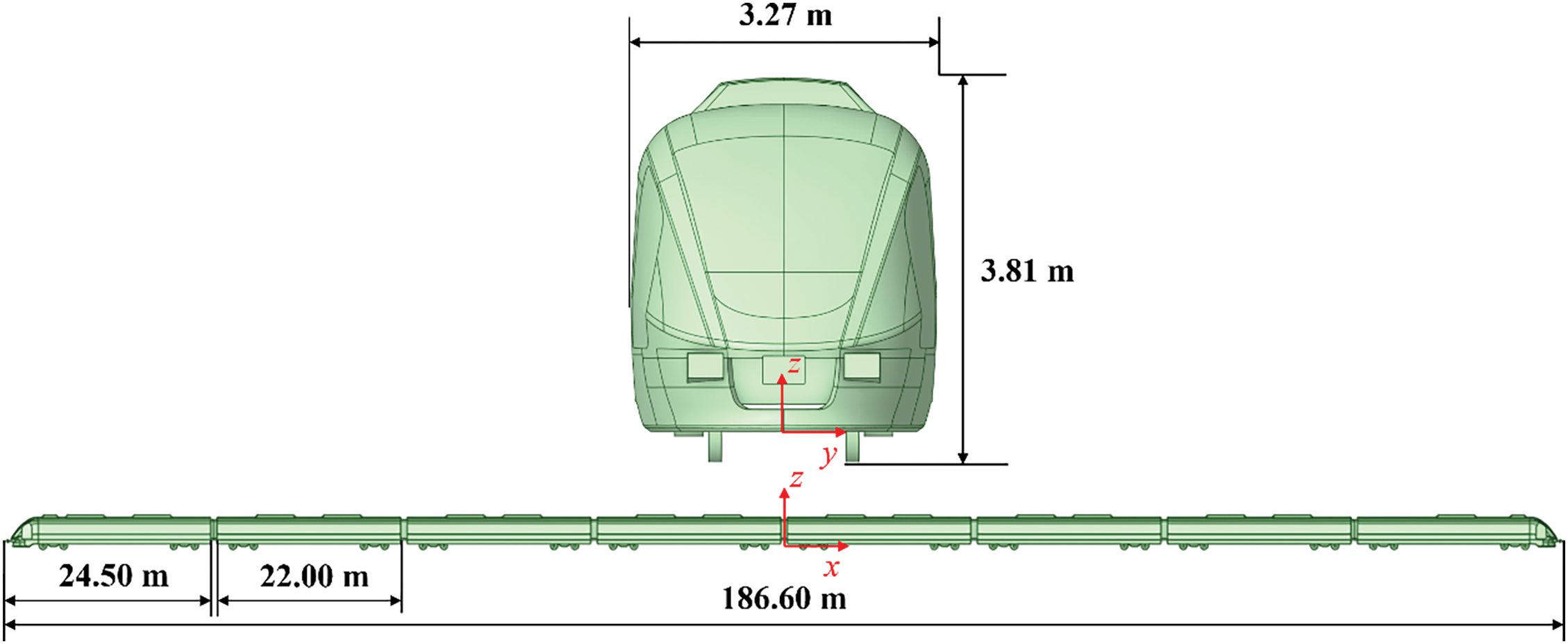
Figure 1: Train model
The aerodynamic performance of a train passing through a tunnel is related to the length of the tunnel. There is a most unfavorable tunnel length, which causes undesirable aerodynamic performance when the train passes through. The formula for the most unfavorable tunnel length is as follows [33]:
where, Lt and Lv are the lengths of the tunnel and the train, respectively, and M is the operating Mach number.
According to Eq. (1), the most unfavorable tunnel length is about 1026 m when the train passes through at 140 km/h. The most unfavorable tunnel lengths calculated at 160, 180, and 200 km/h are smaller than those calculated at 140 km/h, so the tunnel model with a length of 1026 m is used in the numerical simulation. As shown in Fig. 2a, the atmospheric environment before and after the tunnel is simulated using a rectangular cross-section of an external flow field region with a length of 350 m, a width of 60 m, and a height of 40 m. At the starting point, the nose of the train is 80 m away from the entrance of the tunnel, which provides a certain amount of space for the development of turbulence before the train reaches the entrance of the tunnel. Fig. 2b shows the boundary conditions when the train passes through the tunnel, and the boundary conditions of the two outer computational domains are set to be exactly the same. The two side and top faces are set as symmetric surfaces, and the rest of the faces and the tunnel walls are set as no-slip walls. A standard wall roughness model was used, with a roughness height of 0, and a roughness constant of 0.5.
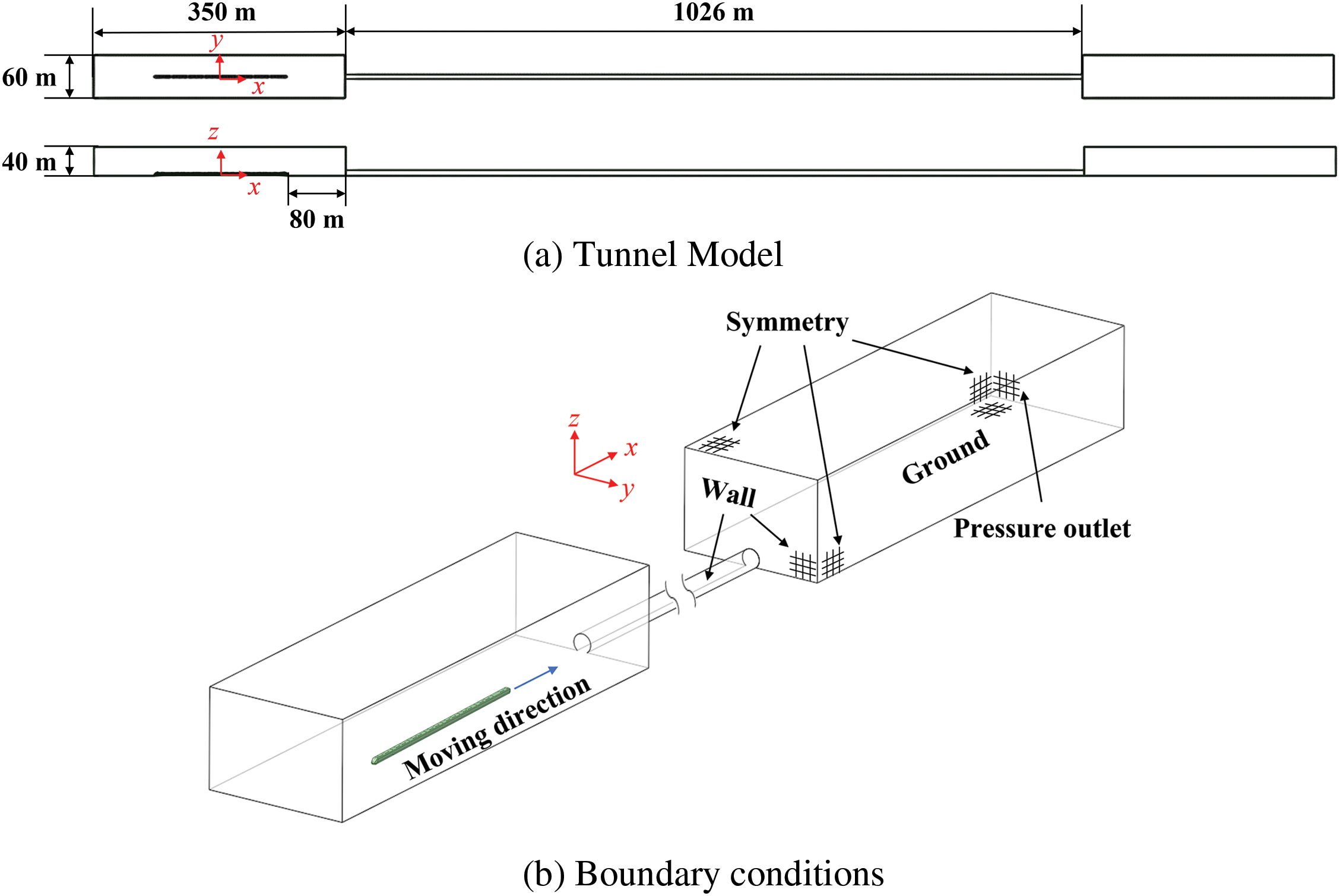
Figure 2: Tunnel Model and boundary conditions
The slip grid is used to simulate the relative movement of the train and the tunnel area. The whole flow field area grid is divided into a moving region and a static region, the grid around the train slips at the train’s running speed, the static region includes the tunnel area and the external flow field area of the tunnel, and the grid information of the static region and the moving region is transferred through the interface. Fig. 3 shows the schematic diagram of the computational area partition and boundary condition settings, for when the high-speed train passes through the tunnel.
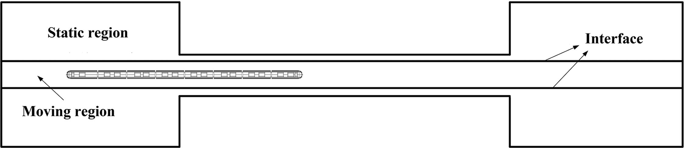
Figure 3: Schematic diagram of tunnel flow zones
In this paper, the commercial software Fluent is used for numerical calculations. The flow field near the wall is simulated using the standard wall function approximation. Numerical calculation modeling using the standard k-ε two-equation turbulence model, in conjunction with the standard wall function, can give more accurate results [34,35]. For numerical calculations, the residual tolerance is 10−3 for the continuity equation, 10−6 for the energy equation, 10−3 for the velocity equation, and 10−3 for both k and ε. The Semi-Implicit Method for Pressure Linked Equations (SIMPLE) algorithm is used to solve the flow field and pressure.
The ICEM CFD software is used to mesh the fixed and moving regions of the flow field, with a body mesh size of 3000 mm for the fixed region, 750 mm for the moving region, and a maximum mesh of 80 mm for the train surface, all of which are meshed by tetrahedral meshes. A total of eight boundary layer meshes are used near the train surface, with the first layer having a height of 1 mm and a growth rate of 1.2, to satisfy y+ in the range of 30 to 300. The number of meshes in the static region is about 7 million, the number of meshes in the moving region is about 24.39 million, and the overall number of meshes is about 31.39 million. In addition, to validate the effect of the number of meshes on the simulation results, two other finite element models with different numbers of meshes were divided, with mesh numbers of 22.34 million and 48.34 million, respectively. The three sets of meshes are named Mesh 1, Mesh 2, and Mesh 3, in descending order of mesh quantity. The computational meshes are shown in Fig. 4.
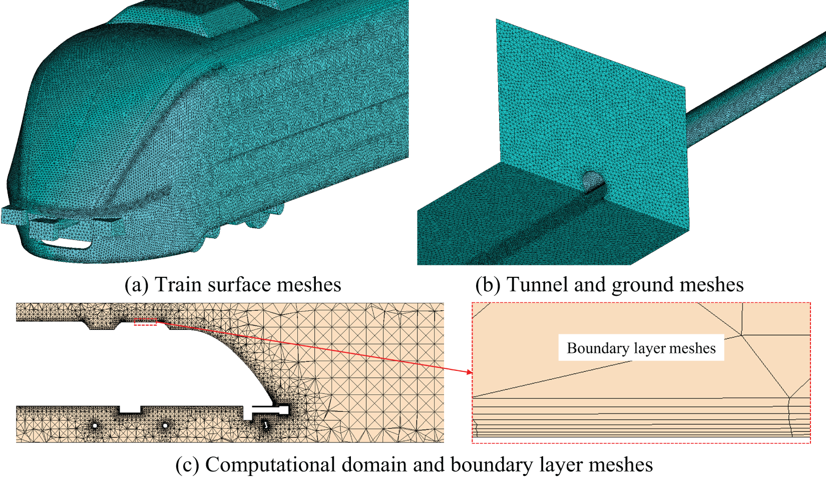
Figure 4: Computational meshes
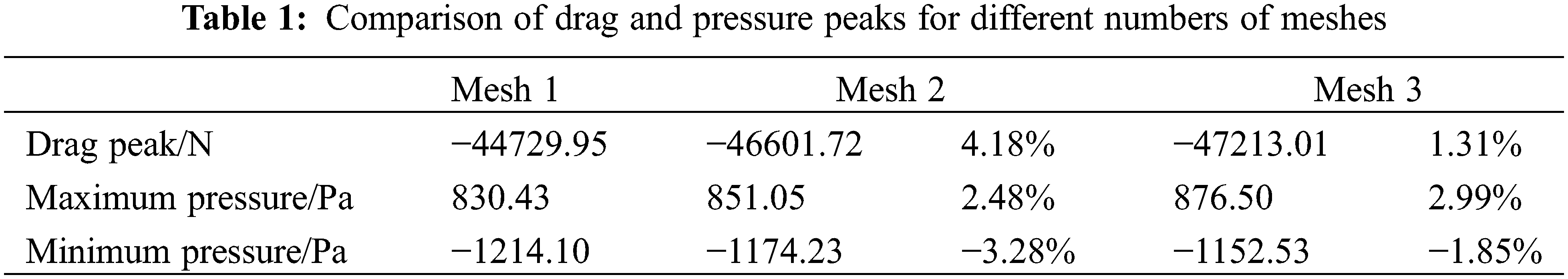
Fig. 5 shows the train drag and pressure curves obtained by simulation, with different numbers of meshes. It can be seen that as the number of meshes increases, the curve differences between different meshes gradually decrease, and the pressure curves between Mesh 2 and Mesh 3 are essentially the same. Table 1 gives the comparison results of the drag peak and pressure peak for different numbers of meshes. The peak difference between Mesh 1 and Mesh 2 is given in the Mesh 2 column in the table, and the peak difference between Mesh 2 and Mesh 3 is given in the Mesh 3 column. As the number of meshes gradually increases, the peak difference gradually decreases. As this occurs, the difference between the drag peaks decreases from 4.18% to 1.31%, the difference between the minimum pressure values decreases from 3.28% to 1.85%, and the difference in the maximum pressure value increases slightly, but does not exceed 3%. It can be seen that the results calculated by Mesh 2 and Mesh 3 are relatively accurate. Considering the need for both calculation accuracy and calculation speed, the mesh size of Mesh 2 is used for mesh division in subsequent calculations.
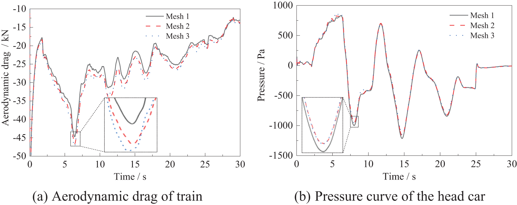
Figure 5: Comparison of results with different numbers of meshes
Since the train used in this paper has not been tested on a railway line, and there is no experimental data to validate the numerical simulation, numerical simulation is carried out using a train model from the literature [36], and compared with the experimental values, to verify the reliability of the numerical simulation. A comparison of the pressure results of the pressure measurement point at the middle point of the second car of the train, with the results of the scaled model test from the literature, is shown in Table 2 and Fig. 6.
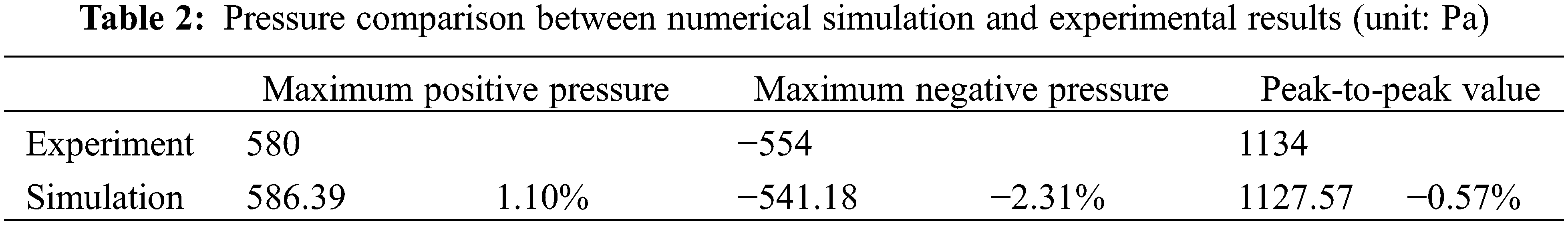
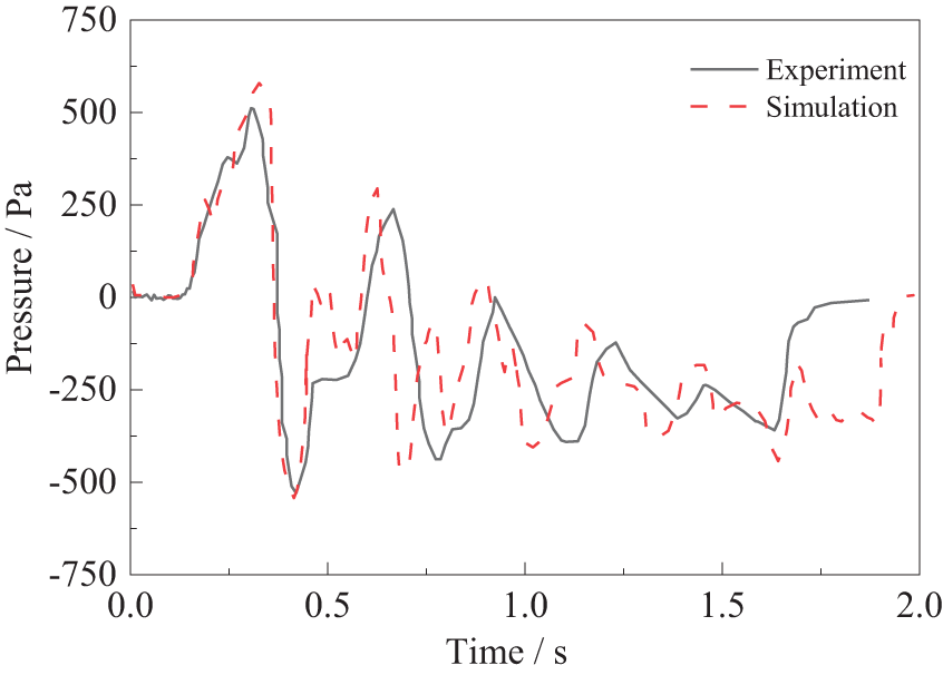
Figure 6: Comparison of pressure curves at the carriage measurement point
It can be seen that the numerical simulation and test of the pressure curve change rule are essentially the same and that only the pressure size is different. The maximum relative error between the numerical simulation and the test results is only 2.31%, and the difference in peak-to-peak values is less than 1%, which is within the acceptable error tolerance of numerical calculation. The deviation in the peak time may be due to a slight variation in test speed and higher temperature, present in the experiment. The above findings demonstrate the accuracy of the numerical method in this paper, which can be used for subsequent research.
This paper mainly studies the effect of running speed on the aerodynamic performance of the train passing through the tunnel, for which, numerical simulations of the train running at speeds of 140, 160, 180, and 200 km/h were carried out. The influence of running speed on aerodynamic performance is analyzed in terms of the change rules of train aerodynamic force and of surface pressure.
The aerodynamic force on the train passing through the tunnel is calculated based on an area-integrated approach to determining the pressure on the outer surface of the train. The train runs in the +x direction, so the numerically calculated resistance is along the −x direction, and is therefore negative. The aerodynamic drag of the train is affected by the compression wave and expansion wave, under which the aerodynamic drag increases and decreases. Fig. 7 shows the corresponding relationship between the change of drag of the head car and the propagation of the Mach wave, when the train passes through the tunnel at 140 km/h. The red line in the graph represents a compression wave, leading to an increase in resistance, and the blue line represents an expansion wave, leading to a decrease in resistance. The number symbols in the graph represent the moment in time when the head car meets the pressure wave. It can be seen that the head car generates a compression wave at the moment ① (as it enters the tunnel), resulting in an increase in the resistance of the head car. This compression wave returns, to generate an expansion wave when it reaches the tunnel exit. Since the tunnel length is exactly that of the most unfavorable tunnel length for the train at that speed, this expansion wave is superimposed with the expansion wave generated when the tail car enters the tunnel at the moment ②, which leads to a decrease in the drag of the head car. Subsequently, due to the back-and-forth propagation of the compression wave and the expansion wave, the drag of the head car is caused to rise and fall.
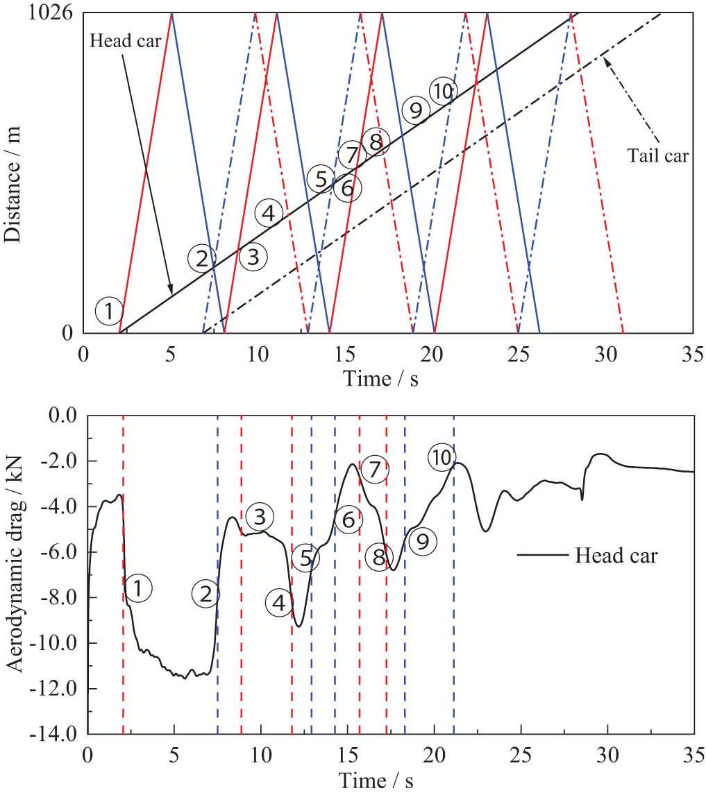
Figure 7: Correspondence between drag variation and Mach wave propagation for head car
Table 3 gives the variation of aerodynamic drag as the train passes through the tunnel at a speed of 160 km/h. When the train is running outside the tunnel, the drag of the head car is −4179.34 N, the drag of the tail car is −3259.19 N, and the drag of the whole train is −16136.16 N. When the train is running in the tunnel, the peak aerodynamic drag of the head car is −15146.23 N, and the average drag is −7260.76 N. The peak aerodynamic drag of the tail car is −10661.00 N, and the average drag is −6002.74 N. The peak aerodynamic drag of the whole car is −46601.72 N, and the average drag is −25232.94 N.
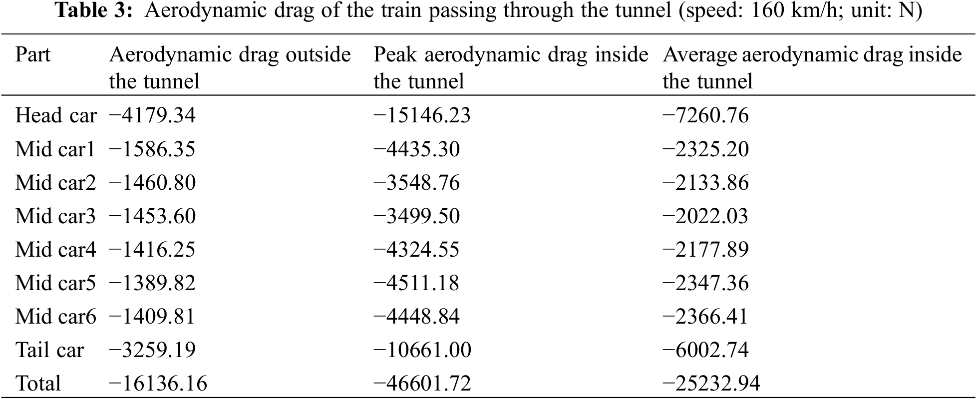
Table 4 shows the factor of aerodynamic drag increase when the train runs in the tunnel. After the train enters the tunnel, the peak aerodynamic drag of the whole car increases by about 2.89 times, with the head car having the largest peak drag value, being 3.62, followed by the tail car, at 3.27. The average drag of the whole car increases by about 1.56 times, with the tail car having the largest average drag at 1.84, followed by the head car at 1.74. It can be seen from the table that the drag of the head car accounts for the largest proportion of the whole car, followed by the tail car, and considering that the head and tail car have a larger increase in drag after entering the tunnel, the head and tail car should be focused upon.
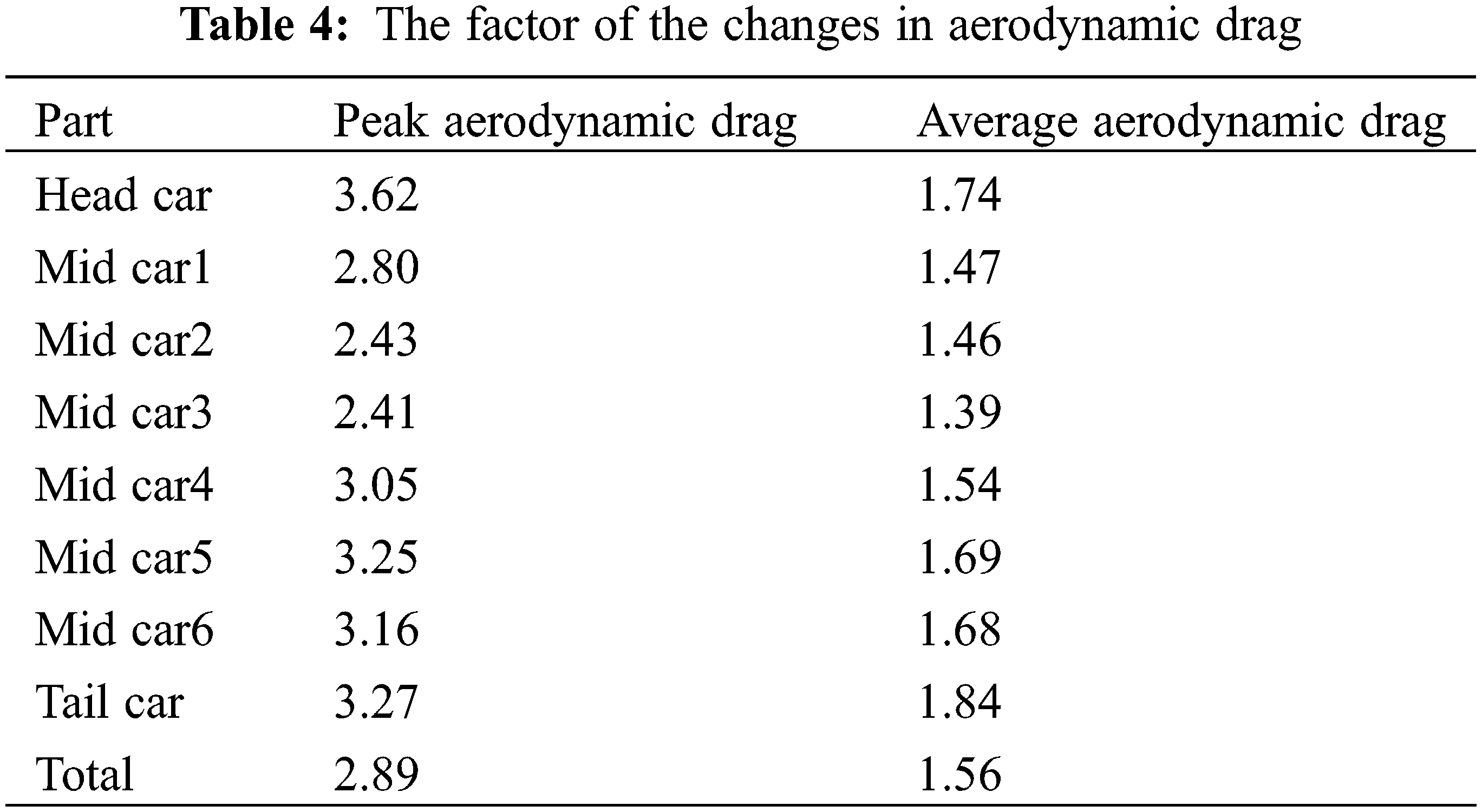
Fig. 8 shows the variation of aerodynamic drag of trains at different speeds. As can be seen, the change rule of aerodynamic force for the train passing through the tunnel is fairly consistent for different speeds. Due to the aerodynamic drag changing at different times, when passing through the tunnel at different operating speeds, the peak drag appears at different moments. Overall, the aerodynamic force generated is greater when the train passes through the tunnel at a higher speed.
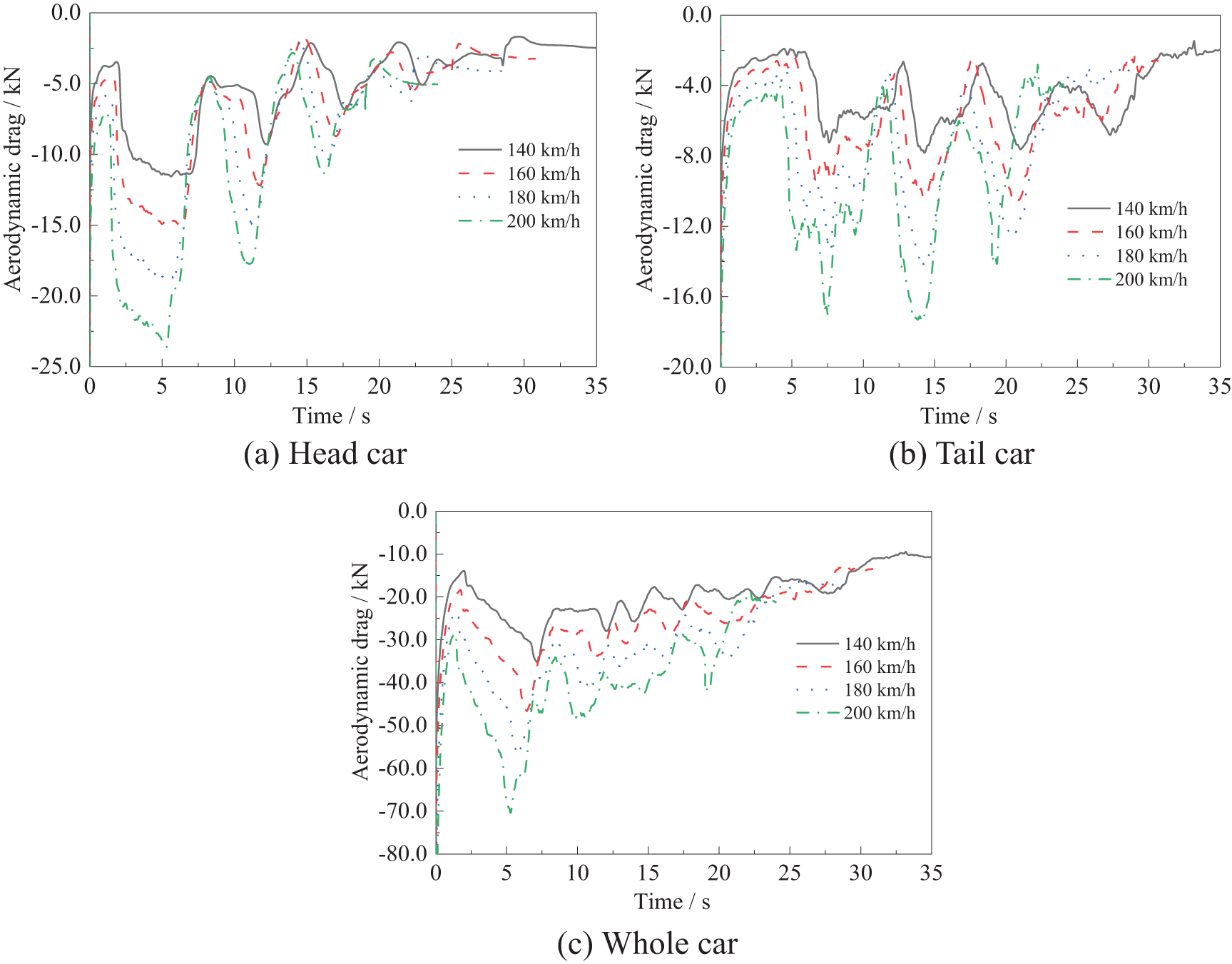
Figure 8: Variation of aerodynamic drag of trains at different speeds
Table 5 shows the variation of peak aerodynamic drag of the train at different speeds. Compared to the whole car drag at an operating speed of 140 km/h, the whole car drag increases by 32.16%, 61.60%, and 99.66%, at operating speeds of 160, 180, and 200 km/h, respectively. It can be concluded from the analysis that the peak drag is proportional to the square of the speed magnitude when the train is running at different speeds. Therefore, the maximum drag Fd-max (unit: N) of the head and tail car, a typical mid car, and the whole car, is fitted to the relationship with the speed of the car V. The fitted function coefficients shown in Table 6 are obtained by fitting using Eq. (2). These R2 of the fitted equations for the peak drag of the head car, mid car and the whole car are above 0.99, which indicates the reasonableness of the fitted equations.
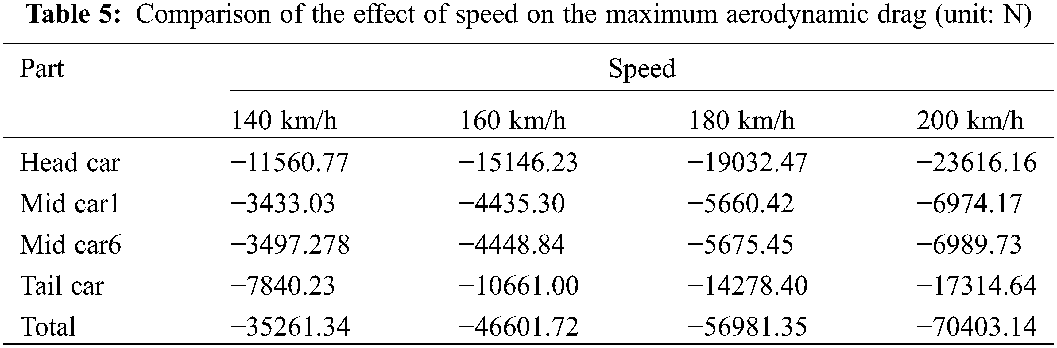
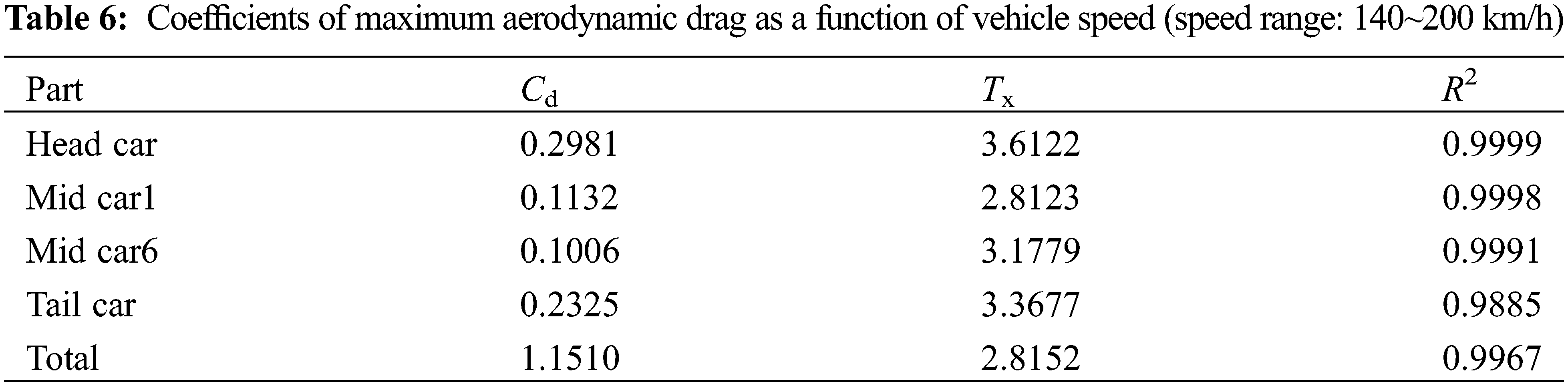
where, Tx is the tunnel factor, ρ is the air density (1.205 kg/m3), A is the maximum cross-sectional area of the train (11.78 m2), V is the running speed of the train, and Cd is the coefficient of aerodynamic drag of the train when it is running in the open air.
Fig. 9 gives the variation of aerodynamic lift of the head and tail car as the train passes through the tunnel. It can be seen that at the moment when the train enters, and the moment when the train leaves the tunnel, the lift of the head car changes significantly, and the original downward aerodynamic lift decreases and then increases. When the train is running in the tunnel, changes in the lift of the head car are small, and the lift is negative throughout tunnel passage. The aerodynamic lift of the tail car increases sharply and then decreases, after entering the tunnel, and there are also large fluctuations in the aerodynamic lift during operation, but the general trend of the change in the lift of the tail car is a gradual decrease. The aerodynamic lift change rules of the train passing through the tunnel with different running speeds are essentially the same, and only the change of aerodynamic force is different in timing and size. The larger the running speed of the train, the larger the aerodynamic lift and the lift amplitude generated when passing through the tunnel, and the more obvious the aerodynamic performance.
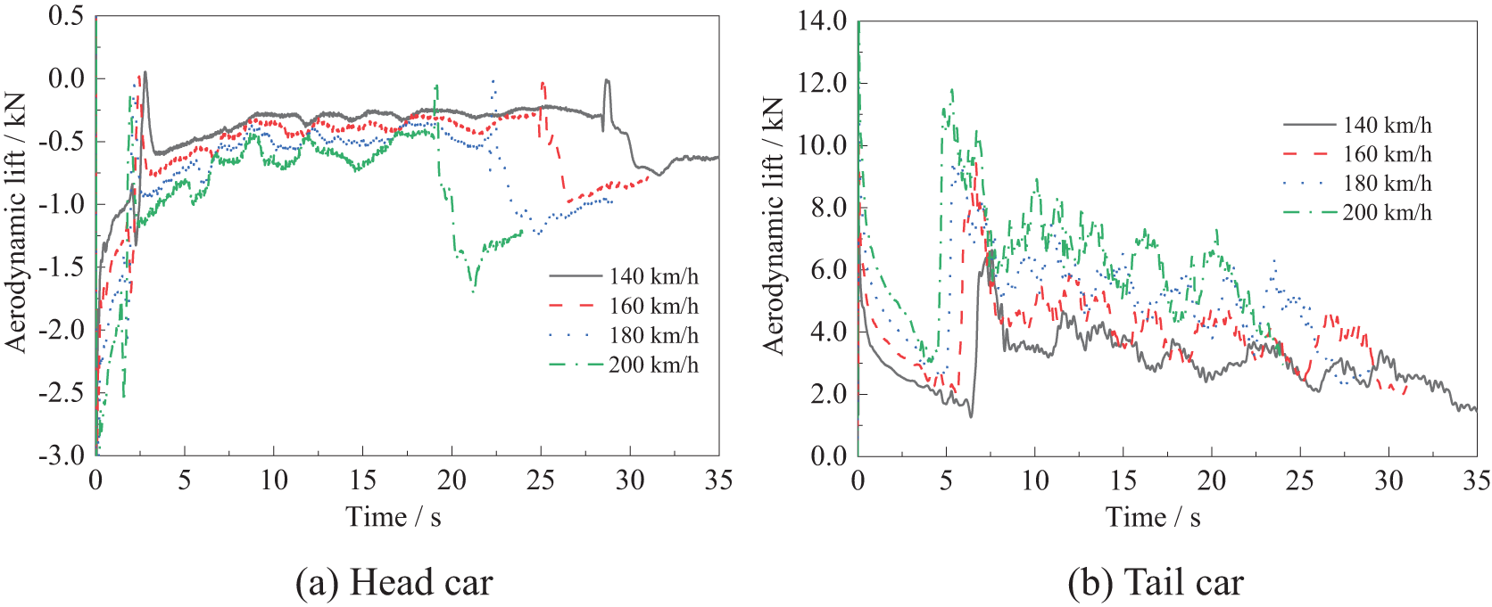
Figure 9: Variation of aerodynamic lift of trains with different speeds
To study the relationship between the pressure changes on the surface of the car body when the train passes through the tunnel, the streamlined hood and body of the head and tail car, and the body of the mid car of the train calculation model are taken respectively as the pressure measurement points in Fig. 10. The streamlined hood sections of both the head and tail car are each equipped with five measurement points. In the head car, these are located at the hood (HP-CG), the nose (HP-NT), the front glass of the driver’s compartment (HP-NW1), and the left and right side windows of the driver’s compartment (HP-NW2, HP-NW3). Seven measurement points are arranged in the body cross-section, numbered HP-B1~7. The tail car measurement points are located in corresponding locations and are numbered with the prefix TP. There are a total of six mid cars, each having a cross-sectional arrangement of seven measurement points, numbered MP#-B1~7.
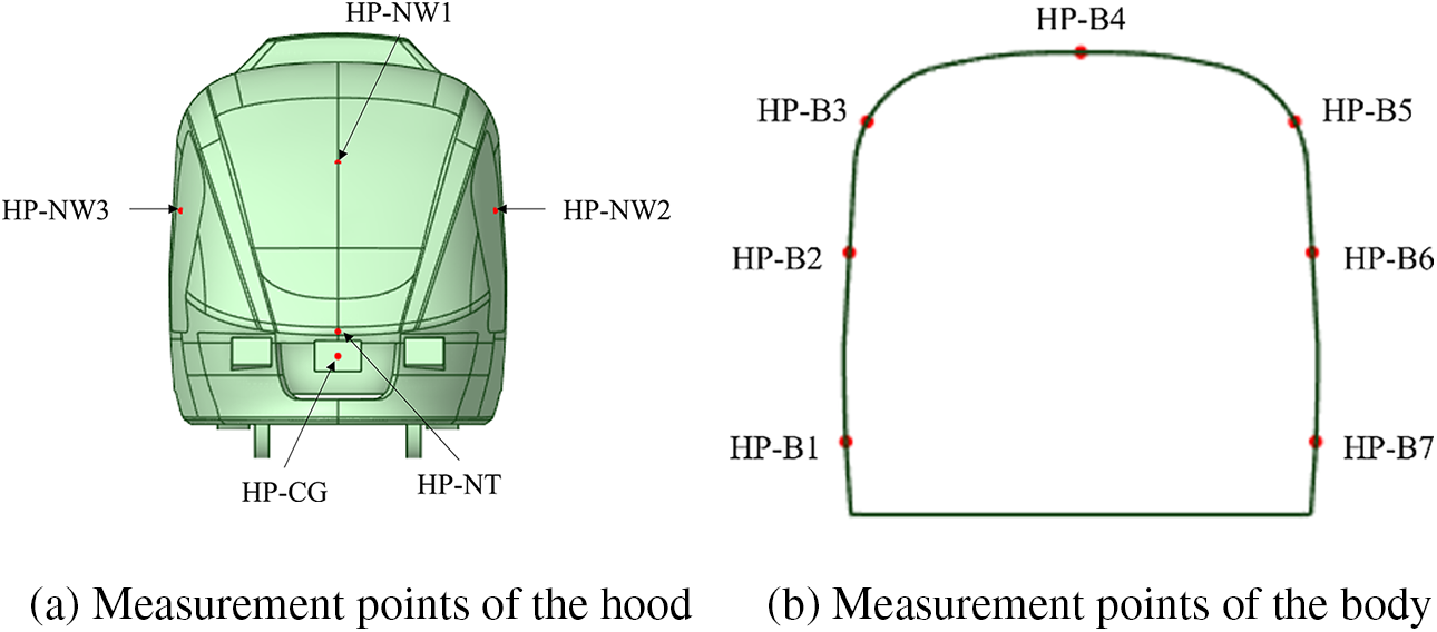
Figure 10: Schematic layout of pressure measurement points
Fig. 11 shows the pressure changes at different locations on the train surface when the train passes through the tunnel at 160 km/h. This is used as an example, to analyze the pressure distribution law at different locations on the train surface. Typical measurement points are selected to analyze the pressure changes at different operating speeds.
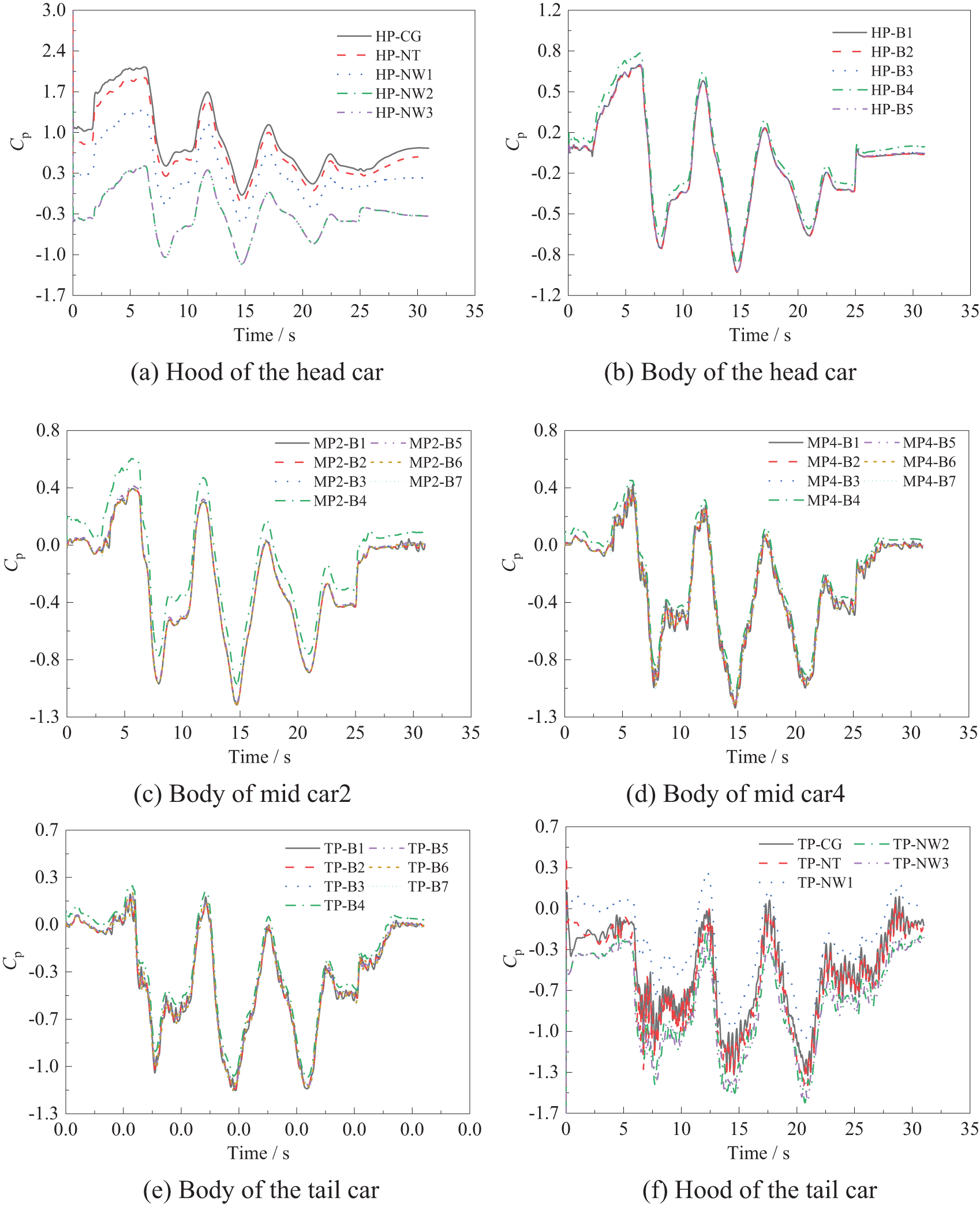
Figure 11: Changes in pressure patterns at surface measurement points
It can be seen from Fig. 11, that, as the windward side of the train, the head car hood has the largest positive pressure amplitude, followed by the nose of the head car, and the driver’s room windshield. The driver’s room left and right side windows pressure change laws, and the size of the changes, are essentially the same. In the body section, due to the air conditioning unit causing the airflow separation and then reattachment to the top of the body, the pressure on the top of the body is greater than the pressure on other parts of the body. The position of the symmetry of the body pressure curve is essentially the same. Due to the attachment of the airflow, the positive pressure on the windshield of the driver’s compartment of the tail car is the largest, the pressure change rule of the windows on both sides is the same, and the negative pressure peak of the side window of the tail car is the largest, due to the fact that the side window of the tail car is located in the transition part of the streamline, where the airflow forms a larger separating vortex. Therefore, in the design and operation of the vehicle, we need to pay attention to the driver’s cab front window of the head car, and the driver’s cab side window of the tail car.
Fig. 12 shows the change rule of pressure at the measurement point on the left side of the train body along the running direction and studies the change rule of body pressure from the head car to the tail car. It can be seen that, along the direction of the head car to the tail car, the value of the pressure at the same height of the body gradually decreases, the positive pressure value of the body of the head car is the largest, while the negative pressure value of the body of the tail car is the largest. The pressure value of the body of the head car increases the fastest during the period from the moment t1, when the compression wave is encountered, to t2, when the expansion wave is encountered, and that the rate of change of the pressure value decreases in the direction from the head car to the tail car.
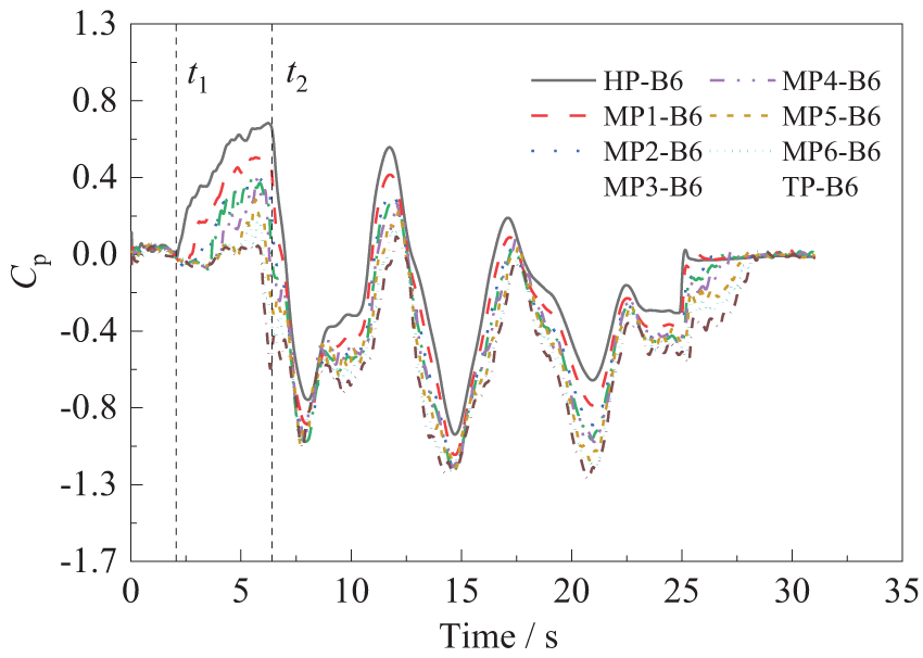
Figure 12: Train single-side pressure along the running direction change law
Some typical measurement points on the surface of the hood and body were selected, to analyze the influence of running speed on the surface pressure when the train passes through the tunnel, and the pressure change process of typical measurement points on the surface of the train under different speed conditions is shown in Fig. 13.
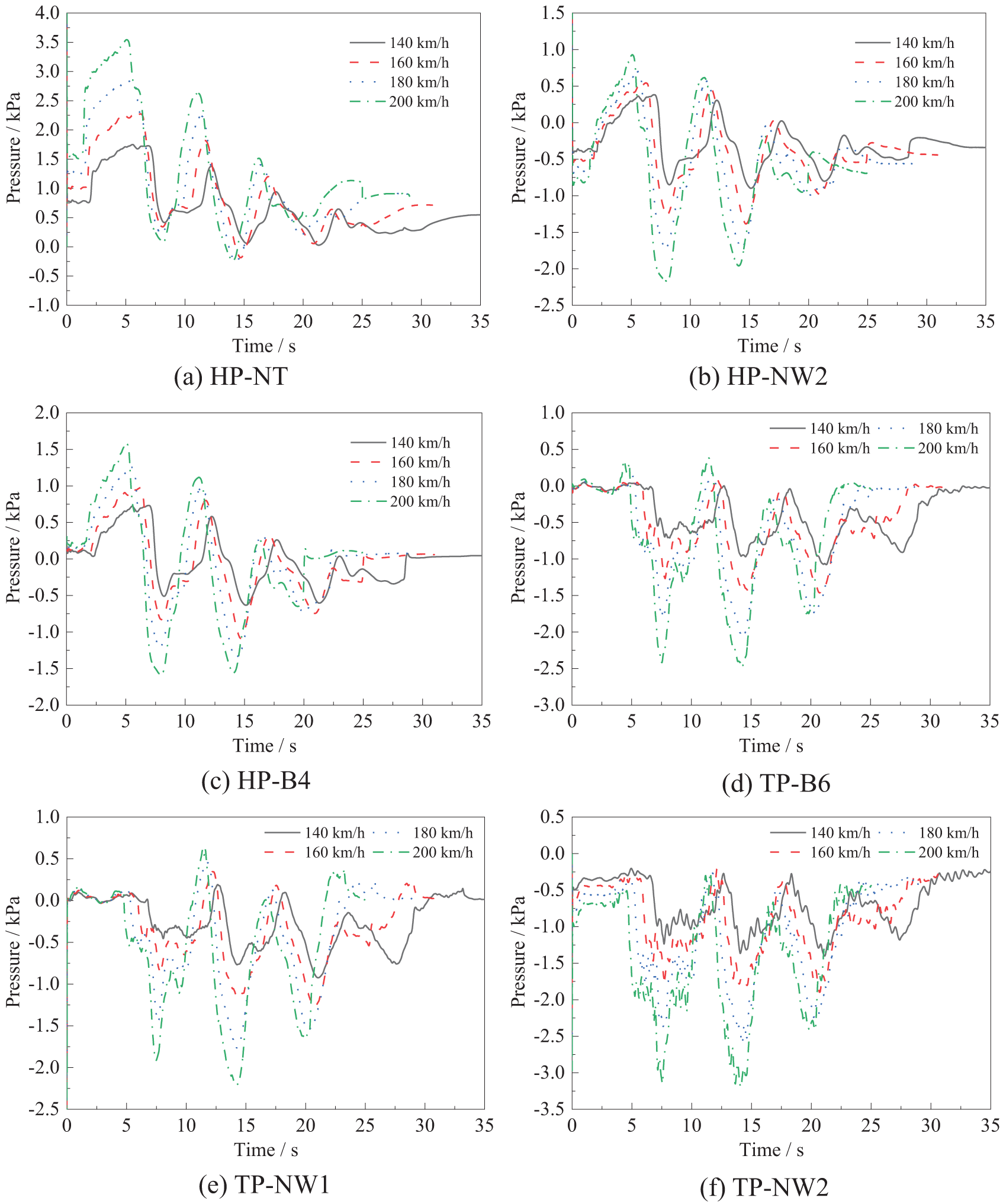
Figure 13: Comparison of the pressure at the measurement points when the train passes through the tunnel at different speeds
As can be seen from Fig. 13, when the train passes through the tunnel at different speeds, the change law of the train surface is essentially the same, such that only the moment of pressure change and pressure amplitude are different. The higher the train speed, the more significant the tunnel aerodynamic effect, and the higher the amplitude of the train surface pressure. The peak positive pressure at the nose tip of the head car varies significantly with speed, while the change in negative pressure is relatively insignificant, and the peak positive and negative pressures at points HP-NW2 and HP-B4 vary more significantly with speed. The peak negative pressure at the measurement point of the tail car varies considerably with speed, and the change in positive pressure is relatively insignificant.
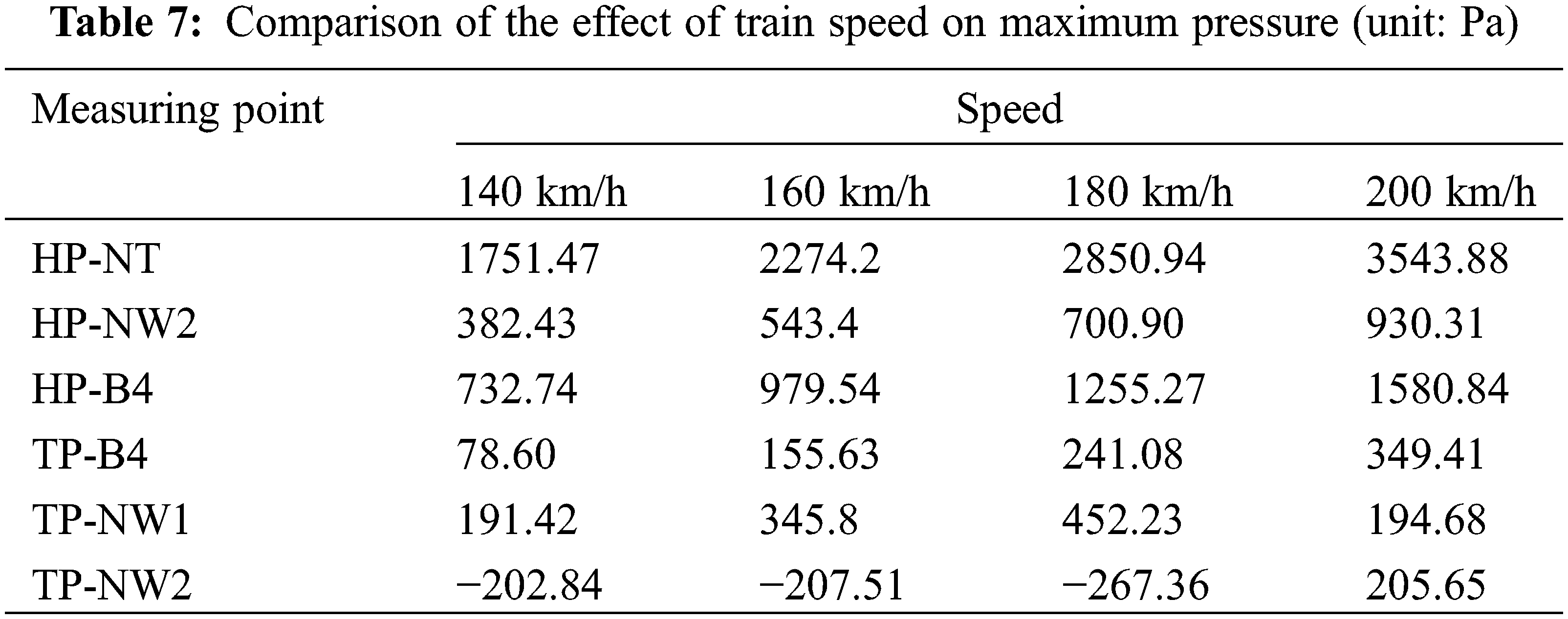
To further illustrate the effect of running speed on the magnitude of train surface pressures, Tables 7 and 8 give the variation of maximum and minimum pressures at typical measurement points on the surface of the head and tail cars of the train, as the train passes through the tunnel at different speeds. As can be seen from Tables 7 and 8, the amplitude of both positive and negative pressures at the measurement points on the car body increases with increasing speed, but the minimum pressure value at the nose tip of the head car and the maximum pressure value of the tail car is less affected by the speed, and the changes are relatively insignificant. Compared to the pressure at the measurement points at a running speed of 140 km/h, the positive pressure amplitudes at the nose tip measurement point with the largest positive pressure values are increased by 29.85%, 62.77%, and 102.34%, respectively, and the negative pressure amplitudes at the tail car view window measurement point with the largest negative pressure values are increased by 35.41%, 86.28%, and 128.15%, respectively.
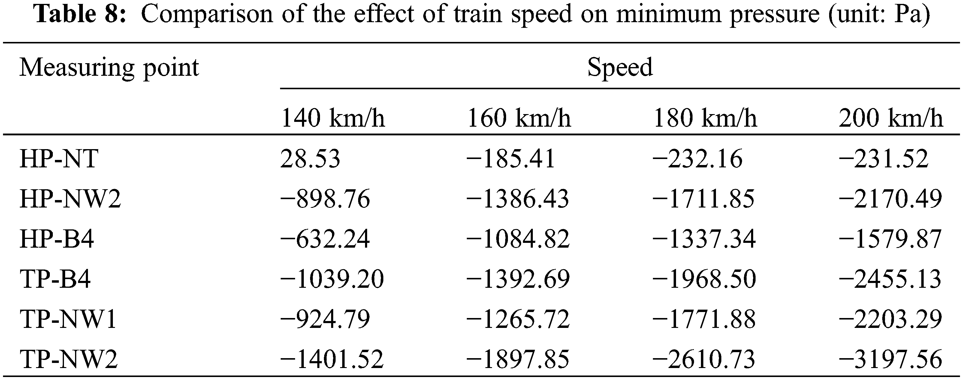
For the above typical measurement points, it can be found that the peak positive pressure of the head car at different speeds is proportional to the square of the velocity. The relationship between the maximum pressure Pmax (unit: Pa) at the measurement points of the head car, and the velocity V, was fitted, and the fitted function coefficients as shown in Table 9 were obtained by fitting by Eq. (3). These R2 values of the fitted equations for the peak positive pressure at the nose and body of the head car in the table are above 0.99, which indicates the reasonableness of the fitted equations.
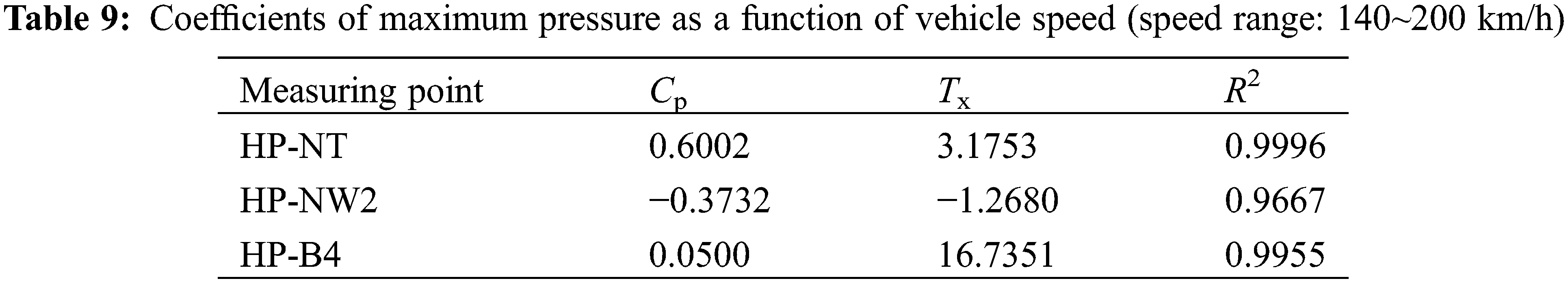
where, Cp is the pressure coefficient of the measuring points when the train is running in the open air.
This study investigates the aerodynamic characteristics of urban rail trains passing through tunnels at different speeds. It analyzes how running speed affects train aerodynamic force and surface pressure, and provides surface pressure characteristics at typical positions. The study derives relationship equations for train aerodynamic drag, maximum surface pressure on the head car, and running speed. The main conclusions are as follows:
1. At 160 km/h, the train’s peak aerodynamic drag increases by about 2.89 times, with the head car’s peak drag increasing by 3.62 times, and the tail car by 3.27 times. The average drag increases by 1.56 times, with the tail car seeing the largest increase (1.84 times), followed by the head car (1.74 times). Compared to 140 km/h, the whole car drag increases by 32.16%, 61.60%, and 99.66%, at speeds of 160, 180, and 200 km/h, respectively.
2. The head car hood, being on the windward side, has the largest positive pressure amplitude, followed by the nose and the driver’s room windshield. In the same body section, the top pressure is larger than in other places, and symmetrical positions have similar pressure curves. The tail car’s driver’s room windshield has the highest pressure, and the side windows’ negative pressure peak is the largest.
3. As speed increases, the positive and negative pressure amplitudes at measurement points increase, but the minimum pressure at the head car nose tip, and the maximum pressure at the tail car change insignificantly. Compared to 140 km/h, the positive pressure amplitude at the nose tip increases by 29.85%, 62.77%, and 102.34%, and the negative pressure amplitude at the tail car window increases by 35.41%, 86.28%, and 128.15% at speeds of 160, 180, and 200 km/h, respectively.
4. Train aerodynamic drag and maximum surface pressure on the head car are proportional to the square of the speed, with R² values of the fitted equations for drag and peak positive pressure all being greater than 0.99.
Due to the limitations of computational resources, only the standard k-ε model is used for numerical calculations in this paper. Compared with other models, the standard k-ε model has many shortcomings in predicting the characteristics of complex flow fields. More improved models, such as LES, RANS-LES, and other improved k-ε models, will be used in subsequent studies.
Acknowledgement: None.
Funding Statement: This study is supported by the Beijing Postdoctoral Research Foundation (No. 2023-ZZ-133), Scientific Research Foundation of Beijing Infrastructure Investment Co., Ltd. (No. 2023-ZB-03) and Fundamental Research Funds for the Central Universities (No. 2682023ZTPY036).
Author Contributions: Study conception and design: Haoran Meng, Tian Li; data collection: Haoran Meng, Xukui Shen; analysis and interpretation of results: Haoran Meng, Hong Zhang; draft manuscript preparation: Haoran Meng, Nianxun Li. All authors reviewed the results and approved the final version of the manuscript.
Availability of Data and Materials: The data presented in this study is available from the corresponding author, upon reasonable request. The data is not publicly available due to privacy.
Ethics Approval: Not applicable.
Conflicts of Interest: The authors declare no conflicts of interest to report regarding the present study.
References
1. Baron A, Mossi M, Sibilla S. The alleviation of the aerodynamic drag and wave effects of high-speed trains in very long tunnels. J Wind Eng Ind Aerodyn. 2001;89(5):365–401. [Google Scholar]
2. Baker C, Jordan S, Gilbert T, Quinn A, Sterling M, Johnson T, et al. Transient aerodynamic pressures and forces on trackside and overhead structures due to passing trains. Part 1: model-scale experiments; Part 2: standards applications. Proc Inst Mech Eng Part F: J Rail Rapid Transit. 2014;228(1):37–70. [Google Scholar]
3. Morden JA, Hemida H, Baker CJ. Comparison of RANS and detached eddy simulation results to wind-tunnel data for the surface pressures upon a class 43 high-speed train. J Fluid Eng. 2015;137(4):041108. [Google Scholar]
4. Gallagher M, Morden J, Baker C, Soper D, Quinn A, Hemida H, et al. Trains in crosswinds-comparison of full-scale on-train measurements, physical model tests and CFD calculations. J Wind Eng Ind Aerodynamics. 2018;175:428–44. [Google Scholar]
5. Khayrullina A, Blocken B, Janssen W, Straathof J. CFD simulation of train aerodynamics: train-induced wind conditions at an underground railroad passenger platform. J Wind Eng Ind Aerodynamics. 2015;139:100–10. [Google Scholar]
6. Li T, Li Y, Wei L, Zhang J. Study on lateral vibration of tail coach for high-speed train under unsteady aerodynamic loads. Vibration. 2023;6(4):1048–59. doi:10.3390/vibration6040061. [Google Scholar] [CrossRef]
7. Gilbert T, Baker C, Quinn A. Gusts caused by high-speed trains in confined spaces and tunnels. J Wind Eng Ind Aerodynamics. 2013;121(1):39–48. doi:10.1016/j.jweia.2013.07.015. [Google Scholar] [CrossRef]
8. Du J, Fang Q, Wang J, Wang G. Influences of high-speed train speed on tunnel aerodynamic pressures. Appl Sci. 2021;12(1):303. doi:10.3390/app12010303. [Google Scholar] [CrossRef]
9. Munoz-Paniagua J, García J, Crespo A. Genetically aerodynamic optimization of the nose shape of a high-speed train entering a tunnel. J Wind Eng Ind Aerodyn. 2014;130(5):48–61. doi:10.1016/j.jweia.2014.03.005. [Google Scholar] [CrossRef]
10. Choi JK, Kim KH. Effects of nose shape and tunnel cross-sectional area on aerodynamic drag of train traveling in tunnels. Tunn Undergr Space Technol Incorporating Trenchless Technol Res. 2014;41:62–73. doi:10.1016/j.tust.2013.11.012. [Google Scholar] [CrossRef]
11. Ricco P, Baron A, Molteni P. Nature of pressure waves induced by a high-speed train travelling through a tunnel. J Wind Eng Ind Aerodyn. 2007;95(8):781–808. [Google Scholar]
12. Liu DX, Jiang YN, Yang MZ. Study on tunnel aerodynamic of subway train during acceleration. J Railw Sci Eng. 2018;15(1):178–87. [Google Scholar]
13. Ogawa T, Fujii K. Numerical investigation of three-dimensional compressible flows induced by a train moving into a tunnel. Comput Fluids. 1997;26(6):565–85. [Google Scholar]
14. Howe M, Iida M, Fukuda T, Maeda T. Theoretical and experimental investigation of the compression wave generated by a train entering a tunnel with a flared portal. J Fluid Mech. 2000;425:111–32. [Google Scholar]
15. Miyachi T, Saito S, Fukuda T, Sakuma Y, Ozawa S, Arai T, et al. Propagation characteristics of tunnel compression waves with multiple peaks in the waveform of the pressure gradient: part 1: field measurements and mathematical model. Proc Inst Mech Eng Part F: J Rail Rapid Transit. 2016;230(4):1297–308. [Google Scholar]
16. Song JH, Guo DL, Yang GW, Yang QS. Experimental investigation on the aerodynamics of tunnel-passing for high speed train with a moving model rig. J Exp Fluid Mech. 2017;31(5):39–45. [Google Scholar]
17. Negri S, Tomasini G, Schito P, Rocchi D. Full scale experimental tests to evaluate the train slipstream in tunnels. J Wind Eng Ind Aerodyn. 2023;240(5):105514. doi:10.1016/j.jweia.2023.105514. [Google Scholar] [CrossRef]
18. Zhang L, Yang MZ, Niu JQ, Liang XF, Zhang J. Moving model tests on transient pressure and micro-pressure wave distribution induced by train passing through tunnel. J Wind Eng Ind Aerodyn. 2019;191(5):1–21. doi:10.1016/j.jweia.2019.05.006. [Google Scholar] [CrossRef]
19. Chen G, Li XB, Liu Z, Zhou D, Wang Z, Liang XF, et al. Dynamic analysis of the effect of nose length on train aerodynamic performance. J Wind Eng Ind Aerodyn. 2019;184(6):198–208. doi:10.1016/j.jweia.2018.11.021. [Google Scholar] [CrossRef]
20. Li T, Dai Z, Zhang W. Effect of RANS model on the aerodynamic characteristics of a train in crosswinds using DDES. Comput Model Eng Sci. 2020;122(2):555–70. doi:10.32604/cmes.2020.08101. [Google Scholar] [CrossRef]
21. Luo C, Zhou D, Chen G, Krajnovic S, Sheridan J. Aerodynamic effects as a maglev train passes through a noise barrier. Flow, Turbul Combust. 2020;105(3):761–85. doi:10.1007/s10494-020-00162-w. [Google Scholar] [CrossRef]
22. Chode K, Viswanathan H, Chow K, Reese H. Investigating the aerodynamic drag and noise characteristics of a standard squareback vehicle with inclined side-view mirror configurations using a hybrid computational aeroacoustics (CAA) approach. Phys Fluids. 2023;35(7):35–7. doi:10.1063/5.0156111. [Google Scholar] [CrossRef]
23. Rabani M, Faghih AK. Numerical analysis of airflow around a passenger train entering the tunnel. Tunnelling Undergr Space Technol. 2015;45(5):203–13. doi:10.1016/j.tust.2014.10.005. [Google Scholar] [CrossRef]
24. Zhou MM, Liu TH, Xia YT, Li WH, Chen ZW. Comparative investigations of pressure waves induced by trains passing through a tunnel with different speed modes. J Central South Univ. 2022;29(8):2639–53. doi:10.1007/s11771-022-5098-2. [Google Scholar] [CrossRef]
25. Heine D, Ehrenfried K, Heine G, Huntgeburth S. Experimental and theoretical study of the pressure wave generation in railway tunnels with vented tunnel portals. J Wind Eng Ind Aerodyn. 2018;176:290–300. doi:10.1016/j.jweia.2018.03.020. [Google Scholar] [CrossRef]
26. Liu T, Jiang Z, Chen X, Zhang J, Liang X. Wave effects in a realistic tunnel induced by the passage of high-speed trains. Tunnelling Undergr Space Technol. 2019;86:224–35. doi:10.1016/j.tust.2019.01.023. [Google Scholar] [CrossRef]
27. Chen T, Lee Y, Hsu CC. Investigations of piston-effect and jet fan-effect in model vehicle tunnels. J Wind Eng Ind Aerodyn. 1998;73(2):99–110. doi:10.1016/S0167-6105(97)00281-X. [Google Scholar] [CrossRef]
28. Mok J, Yoo J. Numerical study on high speed train and tunnel hood interaction. J Wind Eng Ind Aerodyn. 2001;89(1):17–29. doi:10.1016/S0167-6105(00)00021-0. [Google Scholar] [CrossRef]
29. Srivastava S, Sivasankar G, Dua G. A review of research into aerodynamic concepts for high speed trains in tunnels and open air and the air-tightness requirements for passenger comfort. Proc Inst Mech Eng Part F: J Rail Rapid Transit. 2022;236(9):1011–25. doi:10.1177/09544097211072973. [Google Scholar] [CrossRef]
30. Xiong X, Zhu L, Zhang J, Li A, Li X, Tang M. Field measurements of the interior and exterior aerodynamic pressure induced by a metro train passing through a tunnel. Sustain Cities Soc. 2020;53(6):101928. doi:10.1016/j.scs.2019.101928. [Google Scholar] [CrossRef]
31. Sun Z, Yang G, Zhu L. Study on the critical diameter of the subway tunnel based on the pressure variation. Sci China Technol Sci. 2014;57(10):2037–43. doi:10.1007/s11431-014-5664-4. [Google Scholar] [CrossRef]
32. Yang X, Shou A, Zhang R, Quan J, Li X, Niu J. Numerical study on transient aerodynamic behaviors in a subway tunnel caused by a metro train running between adjacent platforms. Tunnelling Undergr Space Technol. 2021;117(6–7):104152. doi:10.1016/j.tust.2021.104152. [Google Scholar] [CrossRef]
33. Wang J, Wan X, Wu J. Influence of tunnel lengths upon air pressure fluctuation in high speed railway tunnels. Mod Tunnelling Technol. 2008;45(6):1–4. [Google Scholar]
34. Li T, Qin D, Zhang J. Effect of RANS turbulence model on aerodynamic behavior of trains in crosswind. Chin J Mech Eng. 2019;32(1):1–12. doi:10.1186/s10033-019-0402-2. [Google Scholar] [CrossRef]
35. Zampieri A, Rocchi D, Schito P, Somaschini C. Numerical-experimental analysis of the slipstream produced by a high speed train. J Wind Eng Ind Aerodyn. 2020;196(5):104022. doi:10.1016/j.jweia.2019.104022. [Google Scholar] [CrossRef]
36. Ran T, Liang X, Xiong X. Study on sectional area of high-speed subway tunnel with speed of 140 km/h. J Cent South Univ (Sci Technol). 2019;50(10):2603–12 (In Chinese). [Google Scholar]
Cite This Article
 Copyright © 2025 The Author(s). Published by Tech Science Press.
This work is licensed under a Creative Commons Attribution 4.0 International License , which permits unrestricted use, distribution, and reproduction in any medium, provided the original work is properly cited.
 Downloads
 Citation Tools