Numerical Simulation of Gas-LiquId Flow in a Horizontal Elbow

1  Introduction

Gas-liquid flow (GLF) widely occurs in petroleum and natural gas engineering. Slug and annular flows are two common flow patterns [1] occurring at high gas and low liquid flow rates [2]. In slug flow, fluctuations in parameters such as velocity and pressure may affect the safe transportation of pipelines. In an annular flow, the liquid phase flows in the form of a liquid film on the pipe wall, the gas phase flows in the center of the pipe, and some of the liquid film flows in the form of droplets in the gas phase owing to the shear effect of the airflow. When an annular flow flows through an elbow, a secondary flow and flow separation occur, and changes in the flow parameters can cause corrosion and damage to the pipeline. Therefore, studying the slug and annular flow characteristics of elbows is crucial for designing and maintaining piping systems [3].

Several studies have been conducted on the properties of slugs and annular flow. Yin et al. [4] experimentally and numerically investigated the gas-liquid slug flow in a hilly terrain pipeline at low superficial liquid velocities and explained the evolutionary process of slug flow in a corrugated pipeline through pressure drop fluctuations, liquid-holding rates, and phase distributions. Widodo et al. [5] discussed the flow law of a 45° vertical–upward horizontal pipe. The frequency of the slug flow increased with gas velocity, whereas the pressure drop decreased. Akhlaghi et al. [6] studied the slug flow in a pipeline and observed that the SGV (superficial gas velocity) had a greater effect on the start position of the slug and the fully developed length of the slug than the SLV (superficial liquid velocity), and that an increase in the SLV decreased the slug length and liquid film thickness, whereas the liquid slug length and lateral slug velocity increased. Gourma et al. [7] numerically investigated the forces and loads of the slug flow in an elbow using a VOF (Volume of Fraction) model. Abdulkadir et al. [8] conducted studies on slug flow and reported that CFD (Computational Fluid Dynamics) simulations can predict the flow pattern before and after the elbow. Kesana et al. [9] and Parsi et al. [10] reported that the erosion rate of the slug flow increased with increasing grain size, SGV, and SLV. Al-Lababidi et al. [11,12] investigated the movement of sand particles in a slug flow in a pipe.

Researchers have also studied annular-flow liquid films in both vertical and horizontal tubes. Jing et al. [13] conducted experiments on oil–water flow in a pipeline with a 90° elbow and assessed the effect of the elbow on the stability of annular flow evolution by comparative analysis of the flow pattern and friction pressure gradient in the upstream and downstream sections; however, they lacked a detailed characterization of the distribution characteristics of the different phases in the pipeline cross-section. López et al. [14] conducted indoor experiments and numerical simulations of gas-liquid annular flow in a 180° elbow and described the effects of the radius of curvature and SGV on the behavior of the liquid film and the flow characteristics of the annular flow. Tkaczyk et al. [15] simulated gas-liquid annular flow in an elbow based on a modified fluid volume method using the finite volume method. Bandyopadhyay et al. [16] studied annular flow in four types of U-shaped elbows and compared the results calculated using FLUENT with the experimental results. Ribeiro et al. [17] investigated the droplet size in a two-phase horizontal annular flow at different gas-liquid ratios. The experimental results showed that the droplets enlarged after passing through the elbow. Abdulkadir et al. [18] experimentally investigated the liquid-film thickness distribution in a 180° reflux elbow. The experimental results revealed that, at higher liquid flow rates, the liquid film thickness in the inner part of the elbow was relatively high. Li et al. [19] experimentally investigated the effects of the superficial velocity on the slug and annular flow characteristics at micro-T junctions. Wu et al. [20] investigated the hydrodynamic characteristics of an annular flow in a 90° elbow using a VOF model.

Horizontal 90° elbows are widely used in natural-gas-gathering pipelines and constitute one of the most severely eroded and worn locations in pipeline systems. The erosion rate of the elbow section was much higher than that of the straight pipe section, with a magnitude approximately 50 times that of the straight pipe section. The elbow section is the weakest link in a mixed-flow pipeline and is the most susceptible to erosion and damage. Therefore, studying the flow characteristics of the slug and annular flows in the elbow section is helpful for studying elbow erosion and erosion resistance. Therefore, CFD numerical simulation methods were used to study the phase, pressure, and velocity distributions inside pipelines under different velocity conditions as well as the influence of elbows on the slug and annular flow laws. The aim of this research is to provide a more accurate and comprehensive description of the characteristic parameters of slug and annular flow at elbows and to provide theoretical guidance for the study of erosion mechanisms, elbow design, and protection of elbows to provide a theoretical basis and assistance for the study of oil and gas mixed transportation technology and multiphase-flow elbow erosion and corrosion, ultimately ensuring the economic and safe production and operation of oil and gas fields.

2  Numerical Methods

2.1 Geometric Model

The simulated elbow was a 90° elbow, the pipe diameter D = 50 mm, and the bending ratio R/D = 5, which was the same as that in the experiment. Because the numerical simulation in this study involves transient calculation, to ensure the full development of the GLF in the pipe while considering the calculation consumption of the model, the lengths of the inlet of the elbow is 100D, the length of the outlet is 30D, the length of the inlet of the elbow is 30D, and the length of the outlet is 20D. The geometric model is shown in Fig. 1.

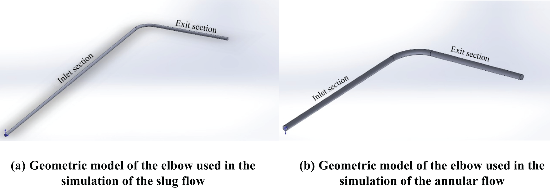
Figure 1: Geometric model of a 90° horizontal elbow

2.2 Mesh Generation

A quadrilateral mesh was adopted to divide the faces of the elbows, an O-block was used at the entrances and exits, and the grid density near the boundary was relatively high. After meshing, the hexahedral structured mesh is converted into an unstructured mesh in ICEM and exported for storage. To check the grid dependence, different numbers of grids were generated, and the grid independence verification results are shown in Table 1. The number of grid nodes of the slug and annular flows in this study were 463,375 and 193,775, respectively; the numbers of grids were 439,680 and 183,680, respectively; and the mesh quality was 0.642. The details of the meshing division are shown in Fig. 2.

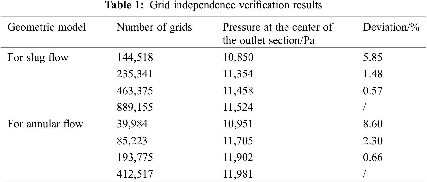
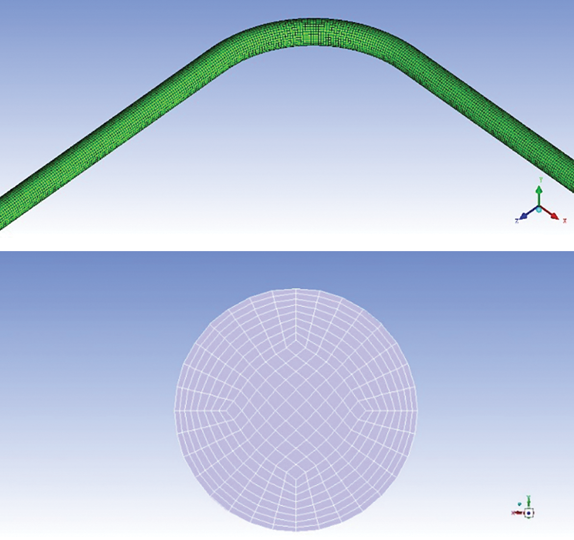
Figure 2: Elbow mesh division

2.3 Physical Model

The flow of the GLF is modeled by a numerical solution of a set of equations describing the broadest case of medium movement. The numerical models (including the mass and momentum equations) of the GLF are as follows [21]:

(1) Continuity equation

∂ρ∂t+∇⋅(ρul→)=0 (1)

where ρ=ρlαl+(1−αl)ρg , ρl and ρg represent the density of liquid and gas, αl represents the phase volume fraction of liquid, u→ is the velocity vector, and t is the time.

(2) Momentum conservation equation

∂(ρui)∂t+∂(ρuiuj)∂xj=−∂p∂xi+∂τij∂xj+∂τijRe∂xj+ρgi (2)

where p, ρ, τij and τijRe represent the static pressure, the density of a combined phase, the stress tensor, and the turbulent stress, respectively. gi represents the gravitational volume force in the i-direction.

(3) Turbulence model

The standard k–ε turbulence model is used in this study, and the k and ε equations are expressed as follows:

∂(pk)∂t+∂(pkui)∂xi=∂∂xj[(μ+μtσk)∂k∂xj]+GK+Gb−pε−YM+Sk (3)

∂(pε)∂t+∂(pεui)∂xi=∂∂xj[(μ+μtσe)∂ε∂xj]+C1εεk(Gk+G3εGb)−C2εpε2k+Sε (4)

where YM is the diffusion loss, σk and σe are the Prandtl numbers of k and ε equations, respectively, and Sk and Sε are user-defined terms. Gk is the turbulent kinetic energy obtained from Gk=μtS2 . S is the coefficient of the stress tensor, which can be obtained using S=2Si,jSi,j . Gb is the turbulent kinetic energy generated by buoyancy, which can be obtained using Gb=−gμtρPrt∂p∂xi and Prt=0.85 . Si,j is the mean strain rate obtained via Si,j=12(∂uj∂xi+∂ui∂xj) . The coefficients C and η are obtained using C=max[0.43,ηη+5] , η=Skε .

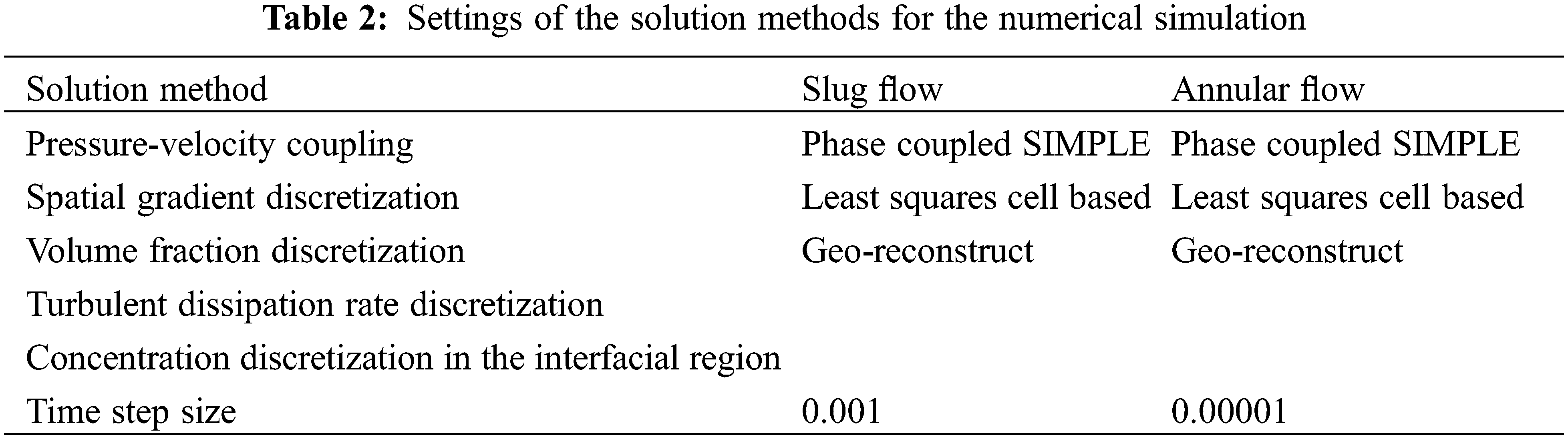
2.4 Numerical Simulation Solution Setting

The pressure-based unsteady state was chosen for the solution calculation, the Y-axis was set with a gravity of 9.81 m/s2, and the negative sign indicated that the gravity direction was along the negative direction of the Y-axis. The multifluid VOF model is activated, the explicit computation is selected, the Courant number is set to 0.25, the convergence condition is set to residuals of less than 10−5, and the turbulence model is selected to be the standard k–ε model. Air and water were used as primary and secondary phases, respectively. The inlet was divided into two parts in FLUENT: the slug-flow simulation inlet was layered with a height ratio of 0.5, and the annular-flow simulation inlet was divided into a small circle with a radius of 20 mm and a ring, with air flowing through the red channel and water flowing through the blue channel, as shown in Fig. 3. The inlet and outlet were set as the velocity and pressure outlet boundary conditions, respectively, and the wall adopted a no-slip wall boundary condition. The input GLF rate at the inlet needs to be recalculated according to the principle of mass flow conservation. For example, the value of the input flow rate at the liquid phase inlet is equal to the superficial flow rate of the liquid phase multiplied by the ratio of the cross-sectional area of the pipeline and the cross-sectional area of the liquid phase inlet. The input GLF rates for this slug flow simulation were twice the superficial flow rate, the input gas flow rate for the annular flow simulation was the value of the SGV divided by 0.64, the input liquid flow rate was the value of the SLV divided by 0.36, and the outlet pressures were all set to atmospheric pressure.

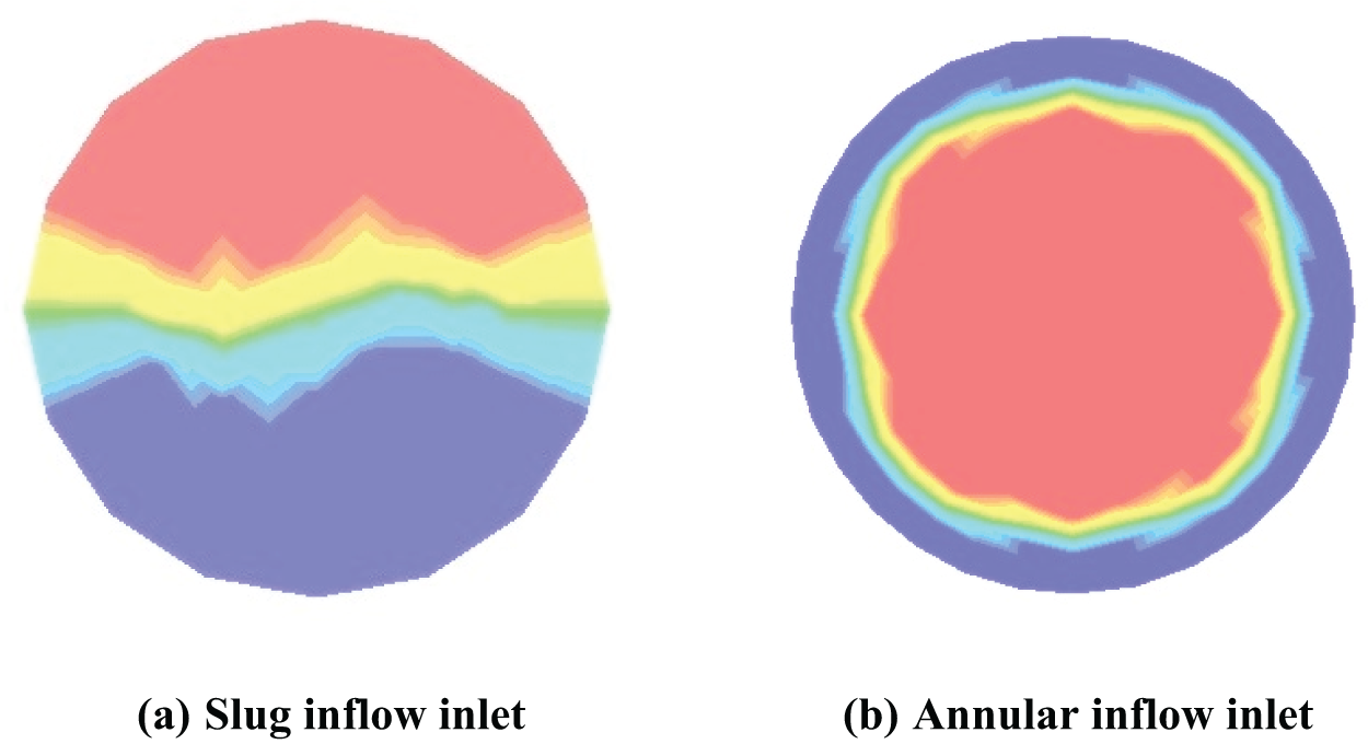
Figure 3: Inlet of gas-liquid two-phase

In FLUENT, for the transient numerical simulation calculation of multiphase flow under the condition of convergence, to improve accuracy, the numerical simulation solution settings in this study are listed in Table 2.

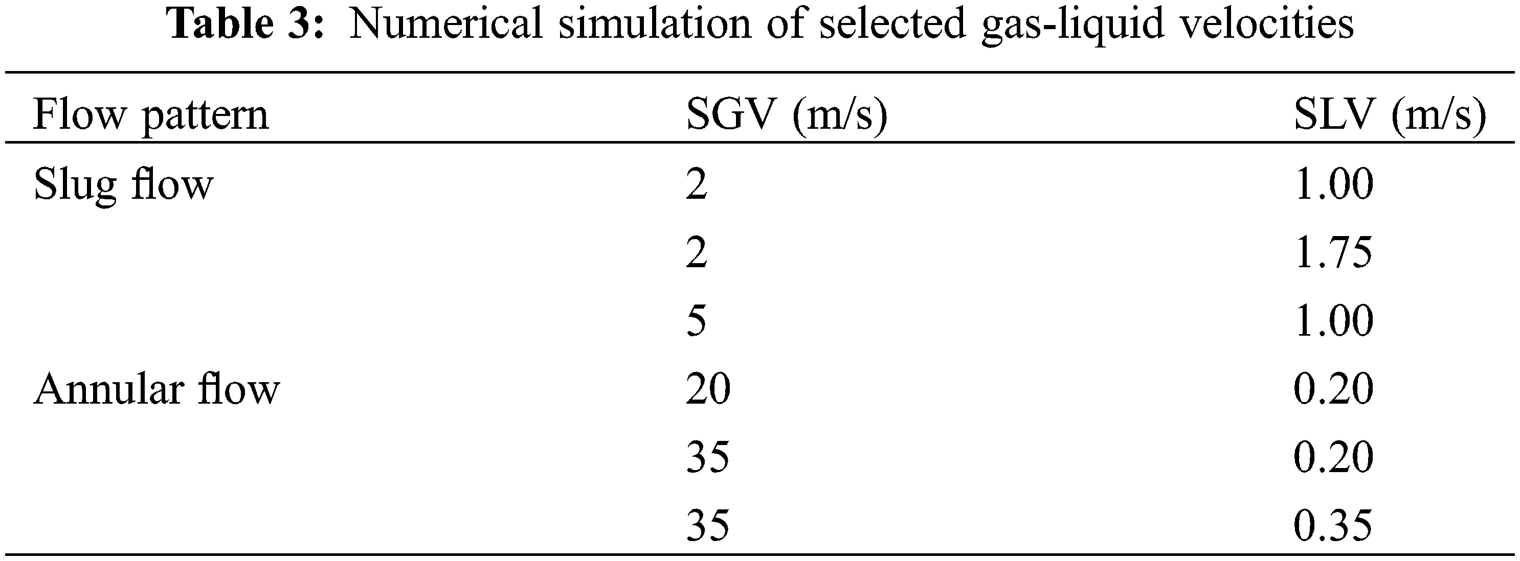
2.5 Determination of the Simulated GLF Rate

Numerical simulation research is an expansion and supplementation of experimental research. This study conducted numerical simulations under some experimental research conditions, and the conditions for the GLF rate are listed in Table 3.

2.6 Model Validation

Using the experimental conditions of a superficial gas velocity of 35 m/s and a superficial liquid velocity of 0.20 m/s as examples, the gas content at the inlet and outlet of the bent pipe was obtained through WMS processing, and the simulation results based on the established model were compared with the experimental data (as shown in Fig. 4). Because the length of the experimental pipeline is longer than that of the model, as well as because of factors such as fluctuations in the amount of incoming gas and liquid, the simulation results have slight deviations from the experimental results, but are generally close, and the trend of change is the same.

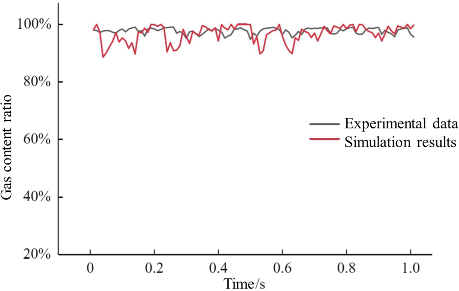
Figure 4: Comparison between experimental and simulated value of air content at the outlet of 90° elbow

3  Results and Discussion

3.1 Simulation Results of Slug Flow in the Elbow Section

Transient numerical simulations were performed for three sets of conditions with superficial gas and liquid velocities of 2 and 1 m/s, 2 and 1.75 m/s, and 5 and 1 m/s, respectively, for the slug flow. Pressure cloud diagrams, liquid velocity cloud diagrams, and vector diagrams corresponding to the liquid slug in the pipe under different velocities in the horizontal pipe slug flow were obtained to analyze the flow characteristics of the slug flow in the horizontal pipe, such as pressure and liquid velocity, and to study the effects of changes in the GLF velocity.

3.1.1 Pressure Cloud Diagram

The results of the transient simulation of the three sets of slug flows were processed via CFD-Post to obtain the pressure cloud diagrams in the elbow at different velocities (Fig. 5).

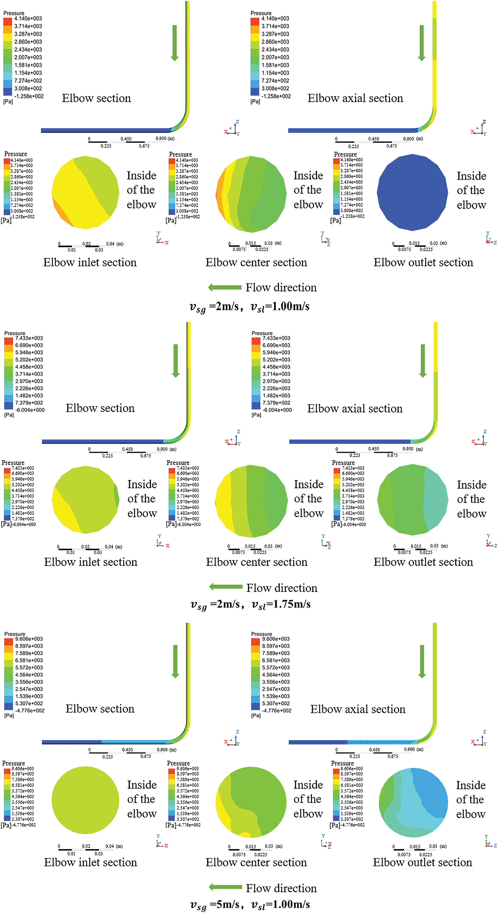
Figure 5: Pressure diagrams of slug flow in elbow

As shown in Fig. 5, the pressure of the entire pipeline decreased because of the energy consumption of the fluid during the flow process. In the pressure cloud diagrams of the axial and radial sections, the pressure in the elbow was uneven. The pressure on the outer side of the elbow was greater than that on the inner side and gradually decreased from the outer to the inner part of the elbow. A centrifugal force inside the elbow causes air bubbles in the liquid slug to flow on the inner side of the elbow, resulting in a stepped radial pressure distribution in the elbow.

3.1.2 Liquid Velocity Cloud Diagram and Vector Diagram

The results of the transient simulation of the three sets of slug flows were processed using CFD-Post to obtain the liquid velocity cloud diagrams (Fig. 6).

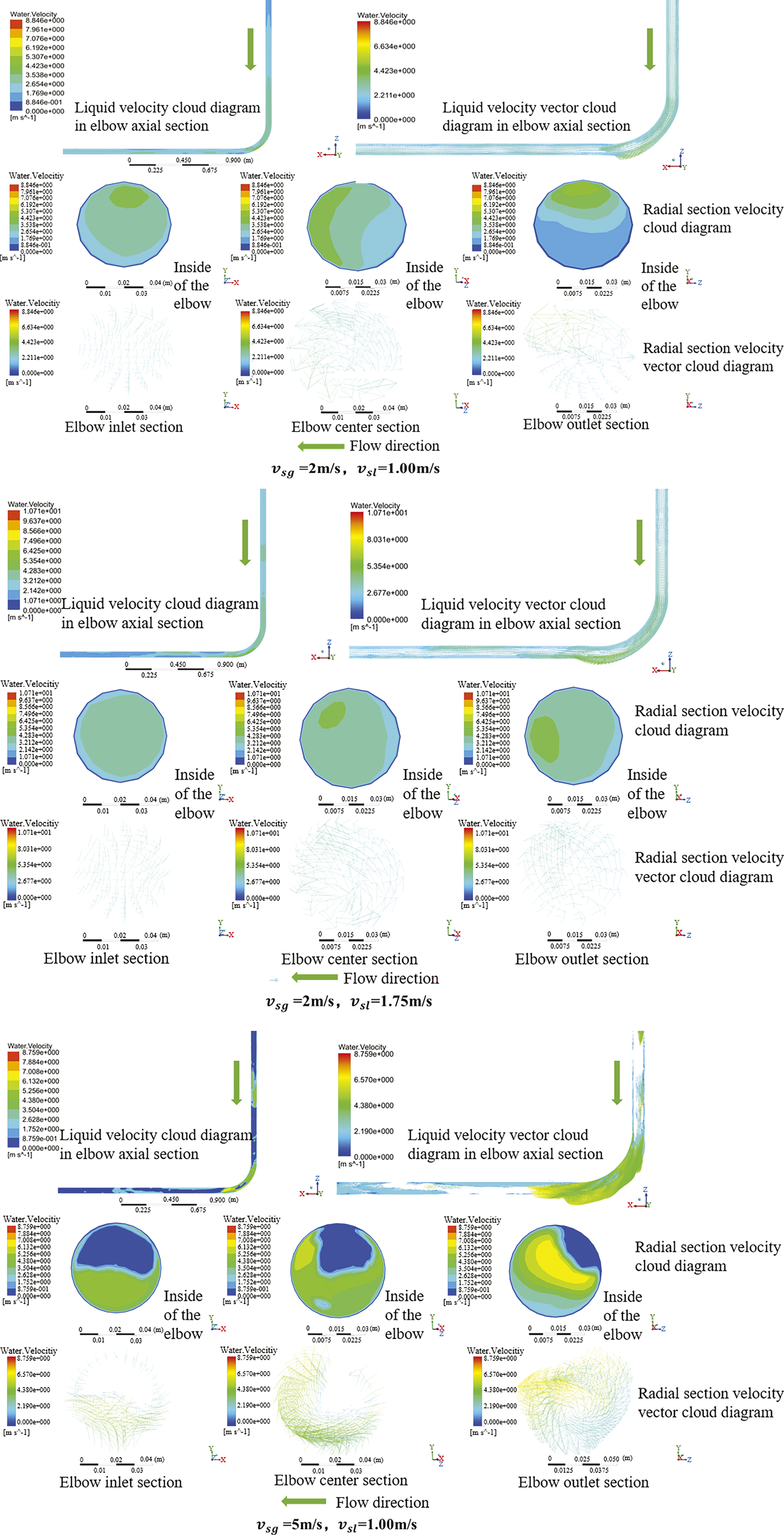
Figure 6: Liquid velocity cloud and vector diagrams of slug flow in elbows

According to the velocity cloud diagram of the axial section shown in Fig. 6, the liquid velocity in the liquid slug region is the highest. Because of the centrifugal force, the liquid velocity inside the elbow was uneven, and the liquid velocity on the outer side was larger than that on the inner side. As SLV and SGV increased, the liquid velocity in the slug flow also increased.

According to the axial and radial section velocity vector diagrams, the liquid was biased toward the outside of the elbow flow owing to the centrifugal force of the elbow. The secondary flow at the center and outlet sections of the elbow formed vortices; however, as the GLF velocity increased, the secondary flow weakened.

3.2 Simulation Results of Annular Flow in an Elbow

Transient simulations were conducted for three sets of conditions with superficial gas and liquid velocities of 20 and 0.20 m/s, 35 and 0.20 m/s, and 35 and 0.35 m/s, respectively, for annular flow. Pressure distribution cloud diagrams, liquid velocity cloud diagrams, and vector diagrams corresponding to different flow velocities of the elbow annular flow were obtained to analyze the effects of varying the gas and liquid flow velocities on the flow characteristics of the annular flow.

3.2.1 Pressure Cloud Diagram

The results of the three sets of annular flow transient simulations were processed using CFD-Post to obtain the pressure cloud diagrams of the annular flow (Fig. 7).

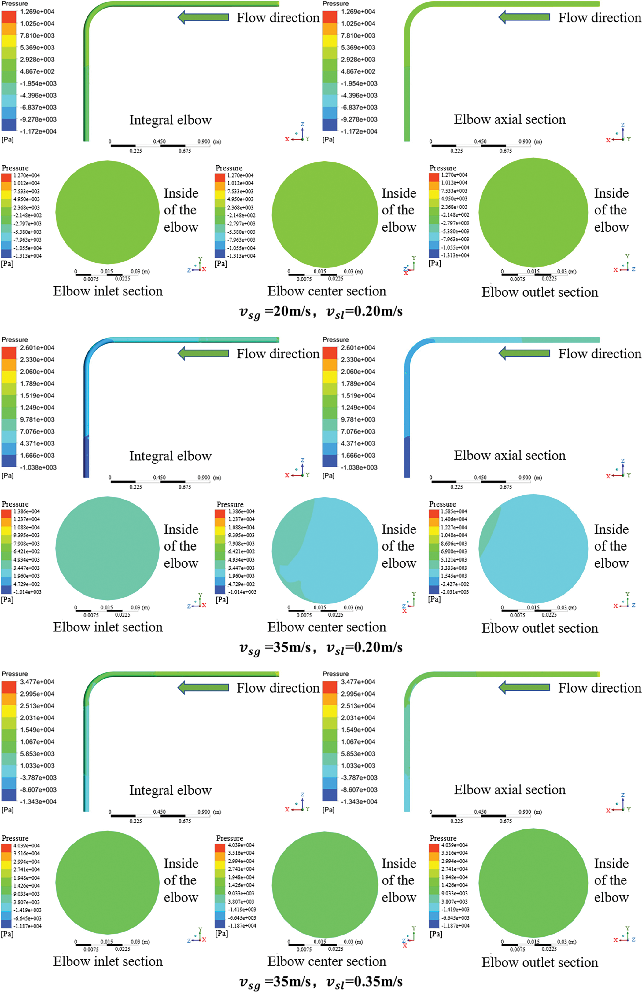
Figure 7: Pressure nephogram of annular flow in an elbow

As shown in Fig. 7, the pressure of the entire pipeline of the elbow annular flow shows a decreasing trend; although the pressure of the inner elbow is lower than that of the outer elbow, the difference in the inner and outer pressures is not significant. This is mainly because although the liquid film distribution on the inner and outer pipe walls of the annular flow in the elbow is uneven, it can lead to differences in the inner and outer pressures of the elbow; however, this difference is not obvious at high gas velocities. A comparison of the pressure distributions in the elbow at different GLF rates revealed that the pressure at different positions on the elbow increased with increasing SLV and SGV; however, a change in the SGV had a greater effect on the elbow pressure.

3.2.2 Liquid Velocity Cloud Diagram and Vector Diagram

The results of the three sets of annular flow transient simulations were processed using CFD-Post to obtain the liquid velocity cloud diagrams and vector diagrams of the annular flow (Fig. 8).

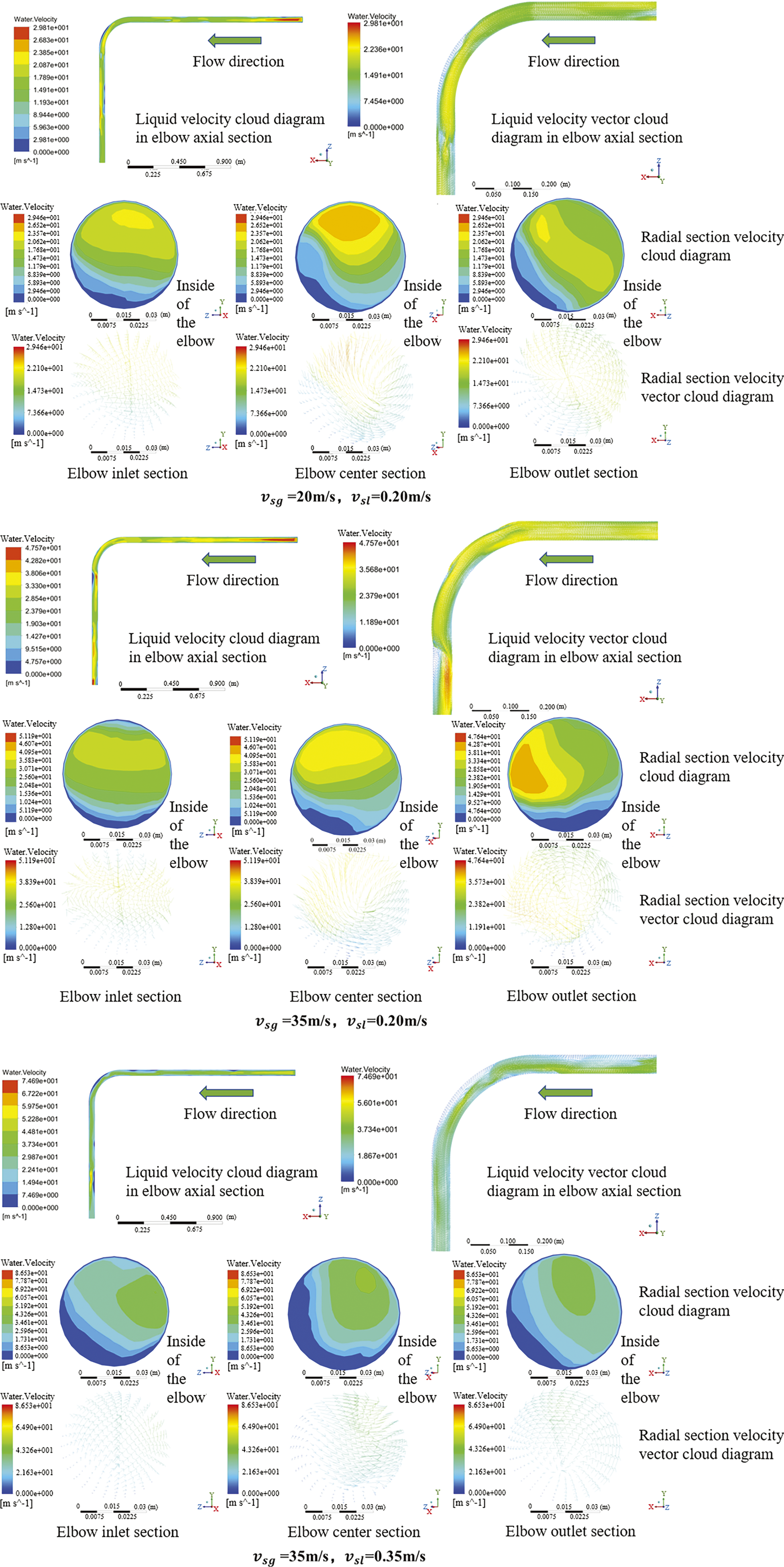
Figure 8: Liquid velocity cloud and vector diagram of annular flow in an elbow

According to the liquid velocity cloud diagrams of the axial and radial sections in shown Fig. 8, the distribution of the annular flow liquid velocity inside the elbow was uneven, and the velocity in the main liquid film area was the smallest. With increasing SLV, the annular flow velocity inside the elbow increased; however, an increase in the liquid film outside the elbow decreased the liquid velocity outside the elbow. As the SGV increased, the annular liquid flow rate in the elbow increased, the liquid film outside the elbow decreased, and the liquid flow rate outside the elbow increased.

4  Conclusion

In this study, the multifluid VOF model was selected in FLUENT for the numerical simulation of the elbow section. The flow fields corresponding to different calculation conditions of the slug and annular flow in the elbow section were obtained to analyze the effects of gas and liquid flow rate changes.

(1) The bubbles in the slug flow liquid slug of the elbow move inside the elbow, and the pressure in the entire pipeline decreases. The pressure inside the elbow was lower than that outside. The liquid velocity inside the elbow was uneven, and the liquid velocity outside the elbow was greater than that inside the elbow. There is a secondary flow in the elbow section, which has a small impact on the inlet of the elbow and a large impact on the center and downstream of the bend pipe.

(2) The liquid film of annular flow at outside the elbow was thicker than that inside the elbow, the pressure of the entire pipeline showed a downward trend, the pressure on the outside of the elbow was greater than that on the inside, the liquid flow velocity in the elbow was uneven, and the liquid velocity in the main liquid film area was the lowest. With increasing SLV and SGV, the pressure and liquid flow velocity at different positions in the elbow increased, and the secondary flow in the elbow weakened.

The above conclusion accurately and comprehensively describes the characteristic parameters of slug and annular flows at elbows and provides theoretical guidance for the study of erosion mechanisms, elbow design, and elbow protection. It also provides a theoretical basis and assistance for research on oil and gas mixed transportation technology and multiphase-flow elbow erosion and corrosion, ultimately ensuring economic and safe production and operation of oil and gas fields.

Acknowledgement: Thanks to the State Key Laboratory of Low Carbon Catalysis and Carbon Dioxide Utilization for supporting this work.

Funding Statement: This work was supported by the Ministry of Industry and Information Technology High Tech Ship Special Project (Grant No. CBG3N21-2-6).

Author Contributions: The authors confirm contribution to the paper as follows: study conception and design: Lihui Ma, Wei Li; data collection: Yuanyuan Wang, Pan Zhang; analysis and interpretation of results: Lina Wang, Xinying Liu, Xuewen Cao; draft manuscript preparation: Lihui Ma, Meiqin Dong, Jiang Bian. All authors reviewed the results and approved the final version of the manuscript.

Availability of Data and Materials: The datasets generated and/or analyzed during the current study are available from the corresponding author on reasonable request.

Ethics Approval: Not applicable.

Conflicts of Interest: The authors declare no conflicts of interest to report regarding the present study.

References

1. Dong C, Lu L, Wang X. Experimental investigation on non-boiling heat transfer of two-component air-oil and air-water slug flow in horizontal pipes. Int J Multiphase Flow. 2019;119(7):119–41. doi:10.1016/j.ijmultiphaseflow.2019.07.004. [Google Scholar] [CrossRef]

2. Fan W, Cherdantsev AV, Anglart H. Experimental and numerical study of formation and development of disturbance waves in annular gas-liquid flow. Energy. 2020;207:118309. doi:10.1016/j.energy.2020.118309. [Google Scholar] [CrossRef]

3. Zhao X, Cao X, Xie Z, Cao H, Wu C, Bian J. Numerical study on the particle erosion of elbows mounted in series in the gas-solid flow. J Nat Gas Sci Eng. 2022;207(6):104423. doi:10.1016/j.jngse.2022.104423. [Google Scholar] [CrossRef]

4. Yin P, Cao X, Li Y, Yang W, Bian J. Experimental and numerical investigation on slug initiation and initial development behavior in hilly-terrain pipeline at a low superficial liquid velocity. Int J Multiphase Flow. 2018;101(5):S0301932217303919–96. doi:10.1016/j.ijmultiphaseflow.2018.01.004. [Google Scholar] [CrossRef]

5. Widodo A, Awaluddin S. Flow characteristic of horizontal-vertical upward air-water with 45° elbow. IOP Conf Ser: Mater Sci Eng. 2019;494:012031. doi:10.1088/1757-899X/494/1/012031. [Google Scholar] [CrossRef]

6. Akhlaghi M, Taherkhani M, Nouri NM. Study of intermittent flow characteristics experimentally and numerically in a horizontal pipeline. J Nat Gas Sci Eng. 2020;79(1):103326. doi:10.1016/j.jngse.2020.103326. [Google Scholar] [CrossRef]

7. Gourma M, Verdin PG. Nature and magnitude of operating forces in a horizontal bend conveying gas-liquid slug flows. J Pet Sci Eng. 2020;190(333):107062. doi:10.1016/j.petrol.2020.107062. [Google Scholar] [CrossRef]

8. Abdulkadir M, Hernandez-Perez V, Lo S, Lowndes IS, Azzopardi B. Comparison of experimental and computational fluid dynamics (CFD) studies of slug flow in a vertical 90° bend. J Comput Multiph Flows. 2013;5(4):265–81. doi:10.1260/1757-482X.5.4.265. [Google Scholar] [CrossRef]

9. Kesana N, Throneberry JM, McLaury B, Shirazi S, Rybicki E. Effect of particle size and liquid viscosity on erosion annular and slug flow. J Energy Resour Technol. 2014;136(1):50. doi:10.1115/1.4024857. [Google Scholar] [CrossRef]

10. Parsi M, Vieira RE, Kesana N, McLaury B, Shirazi S. Ultrasonic measurements of sand particle erosion in gas dominant multiphase churn flow in vertical pipes. Wear. 2015;329(1):401–13. doi:10.1016/j.wear.2015.03.013. [Google Scholar] [CrossRef]

11. Al-Lababidi S, Yan W, Yeung H. Sand transportations and deposition characteristics in multiphase flows in pipelines. J Energy Resour Technol. 2012;134(3):034501. doi:10.1115/1.4006433. [Google Scholar] [CrossRef]

12. Pedinotti S, Mariotti G, Banerjee S. Direct numerical simulation of particle behaviour in the wall region of turbulent flows in horizontal channels. Int J Multiphase Flow. 1992;18(6):927–41. doi:10.1016/0301-9322(92)90068-R. [Google Scholar] [CrossRef]

13. Jing J, Yin X, Mastobaev BN, Valeev A, Sun J, Wang S, et al. Experimental study on highly viscous oil-water annular flow in a horizontal pipe with 90° elbow. Int J Multiphase Flow. 2020;135:103499. doi:10.1016/j.ijmultiphaseflow.2020.103499. [Google Scholar] [CrossRef]

14. López J, Ratkovich N, Pereyra E. Analysis of two-phase air-water annular flow in U-bends. Heliyon. 2020;6(12):e05818. doi:10.1016/j.heliyon.2020.e05818. [Google Scholar] [PubMed] [CrossRef]

15. Tkaczyk P. CFD simulation of annular flows through bends. Nottingham: University of Nottingham; 2011. [Google Scholar]

16. Bandyopadhyay TK, Ghosh T, Das SK. Water and air-water flow through U-bends—experiments and CFD analysis. In: AIP Conference, 2010; West Bengal, India, American Institute of Physics; p. 110–5. doi:10.1063/1.3516285. [Google Scholar] [CrossRef]

17. Ribeiro AM, Bott TR, Jepson DM. The influence of a bend on drop sizes in horizontal annular two-phase flow. Int J Multiphase Flow. 2001;27(4):721–8. doi:10.1016/S0301-9322(00)00038-0. [Google Scholar] [CrossRef]

18. Abdulkadir M, Azzi A, Zhao D, Lowndes IS, Azzopardi B. Liquid film thickness behaviour within a large diameter vertical 180° return bend. Chem Eng Sci. 2014;107(9):137–48. doi:10.1016/j.ces.2013.12.009. [Google Scholar] [CrossRef]

19. Li HW, Li JW, Zhou YL, Liu B, Sun B, Yang D, et al. Phase split characteristics of slug and annular flow in a dividing micro-T-junction. Exp Therm Fluid Sci. 2017;80:244–58. doi:10.1016/j.expthermflusci.2016.08.024. [Google Scholar] [CrossRef]

20. Wu J, Jiang W, Liu Y, He Y, Chen J, Qiao L, et al. Study on hydrodynamic characteristics of oil-water annular flow in 90 degrees elbow. Chem Eng Res Des. 2020;153(6):443–51. doi:10.1016/j.cherd.2019.11.013. [Google Scholar] [CrossRef]

21. Doroshenko Y, Doroshenko J, Zapukhliak V, Poberezhny L, Maruschak P. Modeling computational fluid dynamics of multiphase flows in elbow and T-junction of the main gas pipeline. Transport. 2019;34(1):19–29. doi:10.3846/transport.2019.7441. [Google Scholar] [CrossRef]