
 Submit a Paper
 Propose a Special lssue
 Open Access
ARTICLE

Numerical Investigation of Wind Resistance in Inland River Low-Emission Ships
1 School of Mechanical and Electrical Engineering, Jining University, Qufu, 273155, China
2 Wuhan University of Technology Ship Cruise Center, Wuhan, 430063, China
3 Guangzhou Haige Communications Group Incorporated Company, Guangzhou, 510663, China
4 Shandong Xinneng Ship Technology Co., Jining, 277605, China
* Corresponding Author: Jichao Li. Email:
Fluid Dynamics & Materials Processing 2025, 21(11), 2721-2740. https://doi.org/10.32604/fdmp.2025.068889
Received 09 June 2025; Accepted 28 September 2025; Issue published 01 December 2025
 View Full Text
 Download PDF
Abstract
To enhance the navigation efficiency of inland new-energy ships and reduce energy consumption and emissions, this study investigates wind load coefficients under 13 conditions, combining a wind speed of 2.0 m/s with wind direction angles ranging from 0° to 180° in 15° increments. Using Computational Fluid Dynamics (CFD) simulations, the wind load is decomposed into along-course (CX) and transverse (CY) components, and their variation with wind direction is systematically analyzed. Results show that CX is maximal under headwind (0°), decreases approximately following a cosine trend, and reaches its most negative value under tailwind (180°). CY peaks at crosswind (90°) and exhibits an overall sinusoidal distribution. Certain wind directions produce a compound effect on the hull, particularly when the crosswind angle approaches 90°. Flow analysis reveals that wind generates a high-pressure zone on the windward side and a low-pressure vortex region on the leeward side, inducing unstable forces and increasing energy consumption. Based on the wind pressure distribution, a targeted structural optimization is proposed to mitigate high-pressure resistance. These findings provide a theoretical basis for hull form optimization and energy-efficient ship design.Keywords
1.1 Research Background and Significance
Green ships have great development prospects. They refer to the use of high-tech, energy-saving and environmentally friendly materials and manufacturing equipment in the design, manufacturing and operation of ships, and the integration of environmental protection concepts. Resource utilization and potential environmental impacts during shipbuilding are fully considered, with advanced process technologies applied to minimize resource waste and environmental pollution while enhancing the functional performance of ships to meet technical requirements. Liquefied natural gas (LNG) ships are the main tools for transporting LNG resources. They are characterized by high technology, high difficulty, high added value, and high cost. LNG maritime transportation started in the 1970s. LNG is transported in liquefied form, usually from a fixed loading port to a fixed unloading port of a single project. It is called “marine pipeline”. The 67.6-m LNG-powered ship studied in this paper uses LNG as its power. Compared with traditional ship types, it reduces pollutant emissions by over 90%, carbon emissions by 15%, improves energy efficiency by 3%, and reduces deadweight by 5%. It also has an intelligent cockpit and remote monitoring functions.
Ship resistance is one of the important factors affecting the speed of ships. Whether it is a civilian ship or a warship, speed is a critical indicator determining economic efficiency and combat capability. Designing ships with good resistance performance can effectively improve transportation efficiency and reduce economic costs. During the operation of LNG-powered ships, total resistance consists primarily of hydrodynamic and aerodynamic resistance. At present, the research on hydrodynamic resistance is relatively mature, especially in terms of viscous resistance and wave-making resistance; there are systematic theoretical foundations and numerical analysis methods. However, there are relatively few studies on aerodynamic resistance during ship navigation. For LNG-powered ships sailing, due to their high superstructures and complex wind field changes in confined waters, the impact of aerodynamic resistance on the total resistance of ships is particularly significant. Ignoring aerodynamic factors may cause deviations in energy consumption evaluations, affecting propulsion efficiency and fuel economy. Therefore, systematic research on the mechanism and influencing factors of aerodynamic resistance of LNG-powered ships holds significant engineering value and practical significance for optimizing hull lines, improving propulsion efficiency and reducing carbon emissions.
This paper uses numerical simulation technology to deeply study the impact of various structural arrangements on the wind flow field. By comparing the resistance responses under different superstructure shapes, installation heights and wind direction angles, optimization suggestions for reducing wind resistance are proposed. The study of wind resistance can provide strong technical support for the development of green and low-carbon shipping, and provide theoretical support and technical references for ship shape optimization design and energy efficiency management; it has important engineering significance for improving the energy conservation and emission reduction level and navigation performance of LNG-powered ships.
1.2 Current Research Status at Home and Abroad
In studying the wind resistance characteristics of ships, three main methods are employed: empirical formula calculation, wind tunnel test measurement and numerical method solution. Each is based on different methodologies, employs different technologies and approaches, has varying application scopes, advantages, and disadvantages, and can complement one another in practical applications. In fact, when solving the wind load of the entire hull, these methods are often combined. For example, while using numerical methods to solve wind loads, they are often combined with wind tunnel test data for comparative verification to enhance confidence in the reliability and authenticity of the calculation results. Therefore, this research work adopts this idea. In this project, the solution and calculation of the target ship wind load are carried out by numerical methods, but the wind tunnel test data of the same ship type are added for correction. Through the comparison between the two, it can be proved that the numerical method adopted is feasible and the results obtained are trustworthy.
From the middle of the last century to the present, for nearly 50 to 60 years, both at home and abroad, wind tunnel experiments have been used in major engineering projects in wind vibration and complex wind field environments. Wind tunnel simulation is also an indispensable part of the shipbuilding and design process. In a 2018 paper, Aouimer and his researcher Boutchicha conducted experiments in a vibration laboratory using a TE44CH subsonic wind tunnel and found that the flow-induced vibration pattern of ship engine propellers varies with fluid speed [1].
With the development of computers, numerical research methods, that is, combining wind tunnel experimental principles and CFD to carry out related research, have been widely adopted. Compared with traditional wind tunnel tests, it has high variability, economic advantages, can change parameters, ship types, and objects to be tested at will in a short time, and can easily obtain data at any position in the entire flow field and the distribution of various physical quantities. In recent years, many scholars have conducted research in this area. Majidian et al. used ANSYS CFX software to simulate a 1:4 scaled-down Panamax container ship model (9000TEU), and discussed and obtained various deck upper cargo placement forms to minimize the overall wind pressure under a fixed frontal wind speed [2]. Zhang et al. constructed a full-scale simulation model of the ship’s superstructure and used CFD numerical simulation technology to calculate the effect of the constant heel angle on the aerodynamic performance of the wing membrane, analyzed the relevant wind tunnel data, and further demonstrated the correctness and accuracy of their numerical conclusions [3]. Hordiienko et al. applied CFD analysis methods to hull design and provided a step-by-step direction for a certain hull type based on the integration of past and existing advances [4].
In recent years, various research institutes and related research teams have conducted in-depth research and improvement on the wind resistance obtained by the above methods, and on the impact of wind on the speed of ships or buildings under wind loads and the stress characteristics of buildings. Grlj et al. studied viscous flow using numerical analysis methods, exploring the effects of various container placement methods on the wind field, the different air resistance on the entire hull, and the law of air resistance variation with speed [5]. Ricci et al. used the 3DRANS steady flow field simulation method. They studied the wind load on ships when moored at the dock, and found the relationship between the port wind environment and the wind force distribution law on the moored hull, and verified the simulation results through field observations [6]. Wang and Chen proposed a new grid segmentation method to better reflect the wake and surface pressure distribution of high buildings that are easily affected by airflow due to changes in the angle of attack, and the wind pressure distortion and peak are more accurate [7].
Saydam and Taylan studied the static and dynamic characteristics of various ship types under environmental wind torque using CFD, validating them under IMO meteorological conditions [8]. Forrest et al. used free net and coded data for air flow calculations of frigates [9]. In addition, Ticu et al. designed a rigid dual-function sail for installation. This device reduces water resistance through bow airflow, which helps reduce the consumption of the propulsion system [10]. Kitamura, Ueno, Fujiwara, and Sogihara proposed regression formulas to estimate ship above-water structural parameters for calculating wind load coefficients. Their method requires limited inputs—ship type and length—and shows good accuracy validated by wind tunnel tests. The approach is applicable to a wide range of ship sizes, including those beyond the original data set [11]. Janssen et al. researchers used CFD to simulate the wind field of a Post-Panamax container ship. Results were compared with empirical formulas and wind tunnel experiments. The results were good, and finally proved the reliability of the CFD method in ship wind load prediction [12]. Wang et al. used a three-dimensional steady-state RANS CFD method to simulate the wind loads on container ships. Comparing results with wind tunnel experiments revealed that the geometric accuracy of the model significantly affects the prediction accuracy. Fine modeling can reduce the error to 5.9%. At the same time, considering the container gaps and hull slenderness effectively reduces the wind load. In addition, the traditional blocking correction methods may underestimate the lateral wind load by up to 17.5% [13]. Seo et al. analyzed the resistance changes in container ships under the action of wind, waves and wind-wave coupling through wind tunnel experiments, tank towing tests and CFD simulations. Results indicated that additional resistance from wind-wave coupling exceeds the sum of individual wind load and wave resistance, arising from the combined effects of ship motion and wave parameter changes [14]. Kambe used Open FOAM software to simulate and predict resistance and motion of the KRISO container ship (KCS) under five different wave lengths. Their results showed that large vortices form primarily near the stern, and when the wavelength is close to the length of the ship, the wave resistance increases significantly [15].
2 Numerical Analysis Methods and Theories
2.1.1 Mass Conservation Equation
One of the basic laws obeyed by fluid is the mass conservation equation. All moving fluids must follow the mass conservation equation, that is, the mass in the fluid system remains unchanged during the movement of the fluid. From this, the fluid mass conservation equation can be obtained [15]:
In a three-dimensional rectangular coordinate system, the equation can be expressed as:
When an incompressible fluid is considered, that is, the density is assumed to be constant, the mass conservation equation is further simplified to:
Component conservation equation:
This means that the divergence of the velocity vector field is zero, which is the most basic conservation condition in incompressible fluids.
2.1.2 Momentum Conservation Equation
The momentum conservation equation is derived from Newton’s second law, and its basic concept is that the net force applied to the fluid is equal to the rate of change of its momentum. The momentum equation characterizes the relationship between the time and space changes of the fluid velocity under the action of external forces in a continuous medium. The integral form of the momentum equation in the control volume can be expressed as:
Among them,
2.2 Numerical Discretization Schemes
2.2.1 Pressure-Velocity Coupling
The SIMPLE (Semi-Implicit Method for Pressure-Linked Equations) algorithm was employed for pressure-velocity coupling. This method iteratively solves the pressure and velocity fields by constructing a pressure correction equation to ensure mass conservation.
For convective terms in the momentum, a second-order upwind scheme was used to capture the directional dependence of transport while maintaining second-order spatial accuracy. Diffusive terms were discretized using central difference schemes, which are second-order accurate for smooth solutions.
The temporal evolution of the flow field was discretized using a second-order implicit Euler scheme. This implicit method provides better stability for transient simulations, especially when dealing with larger time steps, compared to explicit schemes.
The time step size was selected based on the Courant-Friedrichs-Lewy (CFL) condition to ensure numerical stability. The CFL number, defined as
Fluid flow can generally be classified into laminar and turbulent flow, with the distinction made based on the Reynolds number. When the Reynolds number exceeds a critical value, the flow becomes turbulent. Laminar flow, in contrast, exhibits stable, less interactive fluid layers, and can be accurately described by partial differential equations. However, most engineering flows are turbulent, characterized by strong fluctuations and randomness, making them more complex but closer to real-world conditions. Therefore, selecting an appropriate turbulence model is crucial for accurate numerical simulations and efficient calculations [17].
The Reynolds-averaged method simplifies the problem by time-averaging the governing equations. This approach improves upon the Navier-Stokes equations by decomposing instantaneous flow variables into their time-averaged and fluctuating components, as expressed below:
Among them,
Similarly, for velocity and pressure, it can be expressed as:
In turbulent simulation, the eddy viscosity model or stress transmission model is often used to close the Reynolds stress. The concept of viscosity is used to relate Reynolds stress to the average velocity gradient. It bypasses the complex stress term, so its computational efficiency is high, and it is also the most widely used method in engineering numerical simulation.
The eddy viscosity model is divided into zero equation, one equation and two equation models according to the number of variables required for turbulence. The two equation model solves two transport equations at the same time to calculate the turbulence characteristics, which can be applied to most actual flow fields.
The standard k-ε model [18] is the most common two-equation turbulence model, which uses two important turbulence variables, namely turbulent kinetic energy and turbulent dissipation rate, to represent turbulence.
The turbulent kinetic energy is defined as:
The turbulent dissipation rate is defined as:
Among them,
Standard k-ε the transport equation of the ε model is as follows:
The turbulent viscosity is defined as:
The standard k-ε model has a simple structure and high computational stability and is often used in various free shear flows in the industry, as well as various typical turbulent conditions such as boundary layer flow and flow around. This is why it works better in the higher Reynolds number region, but has poor near-wall accuracy and must be improved with the help of wall functions.
2.4 Calculation Method of Drag Coefficient
The ship in horizontal motion is shown in Fig. 1, which includes the longitudinal wind force FX, the transverse wind force FY and the yaw moment N in the bow direction. The wind angle θ refers to the angle between the wind direction and the bow direction.
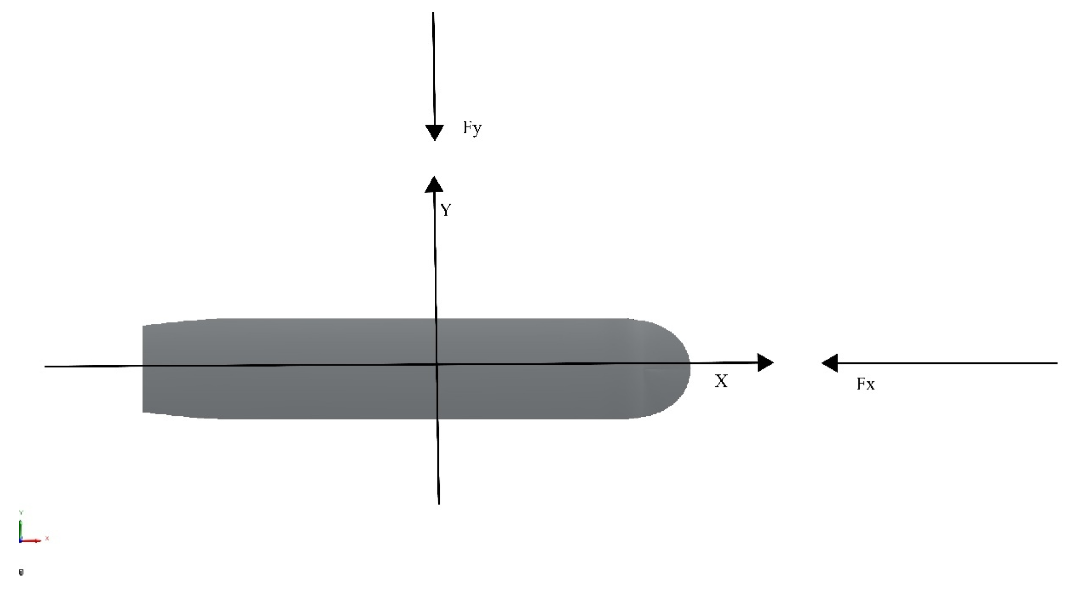
Figure 1: Wind resistance of a ship.
For the independence of the results, dimensionless treatment is required, so the wind load factor is calculated using the following formula:
Among them,
3 Calculation of Ship Wind Resistance
This chapter introduces the calculation process of numerical simulation software, covering the parameter setting and data processing before calculation. This paper calculates the ship wind load under the same wind speed conditions at different wind directions and compares it with the test data.
First, the hull is built using Rhino software. The 3D geometric model of the ship is imported into the STARCCM+ software for calculation. The geometric model is checked for geometric problems. After the geometric relationship is handled, the coordinate system is set. The hull general coordinate system is used. The X axis is along the length of the ship, the bow is positive; the Y axis is along the width of the ship, the port side is positive; the Z axis is vertically upward. After determining the calculation domain and coordinate system, a cube-shaped geometry is created around the 3D curved surface hull model that has been meshed and repaired according to the corresponding size. The hull is subtracted from the geometry through Boolean operations. The generated volume is a continuous and closed virtual towing test pool containing the ship. The entire area contains the hull, air and water. The mesh division of the calculation domain is mainly divided into three parts: the surface mesh of the hull surface, the boundary layer mesh where the hull contacts the water surface, and the volume mesh of the calculation domain. By creating an automatic mesh operation, the corresponding surface mesh, boundary layer mesh and volume mesh are generated by selecting surface reconstruction, automatic surface repair, cutting volume mesh unit generator, and prismatic layer mesh generator in sequence. Secondly, the mesh independence verification is conducted to ensure the accuracy of the results accurate. The comparison between the numerical simulation results obtained during the validation and wind tunnel experimental values also proved that this numerical simulation method is correct and feasible.
3.2 Numerical Simulation of Hull
3.2.1 Establishment of Hull Model
This paper takes a 67.6 m LNG-powered multipurpose ship as the research object. Its main ship parameters are shown in Table 1.
Table 1: Parameters of a 67.6 m LNG-powered multipurpose vessel.
| Main Scale | Unit | Quantity |
|---|---|---|
| Total length | M | 67.6 |
| Width | M | 12.66 |
| Depth | M | 4.40 |
| Design draft | M | 3.35/3.50 |
First, the ship type line drawing is imported into the Rhino software, with the transverse section drawing as the main part and the longitudinal section drawing as the auxiliary part. The surface entity between the two station lines is generated by the mesh surface command in the software and the appropriate mesh density is selected, and then the deck and stern plate are generated by the upper deck edge line, corner line, etc.; it is worth noting that the curvature of the stern propeller position varies greatly, and it needs to be generated separately with the help of the surface stitching function in the software to ensure the accuracy of the surface. Because the calculation is for the ship resistance, only the 67.6-m ship hull model needs to be established, as shown in Fig. 2. Thus, the three-dimensional model of the hull is obtained and then the model is imported into the simulation software for subsequent calculations. This paper mainly studies the wind resistance and wind resistance of ships, so only the model of the hull part above the design draft of the target ship needs to be considered.
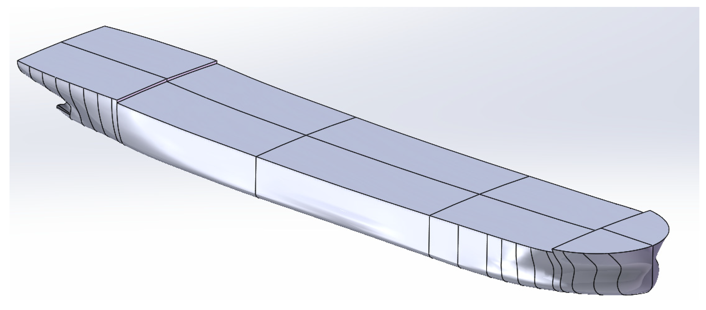
Figure 2: 3D model of a 67.6-m ship.
3.2.2 Determination of Computational Domain
In the process of numerical simulation of ship wind load calculation, the calculation domain must be reasonably determined first. That is, a flow field area including the hull is specified. It is very important to select a suitable domain for calculation. If it is determined to be too small, the flow field around the ship cannot be completely contained, which makes it difficult to capture the flow conditions well, and the calculated results will become unreliable; however, if the calculation domain is set too large, although the entire flow field can be included, it will cause a large amount of calculation, waste more computing resources, and the accumulated excessive numerical errors will make the results unreliable.
The layout of the computational domain selected in this paper determines the center of mass of the bottom surface of the ship as the origin, the bow direction as the X-axis, the vertically upward direction as the Z-axis, and the direction from the bow to the left as the Y-axis. Specifically: The computational domain size of this paper is: 1.5 times the hull length (1.5L) in front of the bow, 3 times the hull length (3L) behind the stern, 1.5 times the hull length (1.5L) on both sides of the ship’s width, and 1.5 times the hull length (1.5L) in the vertical direction to arrange the computational domain [19]. In this way, the computational domain can completely surround the flow field and meet the requirements of the blockage rate. The specific computational domain settings are shown in Fig. 3.
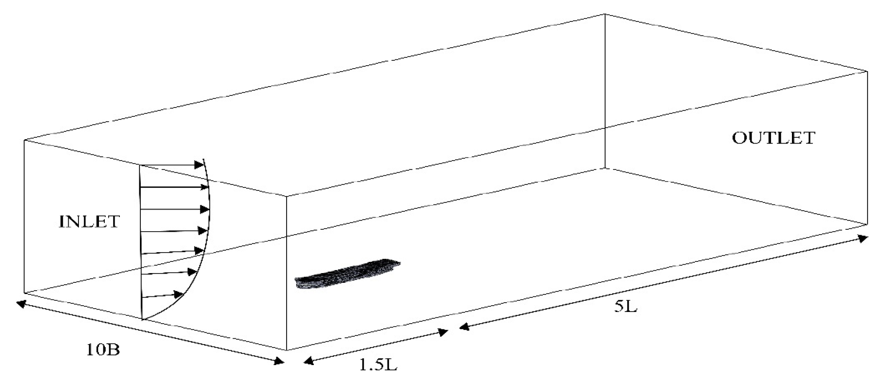
Figure 3: Computational domain diagram.
This paper uses an unstructured grid in the calculation process and uses Prism Layer The way Mesher generates boundary layer grids effectively ensures the accuracy of the flow on the ship surface and around the hull. When making the grid, the fluid area is divided into different areas by dividing the geometric model of the ship, and the grid is locally encrypted for the ship surface, wake vortex area, and boundary layer area. This can achieve a higher grid density in places where special needs are needed, thereby enhancing the accuracy of the flow in these places, especially the accuracy of important parts such as the tail and boundary layer, thereby preventing numerical errors caused by too sparse grids. As shown in Fig. 4.
For the boundary layer mesh case, we use Prism Layer the Meshto method captures the grid at the prism level to capture the boundary layer effect of turbulence. The Wall Y+ value is calculated and roughly set to 1 during the setting, and the turbulence model can operate normally inside and in the boundary layer. Set 8 to 12 prism layers, the height of the lowest layer is 0.02 m, and the growth rate is selected as 1.2, so that the grid gradually spreads to a farther distance. In addition, the height of the prism layer is set to 0.1 to 0.2 m to fully contain the boundary surface area. Grid quality is confirmed by quality inspection to confirm that there are no non-orthogonal units, torsion or degradation [20]. In this way, there will be no instability problems caused by grid quality problems or increased calculation errors; under the above reasonable grid division and optimization scheme, the simulation of the hull wind resistance was successfully completed. Detailed grids can determine the accurate capture of the boundary layer and wake area of the turbulence model, improve the local quality of the grid, and ensure the stability of the calculation process and correct results; grid optimization reduces resources such as grid calculation time and cost, ensuring a good calculation basis for subsequent turbulence simulation and wind resistance analysis. The final grid is shown in Fig. 4, Fig. 5 and Fig. 6.
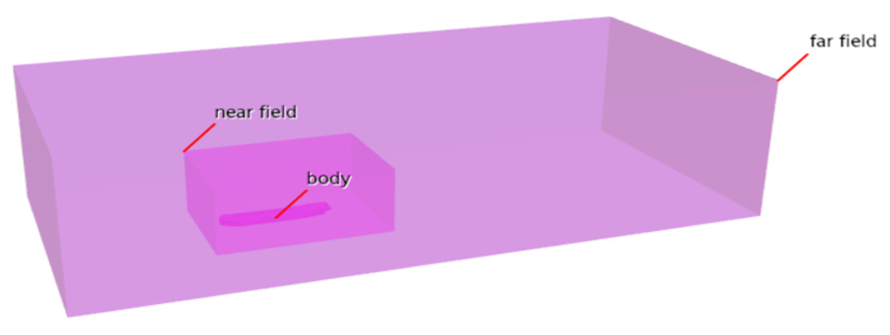
Figure 4: Range encryption settings.
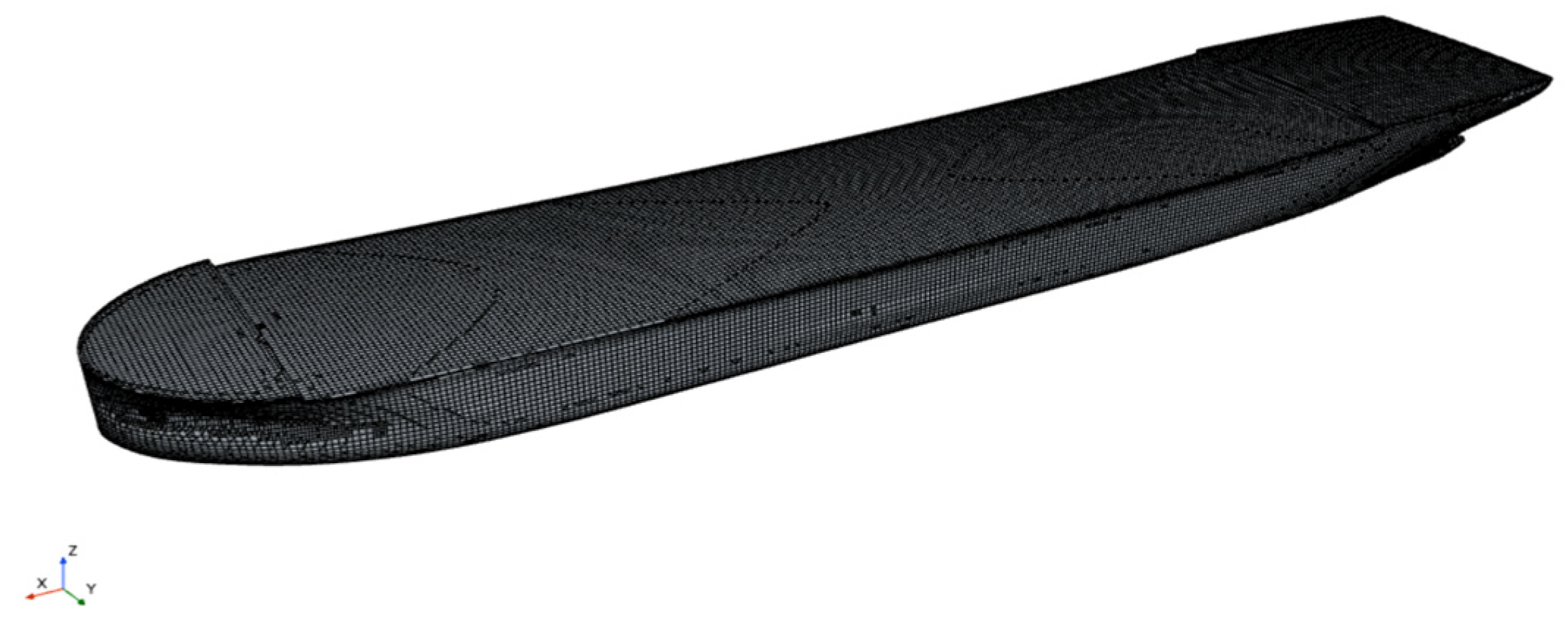
Figure 5: Hull surface grid diagram.
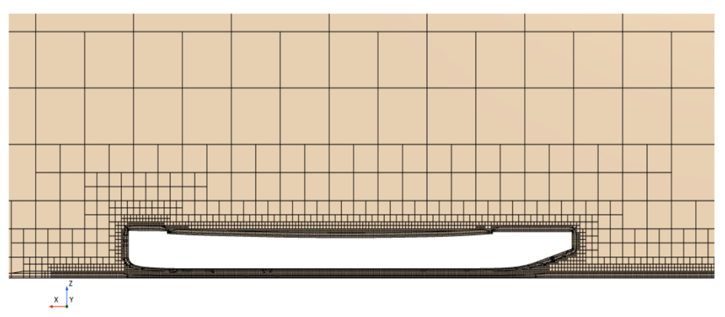
Figure 6: Mesh diagram around the hull.
In fluid simulation, boundary conditions are used to determine the motion characteristics of the fluid in a particular area and are an essential basis for solving the differential equation. To obtain a reliable and correct numerical simulation, it is necessary to correctly set appropriate boundary conditions for the fluid.
In this paper, the boundary conditions are set as shown in Fig. 7. In the figure, the hull surface and the top and bottom of the computational domain are set as wall boundaries. Since there is relative slip between the hull and the water surface, the bottom boundary is set as a slip wall [21]. The rest of the hull is considered to be fixed, so it is set as a non-slip wall and is impenetrable. For different boundaries of the pool, the velocity inlet and pressure outlet are set according to the requirements of the simulation conditions. For example, when the wind speed direction is at an angle of 30° to the X-axis, the pool inlet and the left side of the pool are set as the velocity inlet, and the pool outlet and the right side of the pool are set as the pressure outlet.
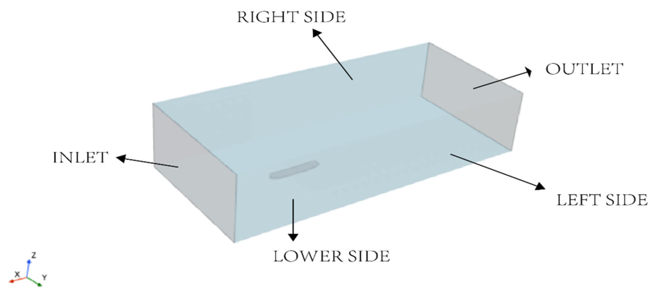
Figure 7: Boundary conditions diagram.
In this study, the k-ε model, which is widely used in engineering projects, was selected. Its advantage lies in that it does not require explicit wall function definitions in its equations, allowing it to accurately and stably handle complex boundary layer flows with pressure gradients, thus enabling more reliable simulation of wind pressure. The wind speed in the flow field is assumed to be uniform, which is a steady-state wind field. The density of air is assumed to be air for simplicity. The reference pressure is the atmospheric pressure at room temperature.
3.2.6 Grid Independence Verification
When applying wind resistance simulation to the hull surface, to obtain a more reliable numerical solution and ensure that the simulation accuracy is high enough, this simulation work has been tested for grid independence. The grid independence test is carried out by establishing a grid from sparse to dense for the model, and then determining whether the simulation results have a stable trend, that is, the size of the grid will not affect the calculation results. In the test process, three different levels of fineness of the grid settings are used, namely, the coarse grid, the medium-level grid and the fine grid. As shown in Table 2, different grid settings are used to simulate and calculate the wind resistance value and turbulent dissipation rate (TKE) of the hull surface under the same calculation area and boundary conditions. Then, by comparing the values of different grids, it is determined whether the simulation results have reached a stable state, and when the results are consistent, they can be regarded as grid-independent (Fig. 8). The final selected grid count is 1,240,166 (Table 3).
The test process of grid correlation is as follows: First, use the coarse grid to preliminarily solve the basic flow field: Then, further encrypt the grid based on the existing coarse grid and perform the grid test solution process with intermediate accuracy: The third step is to continue to encrypt the grid, especially in the boundary layer and wake area: Finally, compare the wind resistance numbers between different grids. If the difference in wind resistance numbers between the three grid settings is less than 2%, then it can be said that the solution has converged to this value. The test results shown in the figure show that the grid gradually becomes finer from coarse, and the results tend to be stable, with a difference in wind resistance numbers of less than 2%. From this, we can conclude that the current grid accuracy can meet the calculation requirements, and the impact on the calculation is negligible. This test method ensures that the simulation results of this article are stable and reliable, providing a reliable foundation for the subsequent analysis of turbulence and wind resistance.
Table 2: Mesh quantity modeling.
| Number of Model | 1 | 2 | 3 | 4 | 5 |
|---|---|---|---|---|---|
| Number of Meshes | 801,457 | 1,043,575 | 1,240,166 | 1,286,547 | 1,306,589 |
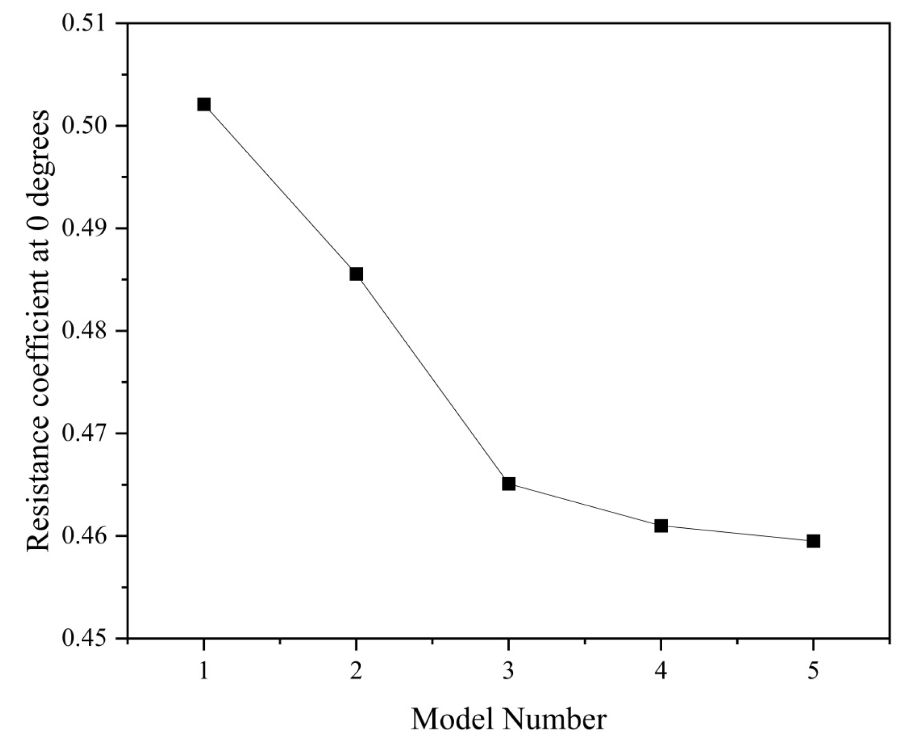
Figure 8: Grid independence verification.
Table 3: Mesh sensitivity analysis.
| Grid Type | Number of Meshes | Resistance Coefficient at 08 | Percentage Variation |
|---|---|---|---|
| Coarse | 801,457 | 0.505 | - |
| Medium | 1,043,575 | 0.485 | 3.96 |
| Fine | 1,240,166 | 0.465 | 4.12 |
| Finer | 1,286,547 | 0.462 | 0.64 |
| Ultra-fine | 1,306,589 | 0.460 | 0.43 |
3.3 Analysis of Calculation Results
3.3.1 Study on Wind Resistance Load
In this paper, wind resistance simulation calculations at multiple angles were performed to calculate the corresponding wind resistance coefficients at various angles when the wind speed was 2.0 m/s. According to the calculation requirements of wind resistance, wind directions of 0, 30, 60, 90, 120, 150, and 180 degrees were selected to perform numerical calculations on the ship. The data obtained from the simulation results are shown in Fig. 9 and Fig. 10.
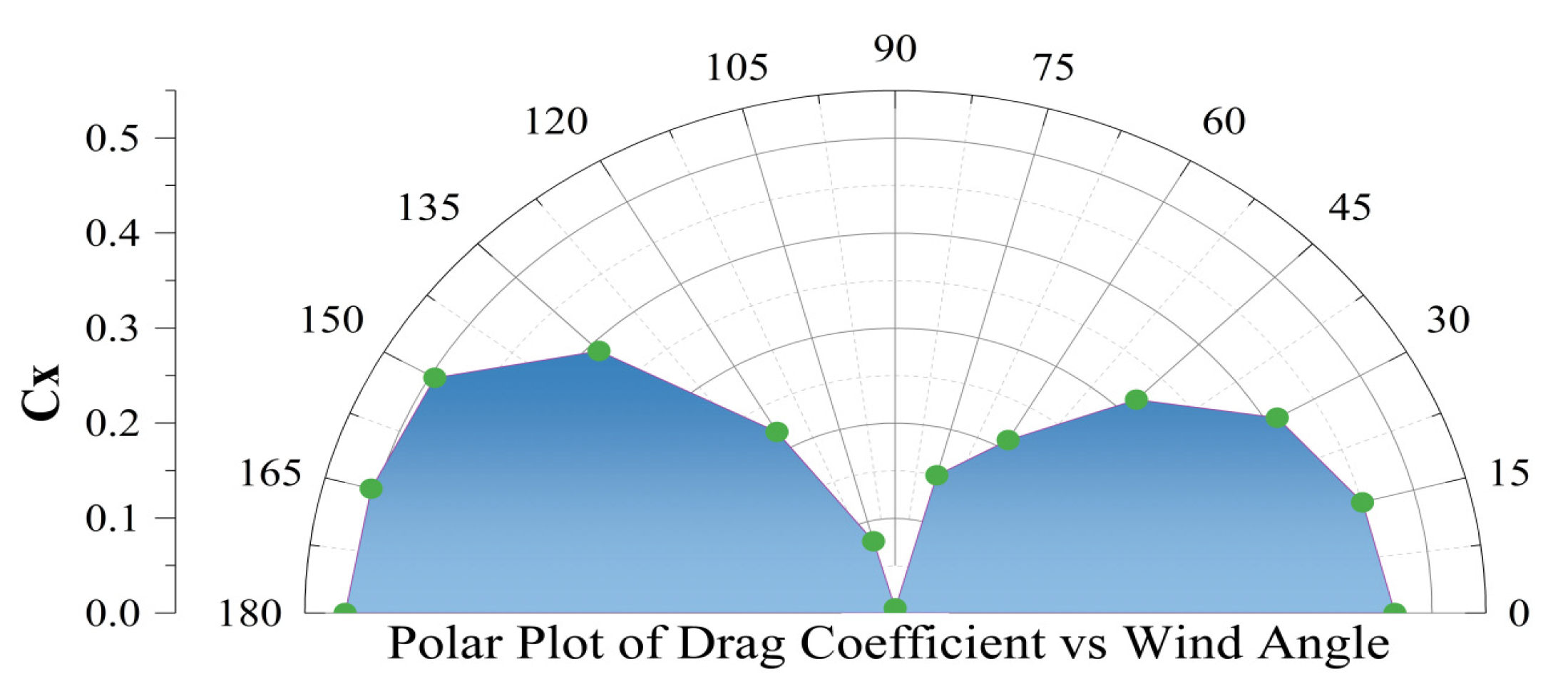
Figure 9: Drag coefficient CX diagram.
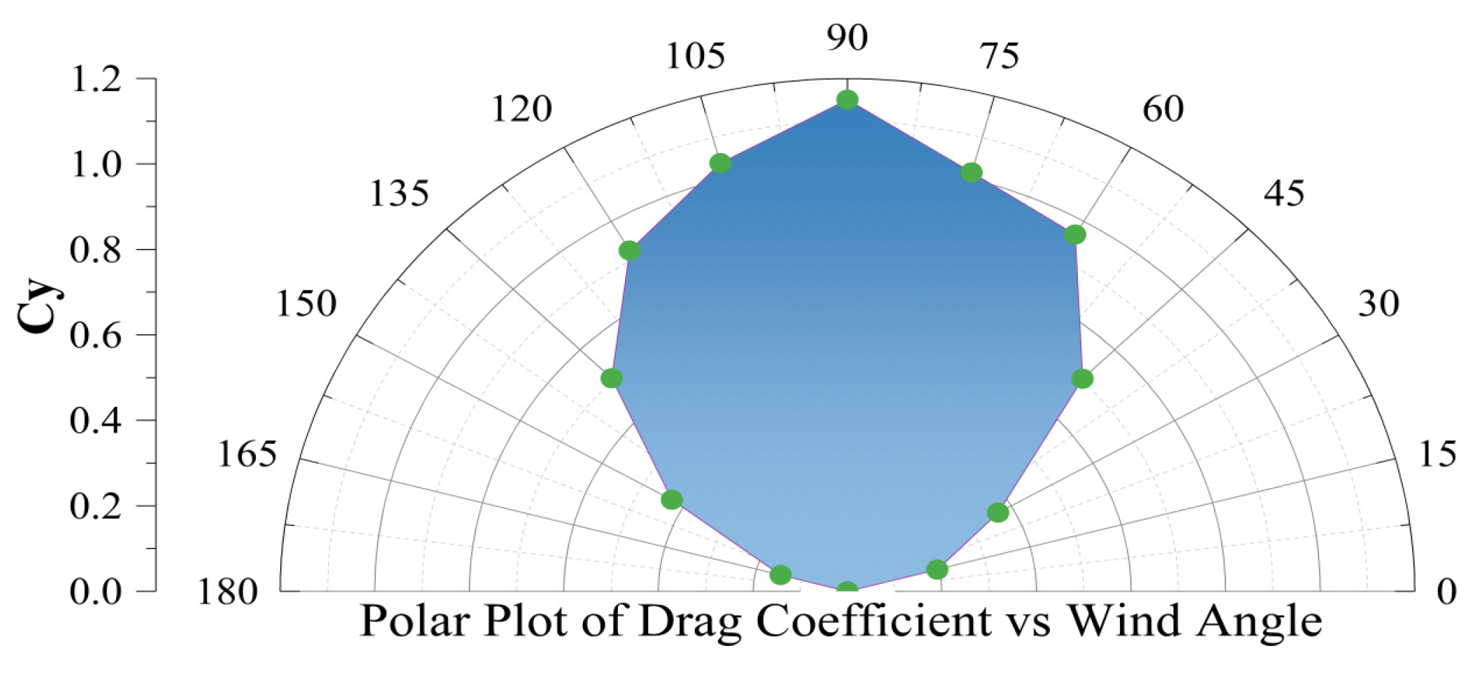
Figure 10: Drag coefficient CY setting.
The simulation results show that when the wind direction angle is 0°, the wind blows from the front to the bow, the windward area of the hull is the largest, and the strongest positive resistance is generated. CX reaches a local peak under this condition. As the wind direction angle increases, the wind direction gradually deviates from the bow, and CX shows a downward trend, drops to nearly 0 at 90°, indicating that the aerodynamic force mainly acts in the horizontal direction and the longitudinal component is extremely small. Continue to increase the wind direction angle, the wind direction turns to the stern, CX begins to rise, and reaches a higher value again at 180°. This trend reveals the inherent connection between the hull’s windward area and the aerodynamic force under different wind directions, that is, the change in the CX value is directly related to the exposed area of different parts of the hull.
At the same time, CY is close to 0 when the wind direction angle is 0° and 180°, which means that the lateral force is close to zero, but reaches the maximum value when the windward angle is 90°, which means that the wind has exerted the greatest lateral force on the hull. CY gradually increases when the windward angle changes from 0° to 90°, and then gradually decreases when the windward angle changes from 90° to 180°, showing a typical symmetrical nonlinear increase.
The simulation results obtained from the wind tunnel experiment are shown in Fig. 11 and Fig. 12.
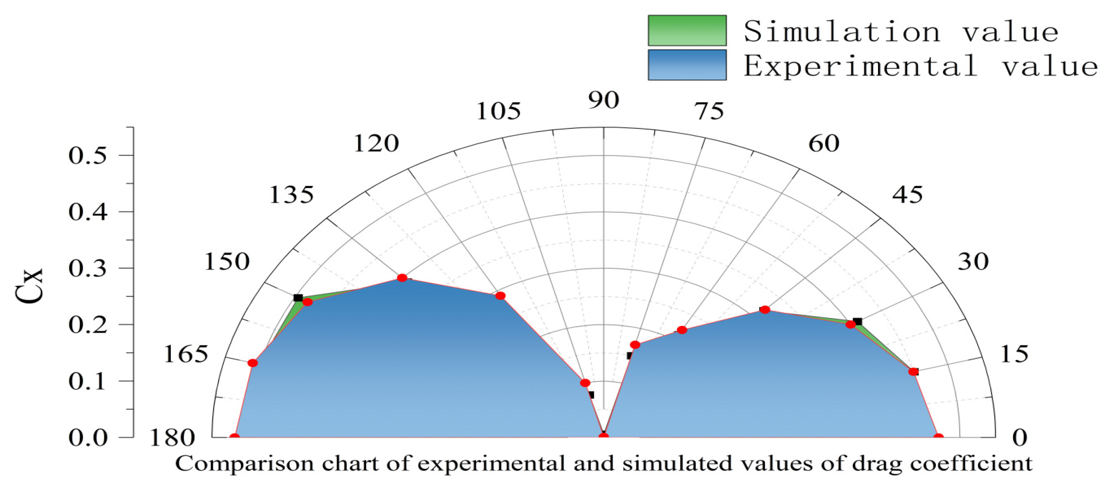
Figure 11: Drag coefficient CX diagram.
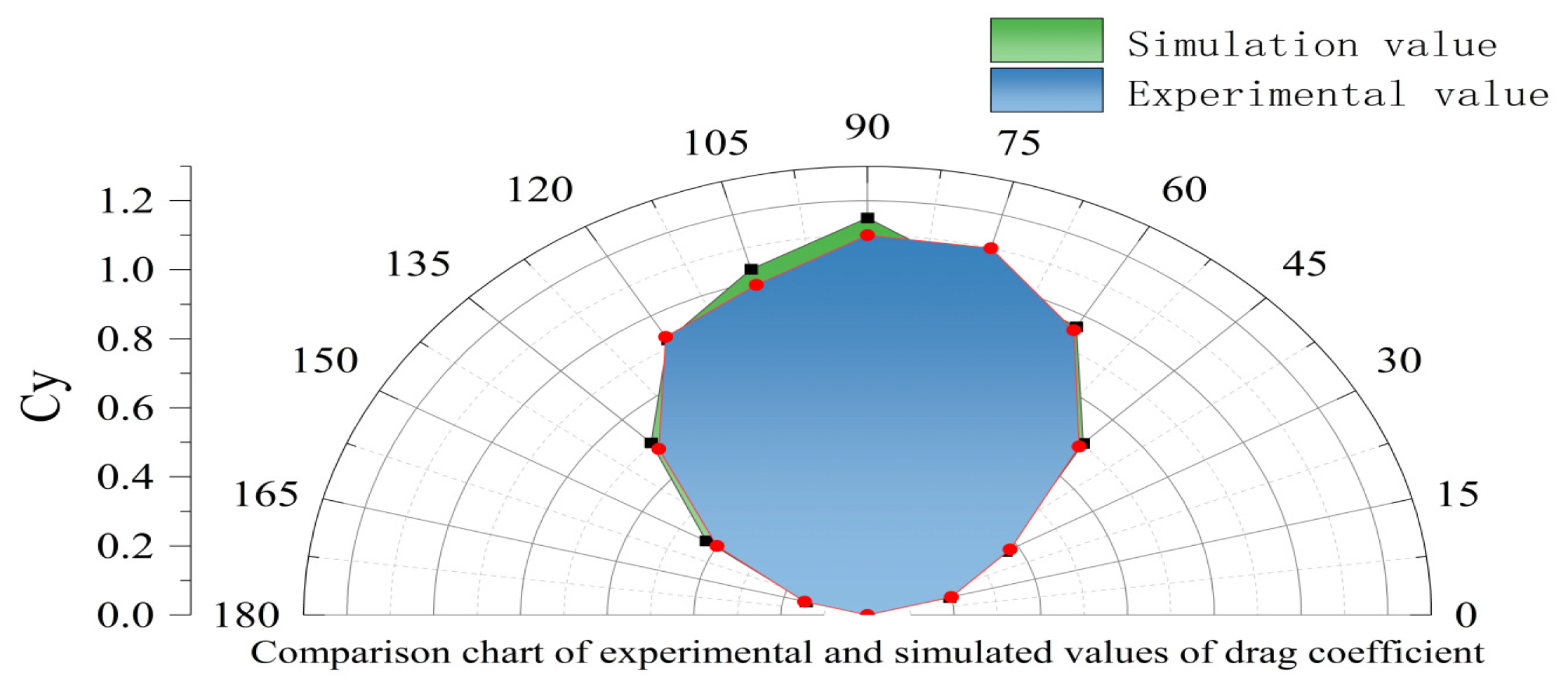
Figure 12: Drag coefficient CY diagram.
By comparing the pressure cloud diagrams on the ship’s surface, we can directly see the local and global changes that occur on the ship’s surface and as a whole as the windward angle changes, and explain the physical phenomenon behind the change in the wind lift coefficient, as shown in Fig. 13 and Fig. 14.
In the case of 0° incident wind direction, the wind blows directly at the bow, resulting in a relatively obvious high-pressure area at the windward side of the bow, especially at the intersection of the bow edge and the front arc. At the same time, low-pressure areas are formed on the side and stern of the ship when air flows through, and a relatively strong tail vortex structure and negative pressure area are formed at the stern. This high-low pressure area distribution causes a significant one-to-one pressure unevenness, which leads to the main cause of resistance (CX is large) and is the location of the largest resistance generation area. Subsequently, as the wind direction angle increases from small to large until 90°, the flow mainly affects the side of the ship and other directions. A high positive pressure area forms on one side of the hull surface, while a lower negative pressure area is formed on the other side due to the combined influence of airflow separation, backflow and other factors. Under this condition, a large pressure asymmetry distribution pattern is formed, which leads to the maximum value of CY; the pressure balance point is obviously offset from the middle position line, and a certain wind-pushed horizontal thrust property is revealed. Next, as the wind direction angle changes to 180°, the wind blows towards the stern. At this time, a high positive pressure distribution is generated in the stern area, and a large negative pressure area appears in the bow area under the action of the airflow suction force. This form is basically the same as the previous 0° angle, except that it is completely reversed. Similarly, it will form a relatively high positive aerodynamic force in the X direction. Since the stern is often blunt or flat, it has more separated airflow and a stronger tail vortex, which will also cause local pressure instability.
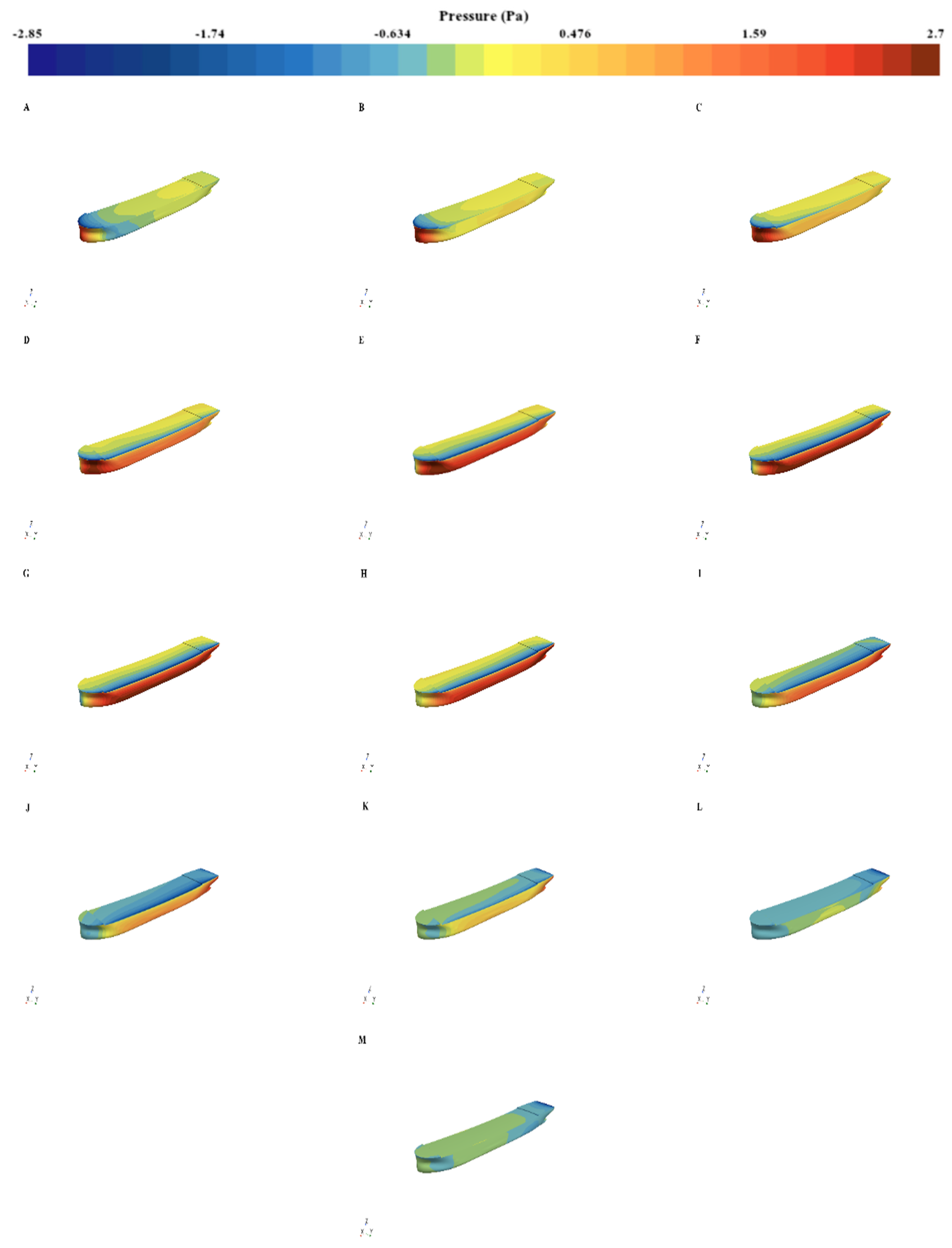
Figure 13: The numerical wind pressure distribution of a 67.6-m ship under different wind directions in the range of θ = 0° to 180° (every 15°), where (A–M) correspond to each wind direction.
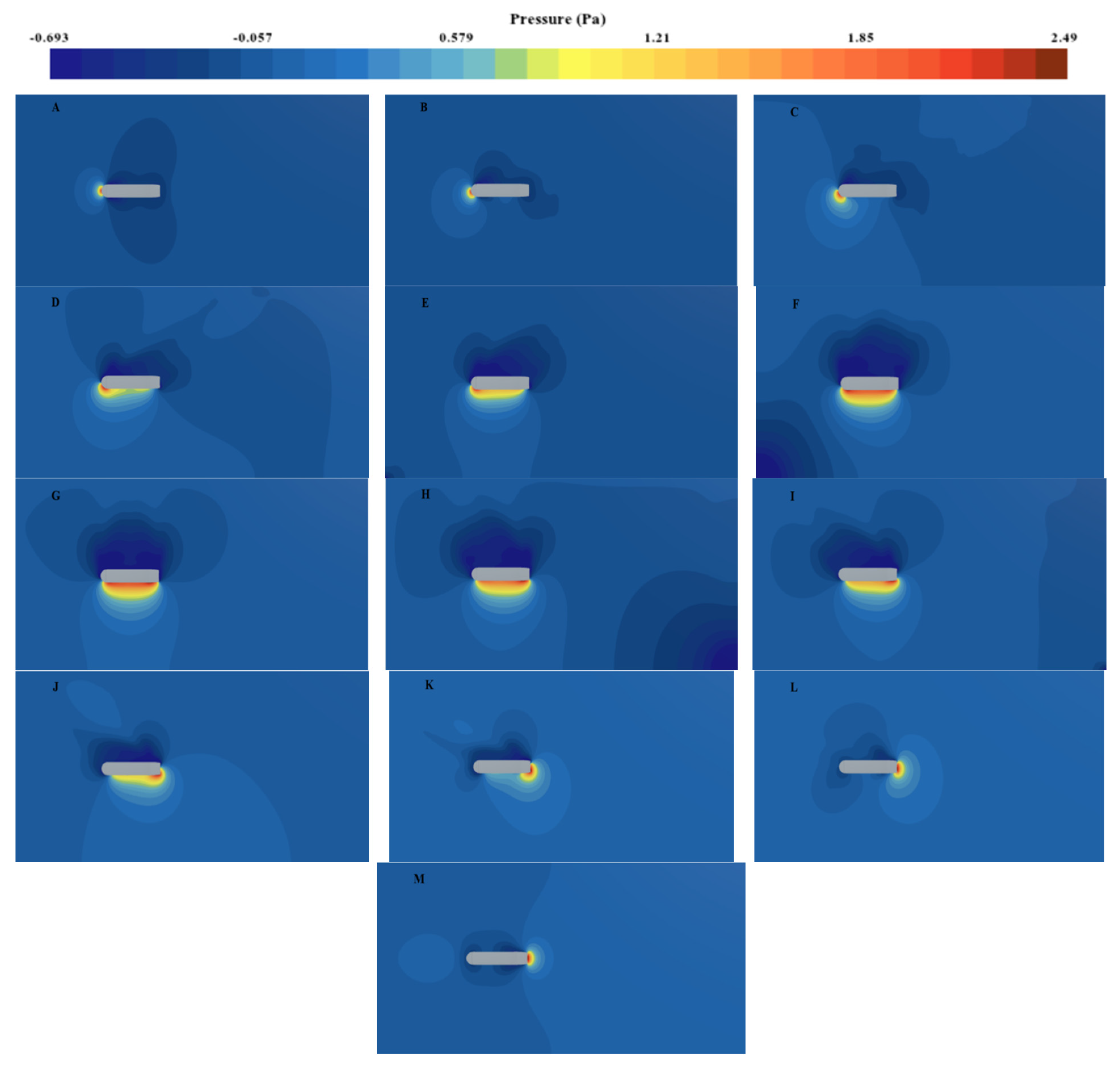
Figure 14: The numerical wind pressure distribution around a 67.6 m ship under different wind directions in the range of θ = 0° to 180° (every 15°), where (A–M) correspond to each wind direction.
Under different crosswind angles, the velocity field around the ship presents different distribution forms, which directly affect the aerodynamic characteristics of the hull. As shown in Fig. 15. Under the crosswind angle of 0°, the airflow hits the bow head-on, generating symmetrical flow, forming an obvious low-speed area and local separation in front of the bow, while a typical tail vortex flow is generated in the rear stern area. As the crosswind angle increases to 45° and 75°, the airflow field is asymmetrically distributed, the flow field on one side of the ship accelerates, and there is a shear layer and a recirculation area on the leeward side, and the airflow becomes complicated. In the case of a 90° crosswind, the airflow blows vertically into the hull, causing a side impact on the ship. The velocity on the windward side slows down significantly, but there is a large amount of recirculation on the leeward side of the ship, forming an asymmetric wake structure behind the ship. Under the action of a 180° crosswind angle, the airflow enters the flow field along the stern direction, and a large stagnation and negative velocity area appear at the stern of the hull, and the suction of the bow causes local accelerated flow. In summary, it can be seen that under the action of various side wind angles, the influence of the flow field on the flow velocity on the hull surface varies greatly, and the resulting flow field structure at the rear of the hull is also different. The velocity distribution law is basically consistent with the change trend of the drag coefficient, which can provide a strong data basis for subsequent optimization designs of related aerodynamic shapes.
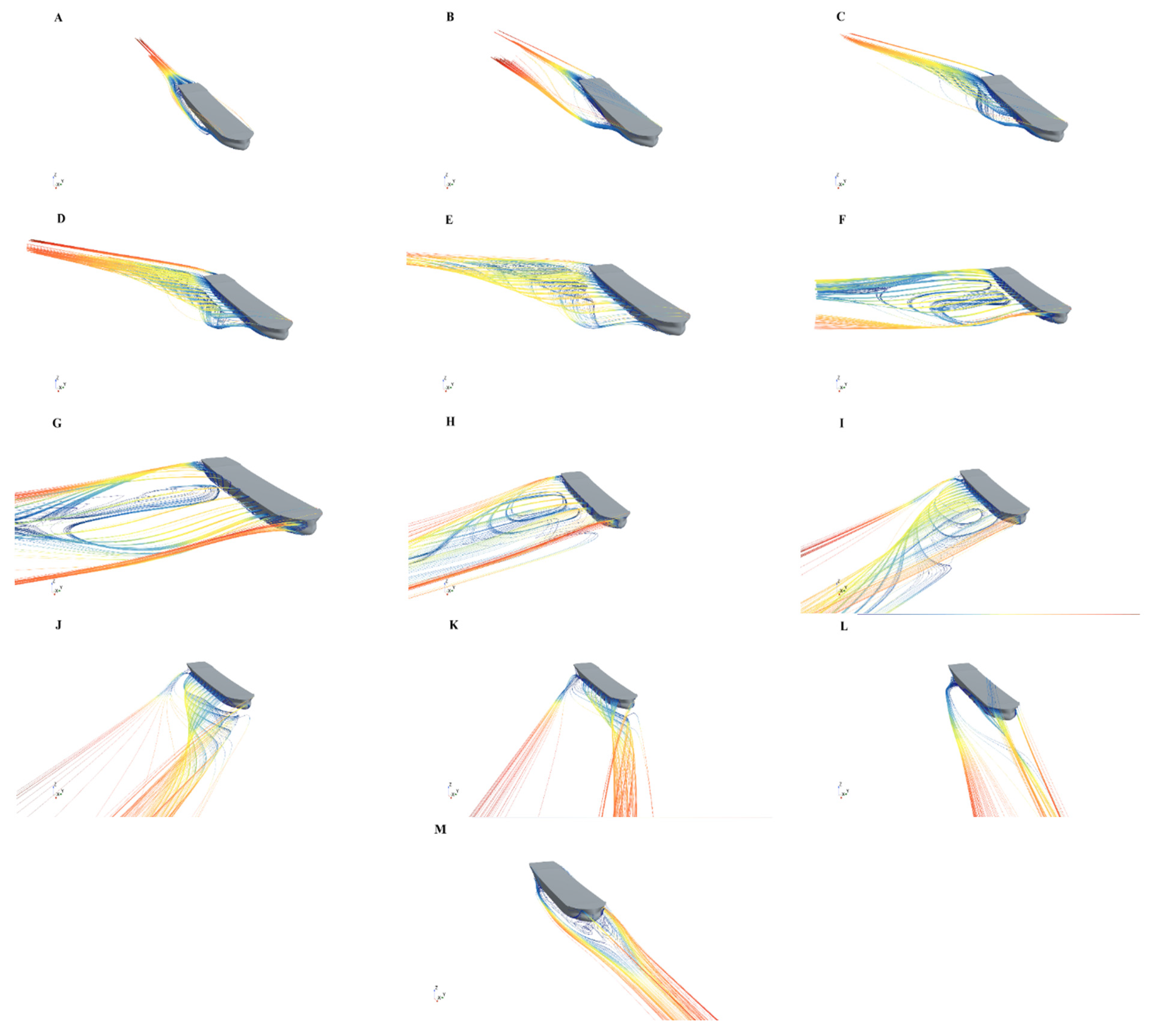
Figure 15: Numerical streamline distribution of a 67.6 m ship under different wind directions (θ = 0°–180°, every 15°), where (A–M) correspond to each wind direction.
With the continuous advancement of energy conservation, emission reduction and green shipping concepts, optimizing ship aerodynamic performance has long been an indispensable key factor. In a sailing environment with significant wind force, reducing wind resistance, improving propulsion efficiency and reducing energy consumption are of great significance to improving the comprehensive performance of ships. Under this goal, this paper studies the wind resistance characteristics of ships under different wind angles, combines CFD numerical simulation methods, systematically analyzes the impact of wind direction changes on the aerodynamic forces on the hull, and puts forward targeted structural optimization suggestions based on the results.
In this study, a 3D geometric model and a numerical simulation model were established using relevant 3D and simulation software, respectively. The changes in the drag coefficient were compared under 13 typical working conditions, with wind direction angles ranging from 0° to 180° and at 15° intervals. In order to more intuitively reflect the influence of the wind direction on the aerodynamic force of the hull, this paper decomposes the wind resistance coefficient into two components: CX in the downwind direction and CY in the perpendicular wind direction. Through simulation, it is found that when the wind direction angle is 0°, the wind acts on the bow position, at which time the frontal resistance of the hull is the largest, CX reaches the peak value, and CY is almost zero; when the wind direction angle increases to 90°, the wind blows directly to the side of the hull, causing the lateral aerodynamic force to increase significantly, CY reaches the maximum at this time, and CX is close to zero or even has a slight change trend; when the wind direction angle continues to increase to 180°, the wind mainly acts on the stern, forming a certain reverse resistance, causing CX to increase again, and CY gradually returns to a state close to zero.
Further analysis found that the change in wind direction not only changes the magnitude of wind resistance but also affects the distribution characteristics of its acting direction. At some wind direction angles (such as 60°, 75°, 105°, 120°, etc.), the wind exerts a compound effect on the hull, resulting in both CX and CY having large values. Especially in the area where the crosswind angle is close to 90°, the wind easily forms a high-pressure area on the windward side of the hull during the flow process, and at the same time generates a low-pressure vortex area on the leeward side, causing unstable forces on the hull and additional energy consumption.
After clarifying the trend of wind resistance changes, this article discusses how to reduce wind resistance by optimizing the hull structure design, especially in high wind pressure areas. By analyzing the wind pressure distribution characteristics of the bow, stern and other parts, optimization ideas can be provided for ship designers. For example, adding a windshield structure to the bow or changing the vertical surface of the hull to a streamlined inclined surface design can effectively reduce the direct impact of wind on the hull. Provide a new solution for future ship designers to reduce wind resistance by improving the hull shape. Especially under extreme working conditions such as 0° and 90°, the optimization of the ship’s aerodynamic performance will significantly contribute to improving ship efficiency, reducing energy consumption and emissions.
In summary, this paper systematically simulates and analyzes the variation of wind resistance of ships under typical wind angles, and proposes a series of structural optimization ideas, which not only provide theoretical support and engineering reference for future improvements in ship aerodynamic performance, but also verify the feasibility of wind resistance prediction and design adjustment based on CFD methods. Future work can introduce more actual operating conditions and wind field uncertainty factors on this basis to further improve the adaptability and energy-saving performance of ships in complex environments.
Acknowledgement:
Funding Statement: This research was funded by Shandong Province Key R&D Program (Innovation Capacity Improvement Project for Science and Technology Small and Medium-Sized Enterprises) Project No.: 2025TSGCCZZB0679 and Project ZR2024QE394 supported by Shandong Provincial Natural Science Foundation.
Author Contributions: Conceptualization, Jichao Li and Guang Chen; methodology, Fanpeng Kong; software, Yi Guo; validation, Guang Chen; formal analysis, Zhiming Zhang; investigation, Lingchong Hu; resources, Shiwang Dang; data curation, Xue Pei; writing—original draft preparation, Shiwang Dang; writing—review and editing, Jichao Li; visualization, Lingchong Hu; supervision, Zhiming Zhang; project administration, Guang Chen and Jichao Li; funding acquisition, Yi Guo. All authors reviewed the results and approved the final version of manuscript.
Availability of Data and Materials: The data that support the findings of this study are available from the corresponding author upon reasonable request.
Ethics Approval: Not applicable.
Conflicts of Interest: The authors declare no conflicts of interest to report regarding the present study.
References
1. Aouimer Y , Boutchicha D , Hamoudi B . Numerical and experimental study of fluid-structure interaction of a marine propeller. Int Rev Mech Eng. 2020; 14( 5): 282– 9. doi:10.15866/ireme.v14i5.17582. [Google Scholar] [CrossRef]
2. Majidian H , Azarsina F . Aerodynamic simulation of a containership to evaluate cargo configuration effect on frontal wind loads. China Ocean Eng. 2018; 32( 2): 196– 205. doi:10.1007/s13344-018-0021-1. [Google Scholar] [CrossRef]
3. Zhang R , Huang L , Ma R , Peng G , Ruan Z , Wang C , et al. Numerical investigation on the effects of heel on the aerodynamic performance of wing sails. Ocean Eng. 2024; 305: 117897. doi:10.1016/j.oceaneng.2024.117897. [Google Scholar] [CrossRef]
4. Hordiienko OL , Pechenyuk AV . Development of propulsion solutions for river-sea ships of the northern black sea. Proc Inst Mech Eng. 2024; 238( 2): 325– 35. doi:10.1177/14750902231203443. [Google Scholar] [CrossRef]
5. Grlj CG , Degiuli N , Tuković Ž , Farkas A , Martić I . The effect of loading conditions and ship speed on the wind and air resistance of a containership. Ocean Eng. 2023; 273: 113991. doi:10.1016/j.oceaneng.2023.113991. [Google Scholar] [CrossRef]
6. Ricci A , Janssen WD , van Wijhe HJ , Blocken B . CFD simulation of wind forces on ships in ports: case study for the rotterdam cruise terminal. J Wind Eng Ring Ind Aerodyn. 2020; 205: 104315. doi:10.1016/j.jweia.2020.104315. [Google Scholar] [CrossRef]
7. Wang Y , Chen X . Evaluation of wind loads on high-rise buildings at various angles of attack by wall-modeled large-eddy simulation. J Wind Eng Ind Aerodyn. 2022; 229: 105160. doi:10.1016/j.jweia.2022.105160. [Google Scholar] [CrossRef]
8. Saydam ZA , Taylan M . Evaluation of wind loads on ships by CFD analysis. Ocean Eng. 2018; 158: 54– 63. doi:10.1016/j.oceaneng.2018.03.071. [Google Scholar] [CrossRef]
9. Forrest JS , Owen I . An investigation of ship air wakes using detached-eddy simulation. Comput Fluids. 2009; 39( 4): 656– 73. doi:10.1016/j.compfluid.2009.11.002. [Google Scholar] [CrossRef]
10. Ticu I , Popa I , Ristea M . The rigid bi-functional sail, new concept concerning the reduction of the drag of ships. IOP Conf Ser Mater Sci Eng. 2015; 95( 1): 012070. doi:10.1088/1757-899X/95/1/012070. [Google Scholar] [CrossRef]
11. Kitamura F , Ueno M , Fujiwara T , Sogihara N . Estimation of above water structural parameters and wind loads on ships. Ships Offshore Struct. 2017; 12( 8): 1100– 8. doi:10.1080/17445302.2017.1316556. [Google Scholar] [CrossRef]
12. Janssen WD , Blocken B , van Wijhe H . CFD simulations of wind loads on a container ship: validation and impact of geometrical simplifications. J Wind Eng Ind Aerodyn. 2017; 166: 106– 16. doi:10.1016/j.jweia.2017.03.015. [Google Scholar] [CrossRef]
13. Wang W , Wu T , Zhao D , Guo C , Luo W , Pang Y . Experimental-numerical analysis of added resistance to container ships under presence of wind-wave loads. PLoS One. 2019; 14( 8): e0221453. doi:10.1371/journal.pone.0221453. [Google Scholar] [CrossRef]
14. Seo S , Park S , Koo BY . Effect of wave periods on added resistance and motions of a ship in head sea simulations. Ocean Eng. 2017; 137: 309– 27. doi:10.1016/j.oceaneng.2017.04.009. [Google Scholar] [CrossRef]
15. Kambe T . New perspectives on mass conservation law and waves in fluid mechanics. Fluid Dyn Res. 2020; 52( 3): 031401. doi:10.1088/1873-7005/ab93e0. [Google Scholar] [CrossRef]
16. Song KW , Xu P , Ge SW , Yang HY , Ma JC . Study on the influence of baffles on the hydrodynamic performance of ships in oblique navigation based on CFD. Ships. 2025; 36( 2): 52– 9. (In Chinese). doi:10.19423/j.cnki.31-1561/u.2024.024. [Google Scholar] [CrossRef]
17. Duraisamy K , Iaccarino G , Xiao H . Turbulence modeling in the age of data. Annu Rev Fluid Mech. 2019; 51( 1): 357– 77. doi:10.1146/annurev-fluid-010518-040547. [Google Scholar] [CrossRef]
18. Abu-Hamdeh NH , Almitani KH , Gari AA , Alimoradi A , Sun C . FVM method based on k − ε model to simulate the turbulent convection of nanofluid through the heat exchanger porous media. J Therm Anal Calorim. 2021; 144( 6): 2689– 98. doi:10.1007/s10973-020-10538-9. [Google Scholar] [CrossRef]
19. Li H , Chen X . Numerical method and analysis for fluid-structure model on unbounded domains. Appl Numer Math. 2025; 217: 255– 77. doi:10.1016/j.apnum.2025.06.009. [Google Scholar] [CrossRef]
20. Kodama Y , Hirota M , Kobayashi H . Generation of structured grids using shrink and recover algorithm. J Mar Sci Technol. 2025; 30( 2): 1– 15. doi:10.1007/s00773-025-01061-3. [Google Scholar] [CrossRef]
21. Zhang T , Zhou B , Liu H , Wu Z , Han X , Gho WM . A study on hydrodynamic analysis of ship with forward-speed based on a time domain boundary element method. Eng Anal Bound Elem. 2021; 128: 216– 26. doi:10.1016/j.enganabound.2021.04.007. [Google Scholar] [CrossRef]
Cite This Article
 Copyright © 2025 The Author(s). Published by Tech Science Press.
This work is licensed under a Creative Commons Attribution 4.0 International License , which permits unrestricted use, distribution, and reproduction in any medium, provided the original work is properly cited.
 Downloads
 Citation Tools