Deep Learning-Based Prediction of Seepage Flow in Soil-Like Porous Media

1 Introduction

Accurately evaluating fluid flow in saturated porous materials is critically important [1,2]. Soil, as a typical porous medium, is widely distributed in nature. The investigation of seepage behavior in soil is highly significant and has broad applications in areas such as water resources management and oil exploration [3]. However, the pore structure of soil exhibits complex heterogeneous and anisotropic characteristics [4], which lead to highly complicated fluid transport processes that are difficult to accurately capture with theoretical models [5]. Although experimental methods for seepage analysis can provide accurate predictions, they often involve drawbacks such as long durations, high costs, and limitations in capturing spatial heterogeneity [6,7].

With the gradual advancement of computer technology, numerical simulation has achieved the simulation of fluid flow in porous media at a very low cost, thereby revealing flow characteristics inside the porous media [8,9]. In numerical studies of flow in porous media, the acquisition of pore structure is primarily accomplished through CT scanning or stochastic generation methods [10,11]. CT scanning can capture the morphology of real porous media, from which flow behavior under actual pore structures can be derived via numerical simulation [12,13]. However, flow characteristics in porous media are strongly influenced by pore structure and morphology [14,15]. To derive more generalizable conclusions, it is necessary to investigate a wide range of porous media. Thus, the approach of using randomly generated porous structures to analogically represent various porous materials allows rapid and cost-effective generation of numerous pore-scale models. Flow simulations can then be performed to obtain broadly applicable findings [16,17]. There are various methods for random generation of porous media, including the Quartet Structure Generation Set [18,19], the geology process-based method [20], Markov Chain Monte Carlo [21] and Simulated Annealing [22]. Among them, the QSGS method enables rapid generation of porous media with consistent statistical characteristics through macroscopic control parameters [23]. Studies have demonstrated that QSGS is significantly faster than the SA algorithm for generating large-volume 3D porous structures, offering a feasible pathway for producing extensive datasets to enhance research sampling [24,25]. Many researchers have employed the QSGS method to characterize various porous materials, such as clays [26,27] or rocks [28,29]. Numerical methods for simulating fluid flow in porous media can be categorized into three groups based on scale: macroscopic scale, mesoscopic scale and microscopic scale [30,31]. Among them, the lattice Boltzmann method (LBM) is computationally efficient due to its ability to handle complex geometries and avoid the high computational overhead of mesh-based methods like the finite volume or finite element methods. When combined with graphics processing unit (GPU) acceleration, which leverages the local computation features of LBM, the speed advantage becomes even more pronounced [32]. Studies have reported that GPU-parallelized LBM simulation has increased the overall computing speed by 7 to 15 times [33,34]. Therefore, the LBM calculation method has been successfully applied in industrial simulations related to coal mines, natural gas extraction, and ceramics [35,36].

With the rapid development of artificial intelligence, machine learning (ML) has achieved significant progress in addressing various scientific and engineering problems, including flow analysis [37,38] and mechanical property prediction [39,40,41]. In particular, seepage prediction methods that integrate pore-scale numerical simulation with machine learning have emerged as a research hotspot, as they enable rapid analysis and synthesis of diverse porous structures [42,43]. Convolutional neural network (CNN), which utilizes convolutional and pooling layers to automatically extract key features from images, has shown great potential for image-based parameter prediction [44,45]. By combining large datasets of porous media samples generated by QSGS with CNN-based image recognition, it is possible to directly simulate and train models for fluid flow through these structures, thereby predicting the seepage characteristics of real porous materials [46]. For instance, Kamrava et al. [47] proposed a novel hybrid neural network architecture that combines the strengths of deep learning (DL) and traditional artificial neural networks (ANN). Trained on hundreds of randomly generated porous media samples produced by a reconstruction algorithm, their model successfully established an accurate correlation between pore morphology and permeability. Liu et al. [48] constructed a CNN capable of predicting permeability directly from structural images, and demonstrated its successful application to Berea and Bentheimer sandstones. Sudakov et al. [49] systematically assessed the applicability of machine learning technology for rock permeability prediction using a 3D image dataset of Berea sandstone and corresponding pore-network simulated permeability values. Their work innovatively integrated Minkowski functionals with deep learning-derived image descriptors, ultimately developing a highly accurate 3D CNN prediction model.

As evidenced by the literature, it is feasible to accurately predict fluid flow through porous media with realistic morphologies by training a CNN model using extensive soil-like porous structures generated via the QSGS method, along with flow simulation results efficiently computed by the LBM model accelerated with GPU parallel computing as the training dataset. However, the image-based CNN prediction method has certain problems. It has a high demand for the sample size of the training dataset, which poses extremely high requirements for computing resources. In the research of Sudakov et al. [49], 9261 samples were used for model training; while Zhang et al. [50] employed 25,000 samples in their dataset. The requirement for such voluminous data not only increases the computational cost of machine learning-based predictions but also prolongs the model preparation time, thereby diminishing the practicality and convenience of using these methods for seepage prediction in porous media.

To improve the efficiency of the entire process training, this study proposes a novel prediction method. The method begins by converting QSGS-generated porous structures into two primary control parameters based on a statistical averaging principle. These two parameters, together with a key seepage property—applied pressure difference, are used as input to establish a fully numerically operated deep learning model for predicting seepage flow. Compared to image-based CNN prediction methods, the proposed framework offers two main advantages: 1. This method firstly conducts specific feature extraction on porous medium images through the statistical idea of volume averaging, which is more targeted than the feature extraction of CNN. This helps to establish more accurate machine learning connection relationships, improve prediction accuracy and decrease the amount of data required for training. 2. The model utilizes a learning architecture based on numerical transformation, avoiding the loss of fine-grained spatial information inherent in the pooling operations of typical CNNs. To validate the feasibility of the proposed method in this study, this research first generated a set of porous media using QSGS, and performed flow simulations via an established LBM approach. The obtained parameters were used as the input parameters to train a deep learning model.

The following structure of this article includes the introduction of the established model, the macroscopic control equations of the flow and seepage of porous media and their control equations at the mesoscopic scale, the introduction of the process of generating porous media by QSGS, and the all-digital transfer MLP machine learning model; Immediately following is the verification of the established mesoscopic-scale seepage model. In this study, Poiseuille flow with analytical solutions was adopted for verification. Finally, the flow behavior in porous media simulated by the model is analyzed, the influence of QSGS parameters on flow characteristics and pore size is quantified, and the prediction accuracy of the model is evaluated.

2 Methods

2.1 Porous Media Generation

During the generation process, each point in the computational domain is initially assigned a random number. This value is compared with the preset core growth probability pcore: If the random number is greater than the pcore, this point is designated as a solid phase; otherwise, it is marked as a liquid phase point. Subsequently, one of the solid-phase points is randomly chosen as the basic point. The larger the pcore is, the more solid phase blocks are generated, the more pores the formed porous medium has, and the smaller the average pore size is. For adjacent points of this basic point, the random number and the growth probability pD of this direction are determined: if the random number is greater than pD, the adjacent points will change to the solid phase. If it is less than pD, the liquid phase is maintained. The larger the pD value is, the more easily the surrounding points will turn into a solid state. This also leads to the formation of larger and more compact solid blocks, and results in a larger average pore diameter of the porous medium. After each growth cycle, the total number of solid-phase points is calculated and compared against the target solid fraction. The process terminates when the desired proportion is reached. Otherwise, a new nucleation seed is randomly chosen, and the growth steps repeat until the target is met. By carefully controlling the growth target ratio, core formation probability pcore and growth probability pD in each direction of the two composite materials, a wide range of composite microstructures can be effectively represented. Fig. 1b depicts the example of the calculation domain for a porous medium structure generated by this method, with pcore being 0.05 and porosity being 0.5. During the LBM calculation, this porous media is divided into Lx ∗ Ly lattices for collision and streaming calculations, with Ly = Lx + 20. To ensure that the flow within the porous medium achieves a fully stable flow, 10 compartments of flow buffer zones are reserved at the inlet and outlet, respectively.

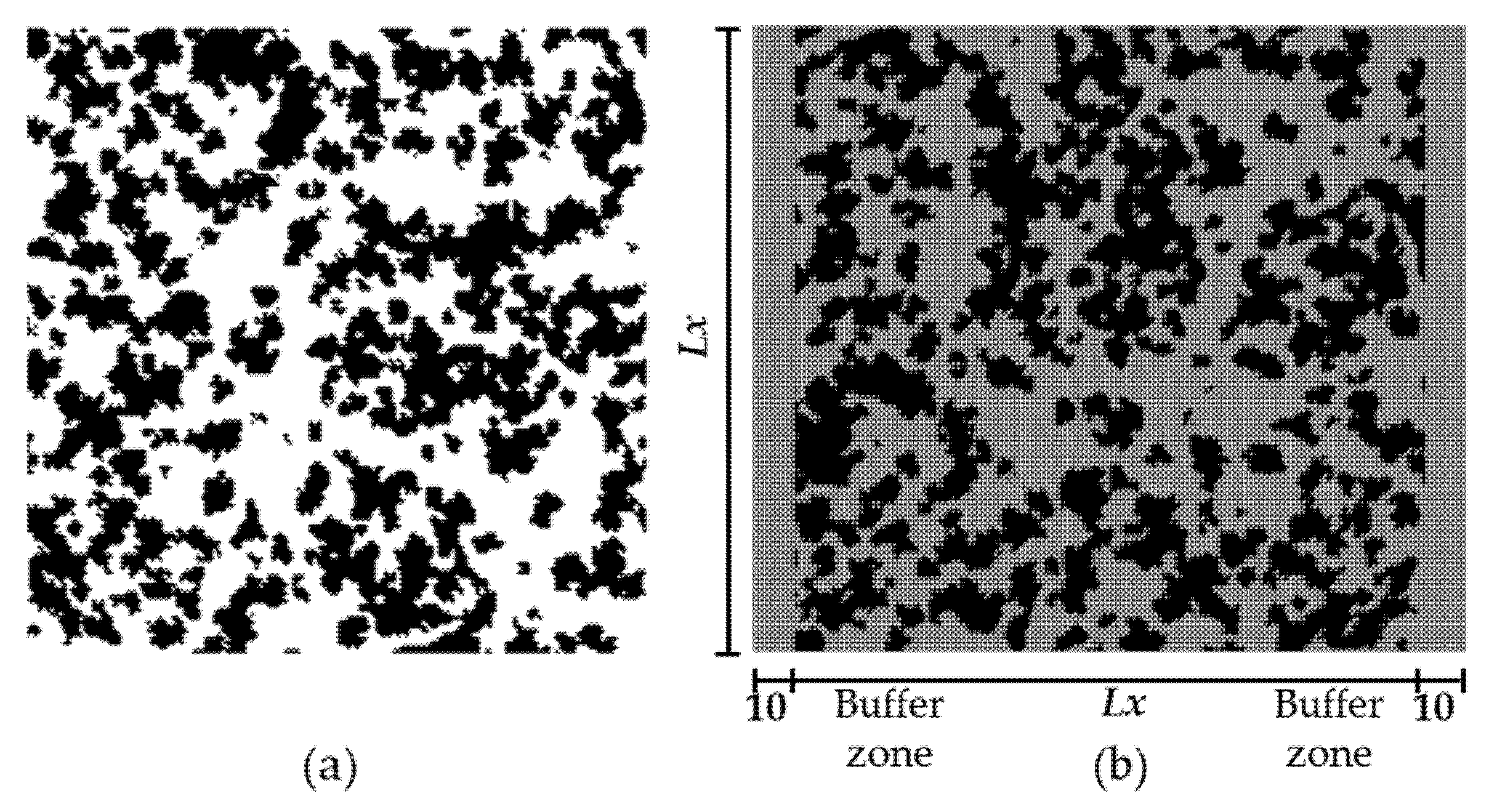
Figure 1: Description of the generated porous media (a) and corresponding calculation domain (b).

2.2 Flow Simulation

2.2.1 The Macroscopic Governing Equation

The movement of water through soil is fundamentally governed by physical conservation laws. The conservation of mass dictates the dynamic distribution of water, ensuring the balance among water inflow, outflow and storage within the soil. During flow, water is driven by pressure gradients while being resisted by viscous forces, which collectively determine the flow velocity and direction within the pore network. The conservation of momentum requires that the kinetic energy, flow resistance, and pressure potential at any location reach a state of equilibrium. When all these combinations reach equilibrium, flow changes to steady state. Consequently, the flow of water in soil is determined by the simultaneous satisfaction of the conservation of mass and momentum.

Mass conversion equation:

Moment conversion equation: ∂ρu∂t+∇⋅ρuu=−∇P+∇⋅ρv∇u(2) where u denotes the tensor of the local velocity, ρ and P are the local density and pressure, v represents fluid kinematic viscosity.

2.2.2 The Mesoscopic Governing Equation

In this research, the governing equations for fluid flow (Eqs. (1) and (2)) were solved by converting them into the mesoscopic LBM formulation, which describes particle collision and streaming processes. The two equations can be transformed into each other and have been proved by many scholars. However, the mesoscopic-scale collision migration equation was chosen for subsequent calculations because it is convenient to handle the complex boundaries of porous media and carry out GPU parallel computing during the calculation process, which also greatly improves the calculation efficiency. Within the LBM framework, macroscopic quantities such as density and velocity are represented by particle distribution functions. The corresponding formula of the density distribution function varying with time is: fαx+eαδt,t+δt−fαx,t=1τfαeqx+eαδt,t+δt−fαx,t(3) where α denotes the direction of all directions, τ is the relaxation factor with a value of τ = ν Δ t c s 2 + 1 2 = 1.2 . cs is lattice speed of sound with c s 2 = 1 3 . The f α e q is the density distribution function (DDF) in equilibrium state, which is calculated as f α e q = w α ρ 1 − e α ⋅ u c s 2 + e α ⋅ u 2 2 c s 4 − u ⋅ u 2 c s 2 . The eα and w α are determined following eα=0,0,0,α=0±1,0c,0,±1c,α=1,2,3,4±1,±1c,±1,±1c,α=5,6,7,8,wα=4/9,α=01/9,α=1,2,3,41/36,α=5,6,7,8, where c is the lattice velocity, determined as c = Δ x Δ t , with Δx = 1, Δt = 1. As each iteration of the DDF is completed, the macroscopic quantities, including density and velocity are calculated following ρ = ∑ α f α , ρ u = ∑ α e α f α . Based on the calculation of the above-mentioned equations, the iteration of density and velocity is proceeded. A steady-state condition is considered to be achieved when the velocity residual across the entire flow field falls below 10−6. The conversion between macroscopic and mesoscopic equations is detailed in reference [51].

2.2.3 The Assumptions and Boundary Conditions

In simulation, fluids are assumed to be Newtonian fluids. The porous medium is assumed to be an isotropic porous medium, and the fluid inside is assumed to be saturated liquid. Furthermore, the fluid is also treated as incompressible, meaning its density remains constant regardless of local pressure variations.

Boundary conditions play a critical role in solving computational fluid dynamics problems. As shown in the computational domain model in Fig. 1b, the left and right boundaries are set as pressure-boundary conditions, implemented using the Zou–He boundary scheme [52]. The upper and lower boundaries are set as periodic to ensure mass conservation within the domain. At the fluid–solid interfaces, a no-slip boundary condition is applied, enforced via the half-way bounce-back method [53].

2.3 Deep Learning Model Formulation

This study proposes a new method for predicting seepage flow in porous media. The approach involves manually extracting numerical features from porous media and then using a multi-layer perceptron model with full numerical transfer to train the relationship between the extracted feature values and the seepage flow. In this section, the model established for deep learning is described. A multilayer perceptron (MLP) contains one input layer, one or more hidden layers and one output layer. The basic computational unit in each layer is the neuron, which performs two main operations: a weighted summation and a nonlinear transformation through an activation function. Within the neuron, the incoming parameters undergo weighting followed by aggregation at the summation node. Specifically, each neuron receives inputs, applies weights, sums them along with a bias term, and passes the result through an activation function to produce an output. This operational mechanism can be formally expressed mathematically as: yij=φ(∑i=1nwijxi+bij)(4) where bij is the bias of ith neuron in jth layer, wij is the weight of ith neuron in jth layer, yij denotes the value of ith neuron in jth layer. In this research, two activation functions are the Sigmoid function and the ReLU function. And the mathematical expression from the input to the output changes to:

This study employs three input parameters for the MLP model: porosity, core growth probability, and pressure difference. The hidden layer contains 15 neurons, which is five times the number of inputs. The overall architecture of the constructed MLP model is illustrated in Fig. 2, which also outlines the prediction workflow presented in this paper. A lot of porous media were generated by QSGS. Subsequently, the seepage flow rate was calculated by the established LB model, and these values served as the predicted value of the built deep learning. The LB simulation procedure includes the steps of initialization, collision, streaming, and calculation of macroscopic quantities. The established model was trained using the statistical parameters for generating the porous media—porosity and core growth probability—together with the seepage pressure as inputs, to establish a high-accuracy prediction model. The MLP prediction model established in this study has 6 hidden layer neurons, which were obtained through hyperparameter optimization comparison. The study used the MSE error as the objective function and compared the prediction errors when the number of neurons in the hidden layer was 3 to 10, as shown in Fig. 3a. The results show that a configuration with 6 neurons in the hidden layer achieved the best prediction performance. Then, a comparison of the learning rates was conducted. The results showed that a learning rate of 0.01 yielded the best prediction accuracy, as shown in Fig. 3b. Therefore, a learning rate of 0.01 was adopted for all subsequent predictions.

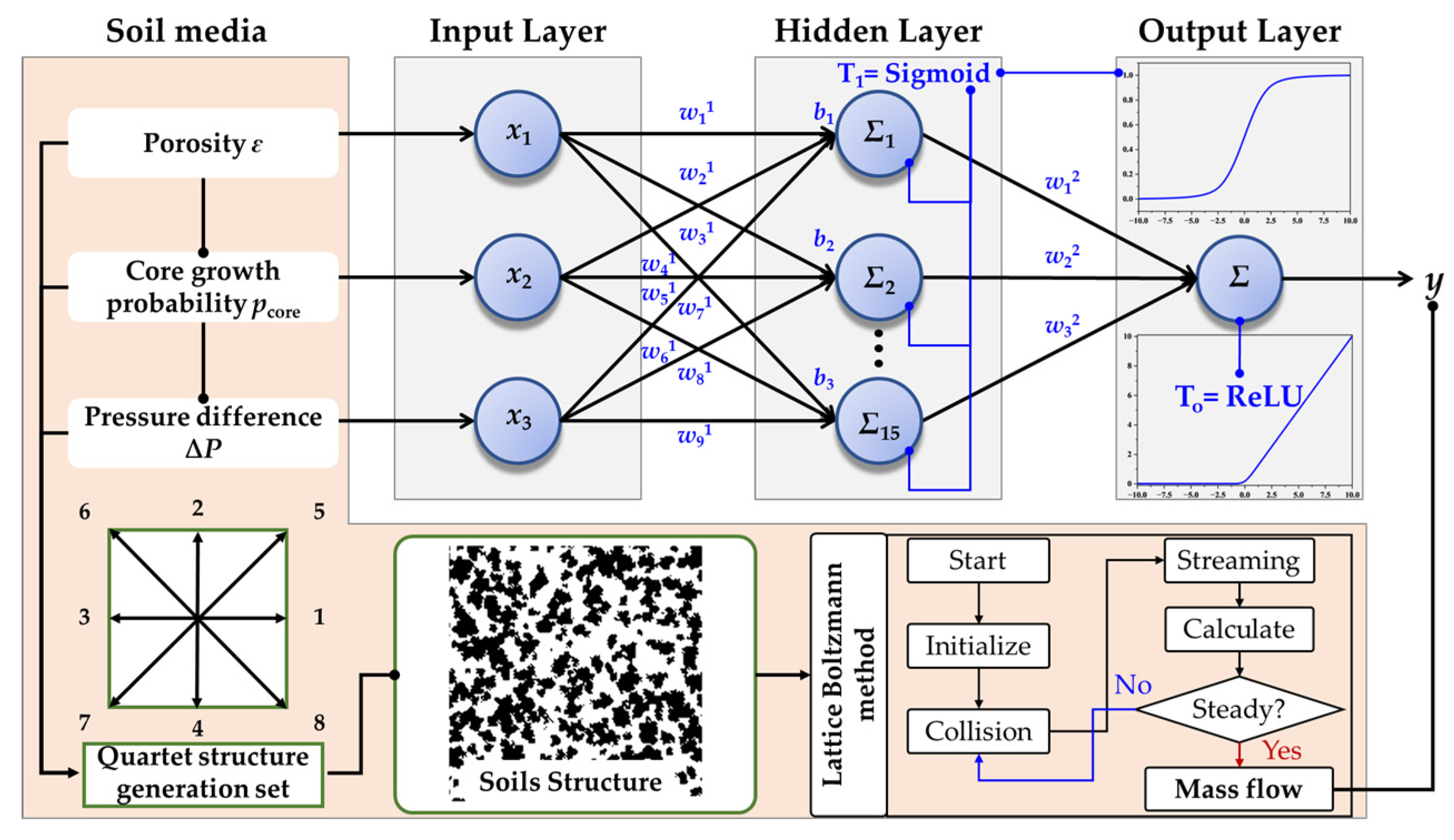
Figure 2: The structure of the established deep learning model and flow chart of the training.

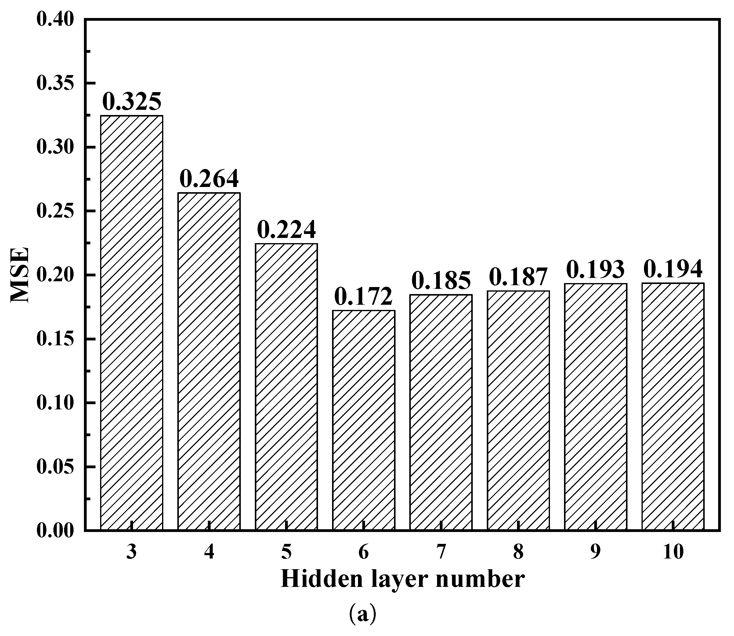
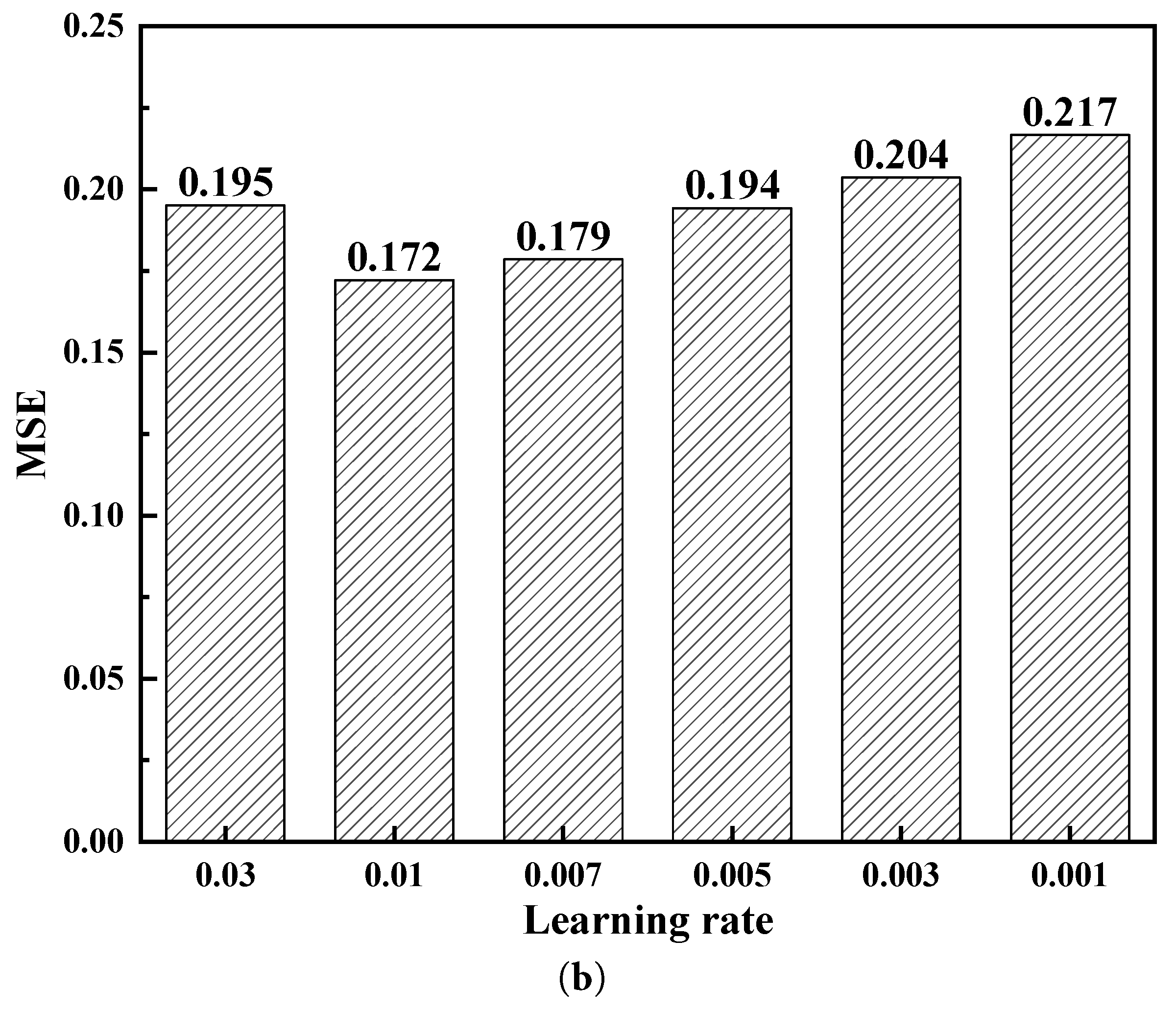
Figure 3: The hyperparameter optimization for hidden layer number (a) and learning rate (b).

2.4 Validation Strategy

The laminar flow of a fully developed incompressible Newtonian fluid in a long straight circular pipe has an exact analytical solution, namely the Poiseuille flow solution. Under a constant pressure gradient, the velocity profile follows a parabolic distribution along the radial direction, expressed as [54]: ux(y)=ΔP2μy(D−y)(6) where y denotes the vertical position from the centerline, Δ P is the pressure difference between inlet and outlet, μ represents the dynamic viscosity and D is the tube diameter. In this study, a computational domain with a size of 49 × 200 was designed, as shown in Fig. 4a. The availability of an analytical solution makes Poiseuille flow an ideal benchmark for validating numerical methods in computational fluid dynamics under constant pressure boundary conditions. By quantitatively comparing the velocity obtained from numerical simulation with analytical solution, the accuracy of the numerical algorithm in solving the Navier-Stokes equation under constant pressure boundary conditions can be effectively evaluated. In particular, the Poiseuille flow test provides a direct and rigorous means to verify the correct implementation of the pressure boundary condition and the proper coupling between pressure and velocity fields, thereby enhancing the credibility of the numerical results. As shown in Fig. 4b, the numerical results agree well with the analytical solution, confirming the accuracy of the present model.

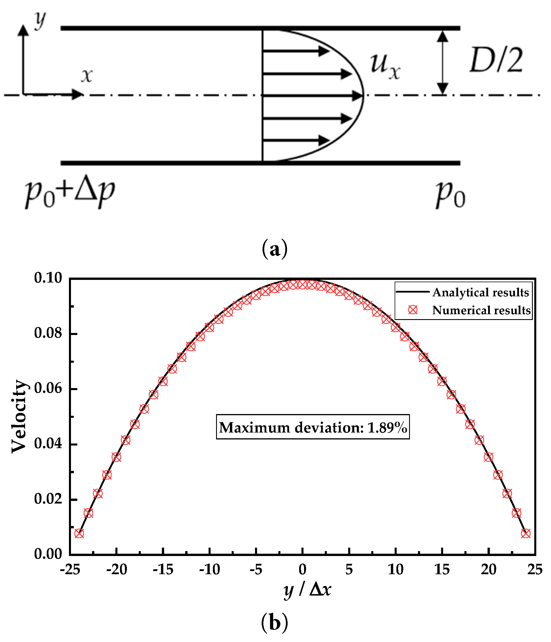
Figure 4: Schematic diagram of the calculation model (a) and comparison chart of result verification (b).

3 Data Reduction

After establishing the model, it is necessary to verify its accuracy. In addition, it is necessary to introduce the processing methods of the data studied in the research to enable readers to understand better.

This study mainly explores the influencing factors of seepage flow and the establishment of its deep learning prediction model. Seepage flow is simulated using a mesoscopic-scale flow model, with the primary parameter of interest being the mass flow rate. The mass flow rate, defined as the mass of fluid passing through a unit cross-sectional area per unit time, is of considerable practical importance in the study of porous media seepage. Compared to permeability, this parameter more directly reflects the actual flow capacity under specific operating conditions. The corresponding calculation formula is: F=∑iLxρu(7) where u and ρ are the velocity and density at the outlet, respectively, and the Lx represents the length of the outlet.

To evaluate prediction accuracy of deep learning model, commonly used RMSE, correlation coefficient R, average relative deviation ARD and mean error are employed [55].

Correlation coefficient (R):

Root mean square error (RMSE):

Average relative deviation (ARD):

Error mean:

4 Results and Discussions

This study mainly focuses on the seepage characteristics of porous media and establishes a deep learning prediction model. Employing the QSGS algorithm for stochastic generation of porous structures and the lattice Boltzmann method for mesoscopic flow simulation, the model’s performance is evaluated through comparisons on both training and independent prediction datasets.

4.1 The Influence of the Porosity

4.1.1 The Effect of the Porosity on the Flow

Porosity is a fundamental parameter that significantly influences the seepage process and its outcomes. Therefore, this study first conducts a comparative study on the seepage mass flow rates of the generated porous media with different porosities. The results are shown in Fig. 5. As porosity gradually increases, the seepage flow rate gradually increases. This trend can be explained theoretically: at lower porosities, the pore space within the porous medium is limited, resulting in higher flow resistance and a lower seepage mass flow rate. As the porosity gradually increases, the pressure difference that seepage needs to overcome becomes smaller, and the mass flow rate of seepage will also become larger. This phenomenon has also been revealed in the literature [56,57]. As the porosity gradual increases, the increasement of seepage mass flow rate also gradually increases. Since the vertical coordinate in the figure is a logarithmic coordinate, the increase in seepage mass flow rate becomes larger and larger with the increase in porosity. When the porosity is at a relatively low level, it increases from 0.60 to 0.65, and the seepage mass flow rate increases from 0.19 to 0.26, with an increase of 36.82%. When the porosity is at a relatively high level and increases from 0.90 to 0.95, the seepage mass flow rate increases from 5.32 to 15.22, with an increase of 186.09%. To further explore the influence of porosity on porous media, Fig. 5b analyzes the average pore size of the random porous media. The average pore size is another key descriptor of porous structures. As porosity increases, the average pore size also increases, and the rate of this increase accelerates. For instance, when porosity increases from 0.55 to 0.60, the average pore diameter increases from 6.36 to 7.62, a growth of 19.81%. However, when porosity increases from 0.90 to 0.95, the average pore diameter increases from 26.89 to 45.40, a much larger relative increase of 68.84%.

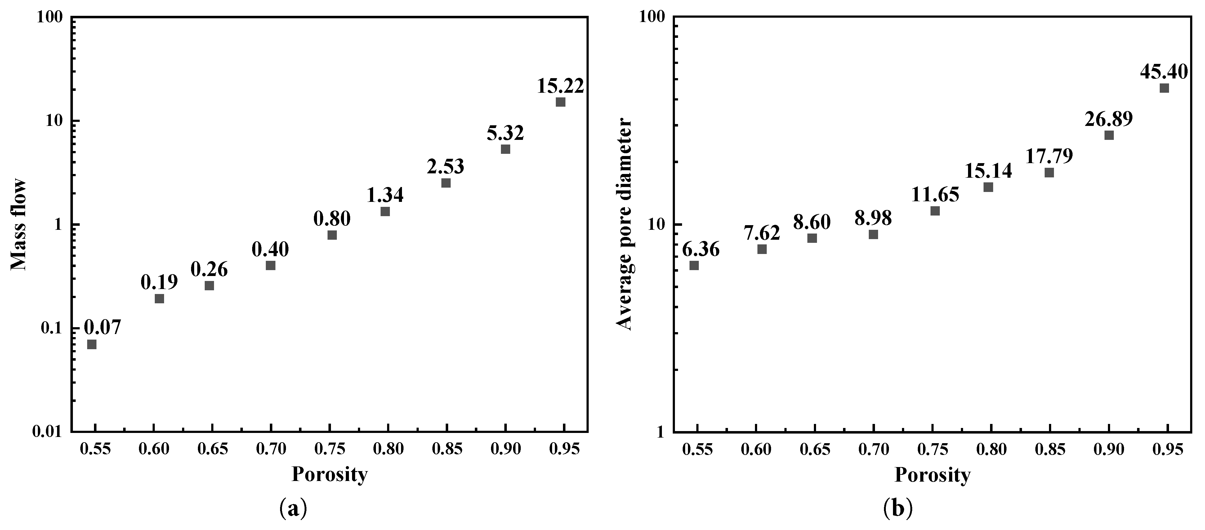
Figure 5: The influence of the porosity on the mass flow (a) and average pore diameter (b).

4.1.2 The Effect of the Porosity on the Streamlines

Fig. 6 compares the seepage flow diagrams of four porosities of 0.55, 0.65, 0.75, and 0.85. When the porosity is 0.55, the generated porous medium contains a relatively large number of dispersed solid blocks, resulting in a smaller average pore size. This increases the frictional resistance encountered by the fluid during flow. As the porosity gradually increases, the number of solid blocks decreases, leading to a larger average pore size and reduced flow resistance. Therefore, the velocity of the internal fluid flow will also increase. A comparison of the flow fields clearly shows that the highest fluid velocity occurs in the porous medium with a porosity of 0.85, while the lowest velocity is observed at a porosity of 0.55. As the porosity gradually decreases from 0.85 to 0.55, the flow velocity of the seepage gradually decreases. By choosing a porous medium with a certain porosity to conduct the analysis of fluid flow velocity, it can be found that when the fluid passes through the porous medium and the pore size changes from large to small, the flow velocity will increase, and the flow lines will become denser. This phenomenon is consistent with the Bernoulli equation, that is, a reduction in flow cross-sectional area results in an increase in velocity to maintain mass conservation for a constant mass flow rate.

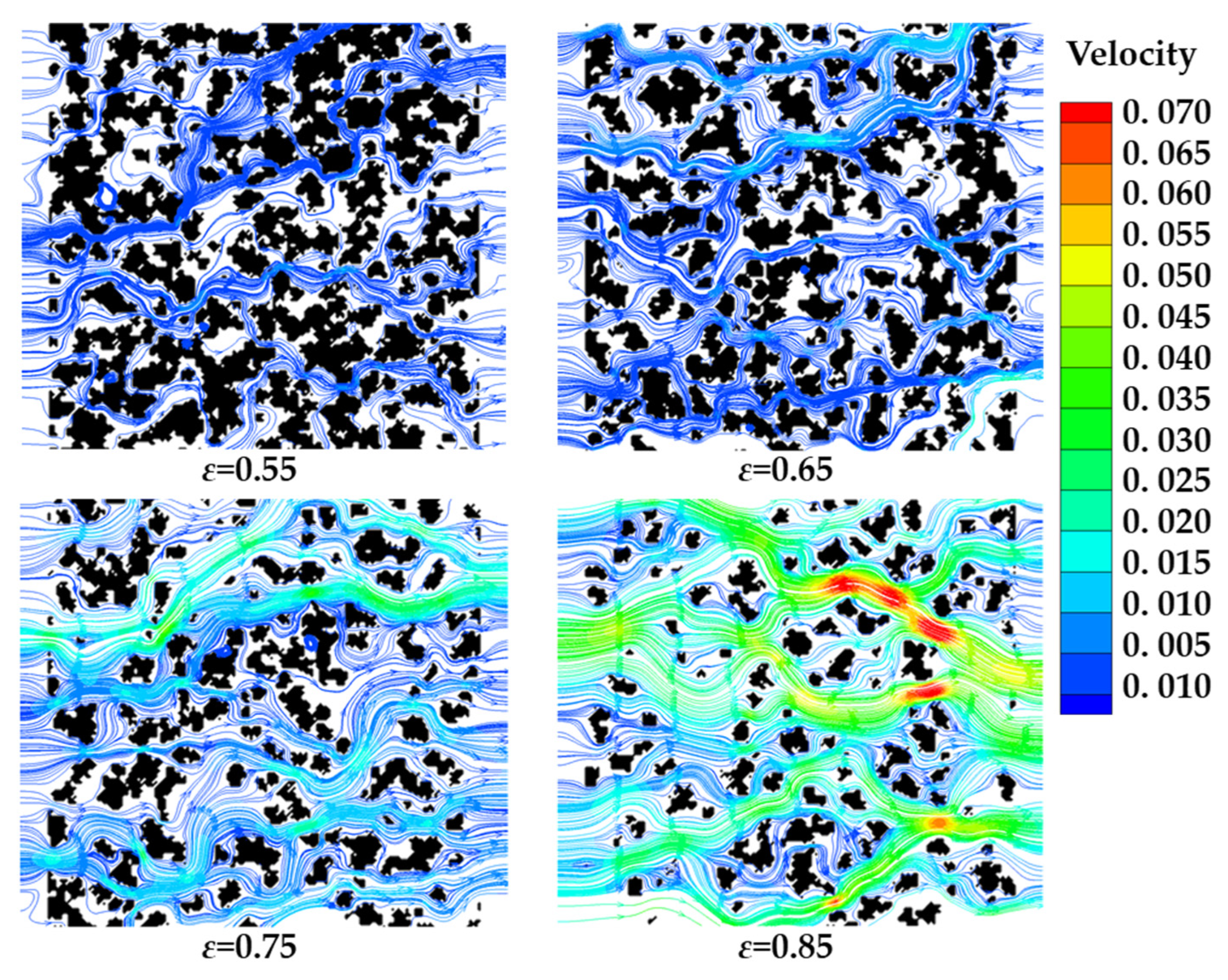
Figure 6: The streamlines of seepage in porous media with different porosities.

4.1.3 The Effect of the Porosity on the Pressure Distribution

Fig. 7 compares the pressure distributions for four porosities of 0.55, 0.65, 0.75, and 0.85 under constant pressure. It can be found from the figure that for different porosities, the pressure will continuously decrease as the fluid flows. Furthermore, the pressure drops more rapidly in media with smaller pores and denser solid matrices. For the position of the pore throat of porous media, since the seepage fluid consumes a large amount of pressure potential energy when passing through the narrow pore throat, this also leads to a significant pressure drop. For the positions of porous media with larger pores, the pressure consumed by internal seepage is relatively small. Therefore, the pressure drop at these positions is extremely low, and the pressure of the fluid still maintains a relatively high level. By observing the cloud map of the seepage pressure distribution in porous medium with a porosity of 0.85, the pressure remains high in the early flow region due to the sparse solid structure and correspondingly low flow resistance.

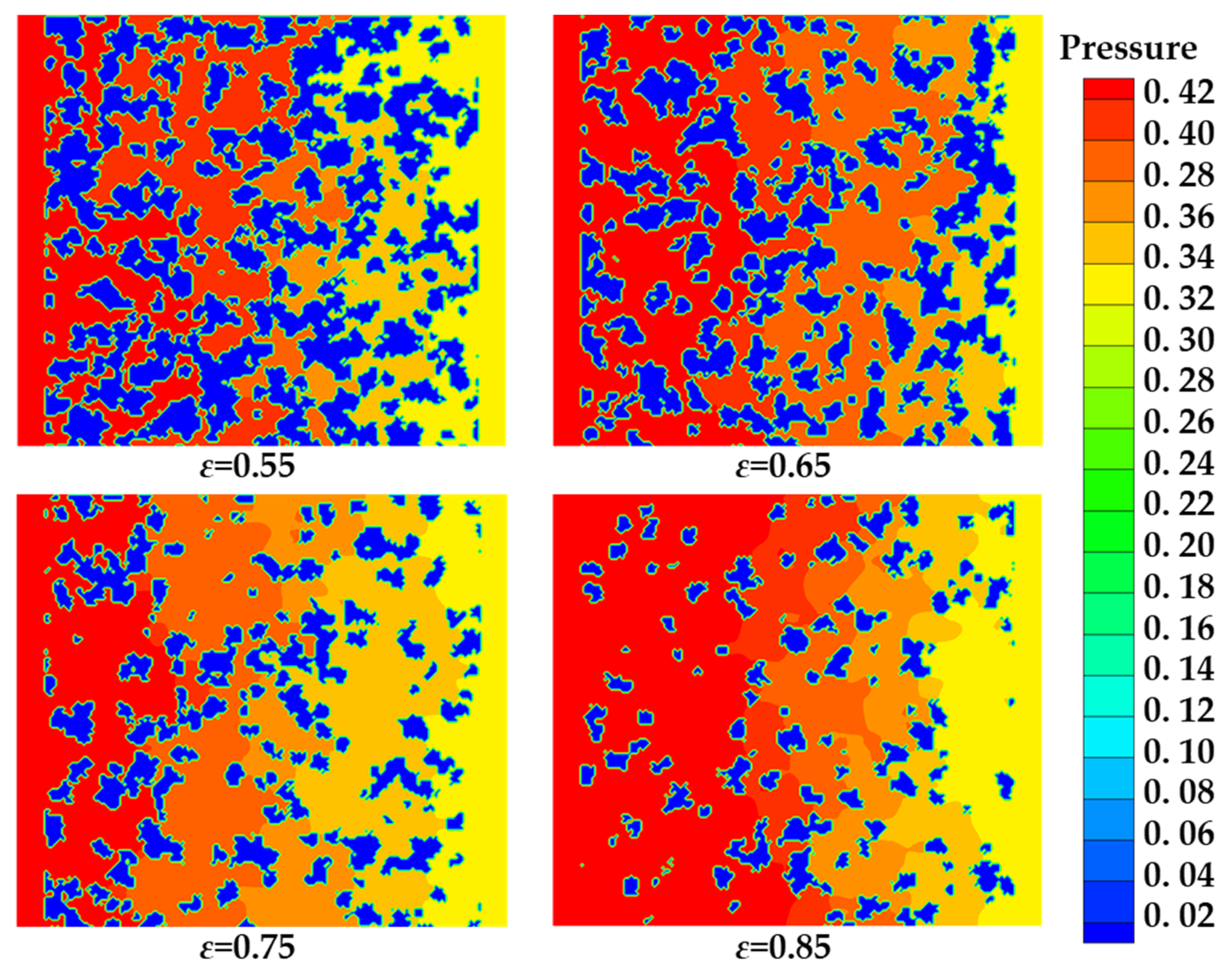
Figure 7: The pressure distribution in porous media with different porosities.

4.2 The Influence of the p_core

4.2.1 The Effect of the Porosity on the Pressure Distribution

In the process of generating porous media by QSGS, there are two control parameters, namely porosity and core growth probability, respectively. The core growth probability significantly influences the resulting porous structure by determining the initial number of nucleation sites, which in turn affects the number of solid aggregates. The overall manifestation is that the larger the core growth probability pcore is, the more blocks the generated porous medium has, the more dispersed the solid blocks of the porous medium are, and the smaller the average pore diameter of the generated porous medium is. Fig. 8a compares the seepage mass flow of the porous medium with a porosity of 0.55 controlled by the core growth probabilities of 0.001, 0.005, 0.05, 0.1, 0.5, and 0.9, respectively. The gradual increase of the core growth probability leads to a gradual decrease in the seepage mass flow rate of the porous medium, and the change ratio in the figure is nearly a linear change. However, the logarithmic vertical scale indicates that the rate of decrease diminishes at higher values of pcore. When the core growth probability was at a relatively low level, the change from 0.001 to 0.005 led to a decrease in the mass flow rate of the porous medium from 3.280 to 0.409, resulting in a reduction of 87.53%. When the core growth probability is at a relatively high level and increases from 0.500 to 0.900, the seepage mass flow rate of the porous medium decreases from 0.026 to 0.017, which leads to a decrease of 40.74%. According to the QSGS generation mechanism, variations in pcore also affect the average pore size of the porous medium. As shown in Fig. 8b, the average pore diameter gradually decreases as pcore increases, with the magnitude of reduction becoming smaller at higher probability levels. A comparison of Fig. 8a,b reveals that the seepage mass flow rate and the average pore diameter exhibit similar trends in response to changes in the core growth probability.

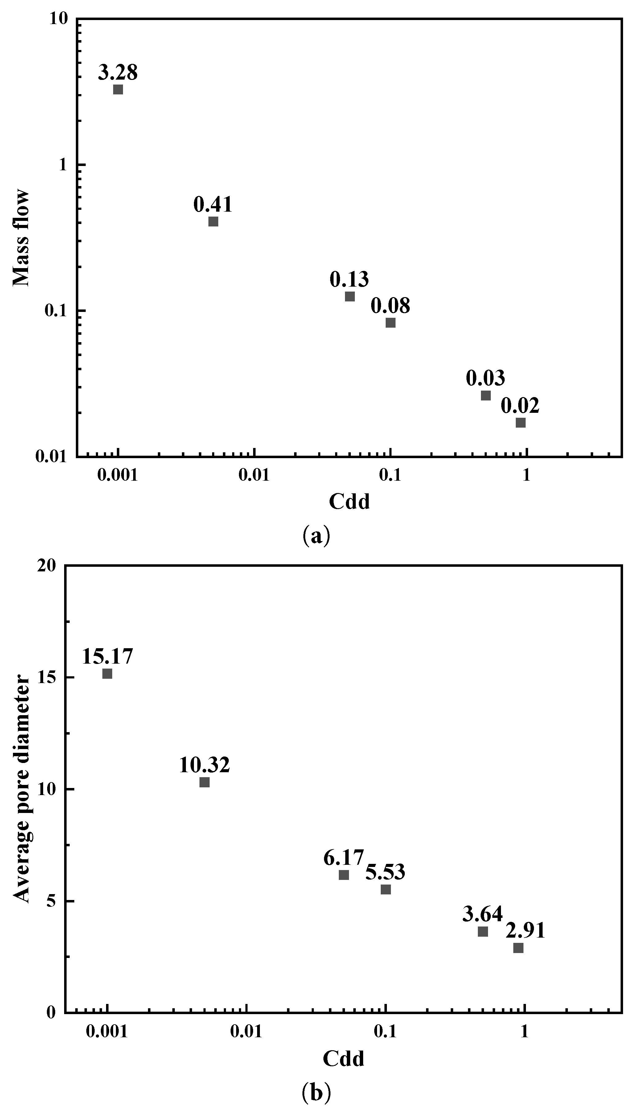
Figure 8: The influence of the probability of the core growth on the mass flow (a) and average pore diameter (b).

4.2.2 The Effect of the p_core on the Streamline

Fig. 9 compares the seepage flow in six porous media generated with core growth probabilities pcore of 0.001, 0.005, 0.05, 0.1, 0.5, and 0.9, respectively. While all six structures share the same porosity, they differ significantly in pore size distribution. When the core growth probability is low, the generated porous medium has a high pore size distribution. When the porous medium has a large core growth probability, the generated porous medium has a low pore size distribution. Therefore, when the core growth probability is 0.001, the porous medium has the largest pore size distribution and also the largest fluid velocity. As the core growth probability gradually increases, the pore size becomes smaller and smaller, and the flow velocity of the internal fluid also becomes smaller and smaller. When pcore ≥ 0.5, the solid phase becomes highly dispersed, resembling isolated particles, which significantly increases flow resistance and results in an extremely low internal fluid velocity.

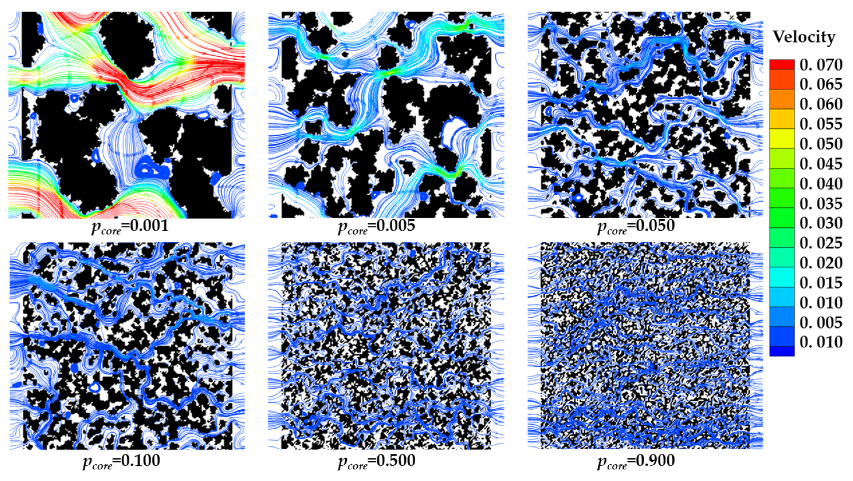
Figure 9: The streamlines of seepage in porous media with different probabilities of the core growth.

4.2.3 The Effect of the p_core on the Pressure Distribution

Fig. 10 compares the seepage pressure distributions in six porous media corresponding to the core growth probabilities pcore of 0.001, 0.005, 0.050, 0.100, 0.500, and 0.900, respectively. In the case where pcore = 0.001, the pore structure exhibits a clear influence of pore throats on the pressure distribution. The upstream region, characterized by relatively large pores, shows minimal pressure loss. However, a sharp pressure drop occurs as the fluid passes through a narrow pore throat. In contrast, for the porous medium generated with pcore = 0.900, the pressure decreases rapidly throughout the flow domain. This accelerated pressure loss is attributed to the highly dispersed solid phase, which significantly increases flow resistance and dissipates pressure more quickly.

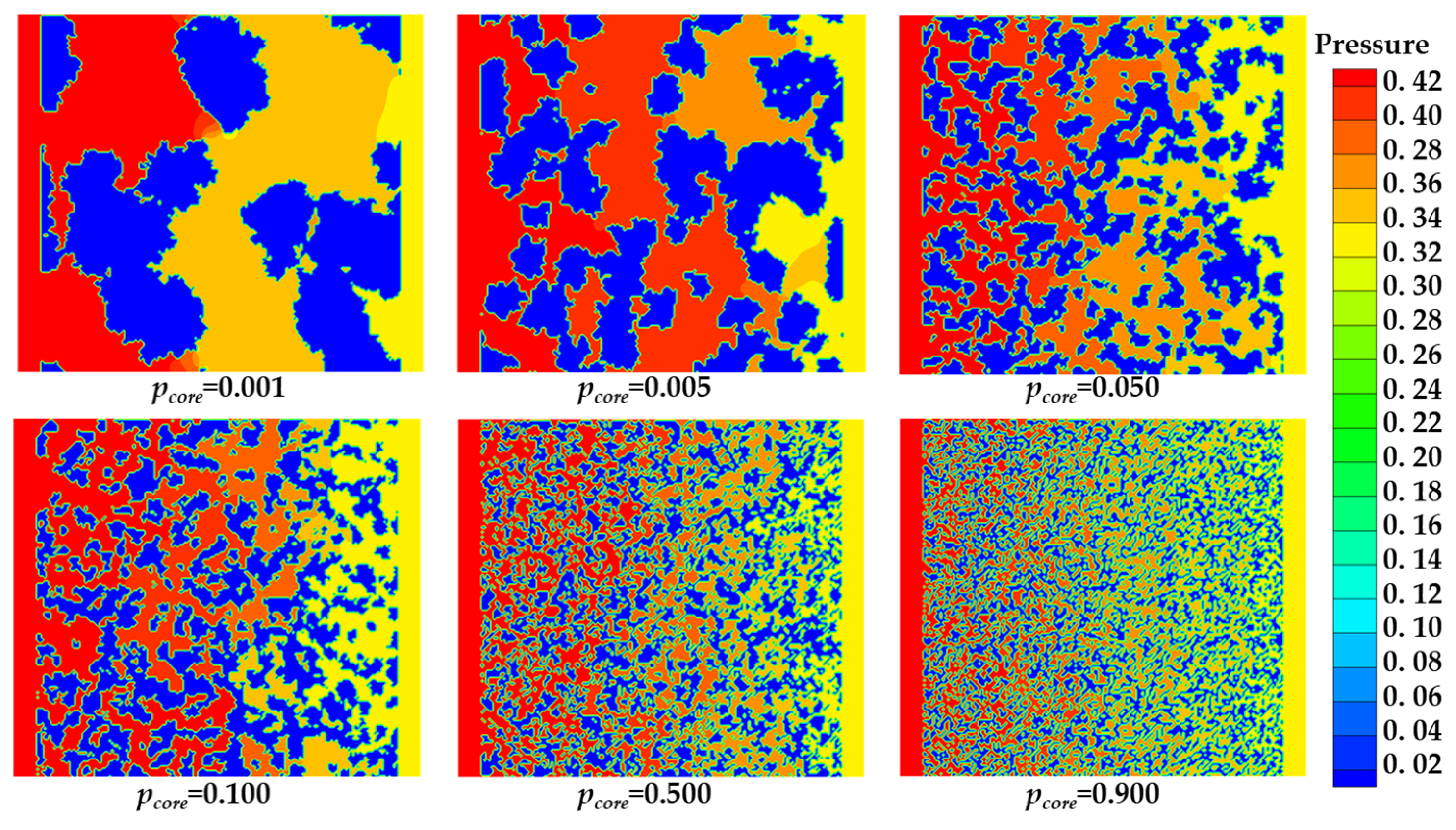
Figure 10: The pressure distribution in porous media with different probabilities of the core growth.

4.3 The Influence of the Pressure Difference and Dynamic Viscosity

Seepage pressure provides the driving force for fluid flow, while dynamic viscosity represents the flow resistance, and both parameters directly influence the seepage mass flow rate. To explore the effect of pressure differences and different hydrodynamic viscosities on the seepage of porous media, this section uses the established seepage model of porous media to calculate the seepage mass under different hydrodynamic viscosities under different pressure differences. The porous medium considered in this section has a porosity of 0.55. To isolate the individual effects of each parameter, the same porous structure was used across all simulations. The research results are shown in Fig. 11. For a given dynamic viscosity, the seepage mass flow rate increases linearly with the applied pressure difference. This behavior is consistent with Darcy’s law, which states that the flow rate is proportional to the pressure gradient. Conversely, under a fixed pressure difference, the seepage mass flow rate decreases as the dynamic viscosity increases, a trend also reported in reference [58]. The reduction in flow rate is more pronounced at lower viscosity levels. Overall, regardless of the fluid viscosity, the seepage mass flow rate exhibits a proportional relationship with the pressure difference.

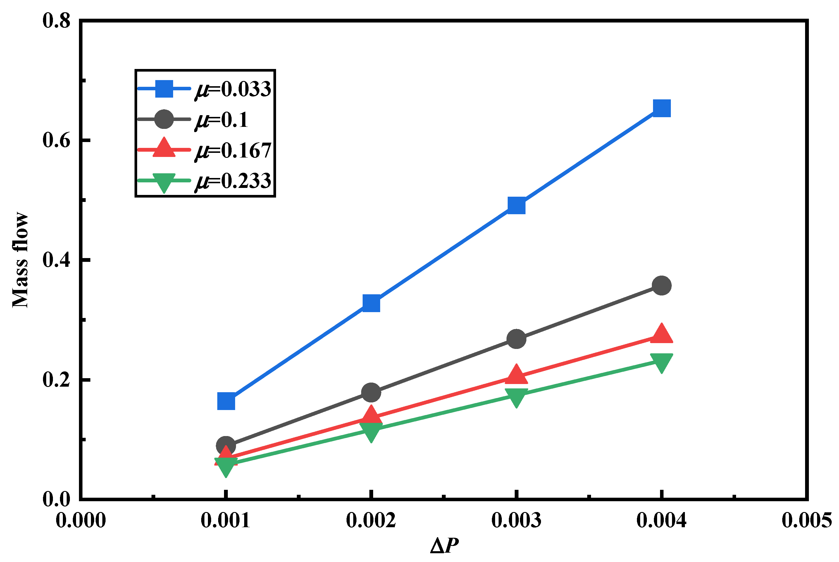
Figure 11: The mass flow of seepage of fluid under different pressure differences.

4.4 The Prediction Results of Trained Model

Based on a dataset comprising various porous media structures generated via the QSGS method and their corresponding seepage mass flow rates computed by the LBM, a deep learning model was trained to accurately predict seepage flow behavior. Unlike the image-based CNN approaches commonly adopted in previous studies, this work adopts a feature-based strategy using statistical control parameters. The control parameters of the porous media, porosity and the core growth probability pcore, were taken as the input parameters of the training model. At the same time, the applied pressure difference, which strongly influences the seepage process, was also taken as an input parameter. The seepage mass flow rate calculated by LBM is taken as the predicted value of the model to train the established deep learning model.

Based on the QSGS-generated porous media analogous to soil structures in terms of pore scale, this study selected a porosity range of 0.55–0.75, representative of typical soil-based porous media. Since different soil types can lead to inconsistent agglomeration sizes of soil-like porous media, thereby generating different pore sizes. The core growth probability in QSGS was varied between 0.01 and 0.07 to account for variations in pore size. The applied pressure difference given in this study is from 0.001 to 0.004. Within the range of this independent variable, 176 groups of porous media were formed. Due to the stochastic nature of QSGS in generating porous media, two realizations were produced for each parameter set. The average seepage mass flow from these two realizations was used as the target output for model training, resulting in a total training dataset of 352 samples. While Sudakov et al. [49] used 9261 samples to train; Zhang et al. [50] used 25,000 as training data set. Compared with their work, which is conducted through image-based prediction method, the training dataset is greatly saved and a relatively good accuracy is gained. Fig. 12a depicts the prediction results of the trained model on the training dataset. The results indicate that the trained model can predict all points well, and the prediction errors are almost all within the range of ±80%. A more detailed view in Fig. 12b indicates that nearly all predictions lie within ±20% of the true values. There is a point in the study where the prediction deviation exceeds 20%. This might be because the two results of the random porous media generated by QSGS under this set of parameters are exactly very similar, failing to effectively eliminate the influence of the randomly generated porous media by the QSGS method. Overall, the model demonstrates a strong ability to accurately predict seepage mass flow rates for QSGS-generated porous media under different applied pressure difference.

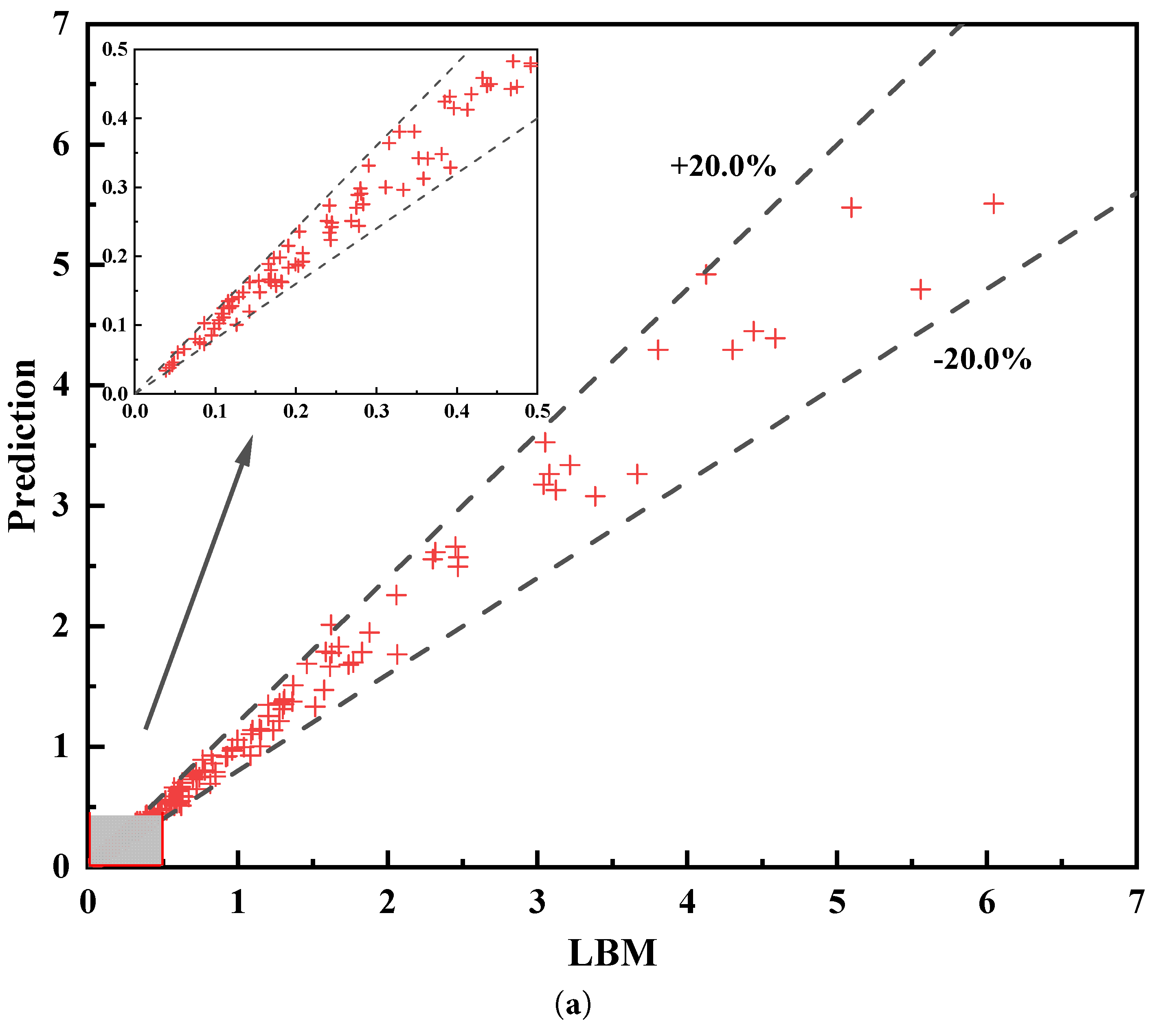
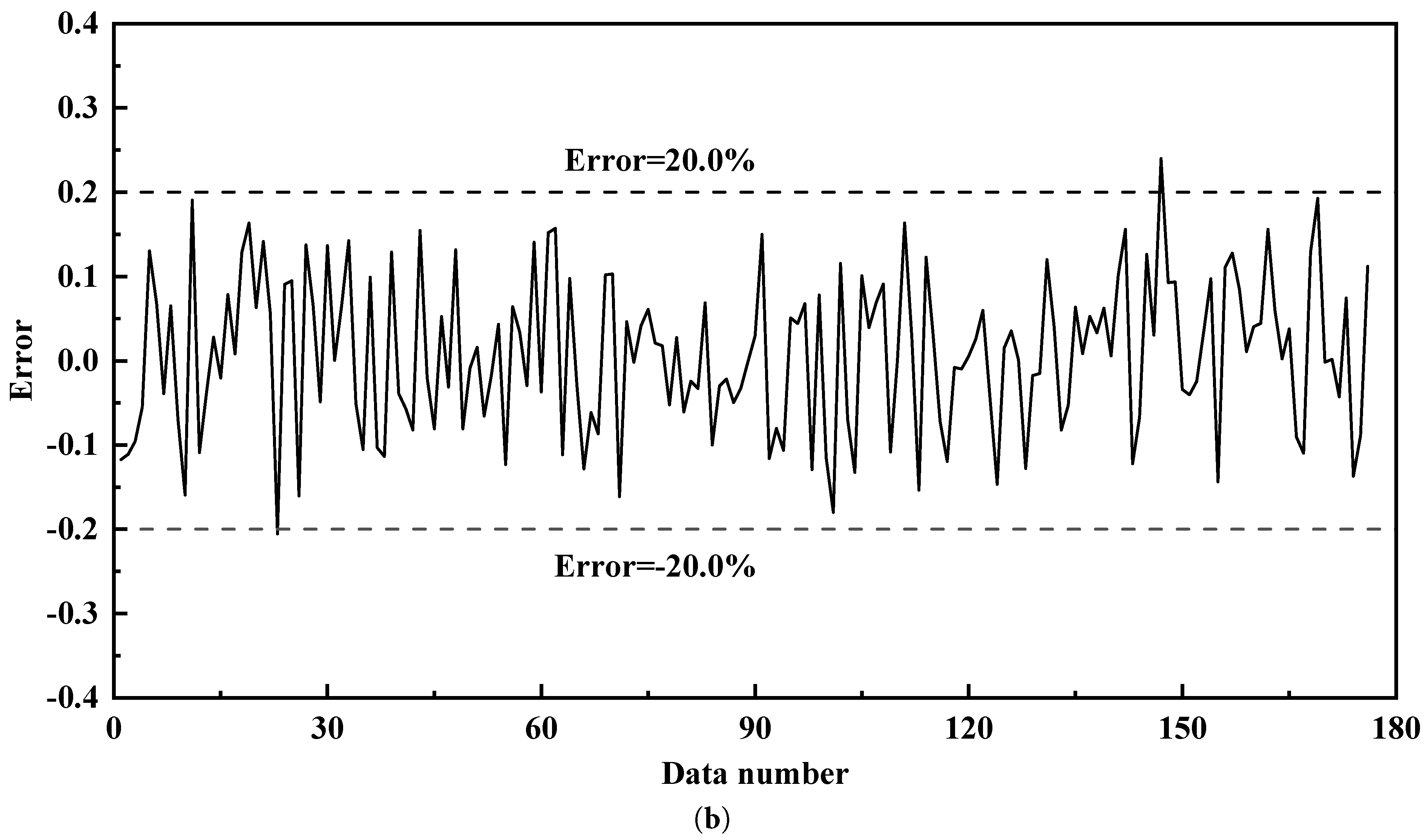
Figure 12: The prediction results (a) and relative error of training dataset (b).

After training the deep learning model, 30 additional samples generated by QSGS were calculated to evaluate prediction accuracy. Fig. 13 shows the comparison between predicted and actual seepage mass flow rates for the test dataset. The trained model can achieve very good prediction accuracy for predicting the test dataset, with all data points falling within an error range of ±20%. A quantitative assessment of the model performance is summarized in Table 1, which includes the correlation coefficient, root mean square error, average relative deviation and mean error. The model achieves a correlation coefficient R of 0.98558, indicating a strong relationship between the input parameters, porosity, core growth probability, applied pressure difference and the seepage mass flow rate. The root means square error is 0.24261, which proves that the predicted values are very close to the actual values and the deviation is small. The average relative deviation is 0.14645, which also proves that the average deviation of all prediction points is acceptable. Furthermore, the average error of –0.02197, being close to zero under an ARD of 0.14645, indicates that the errors are evenly distributed and do not exhibit significant systematic bias, consistent with a roughly normal distribution of prediction errors.

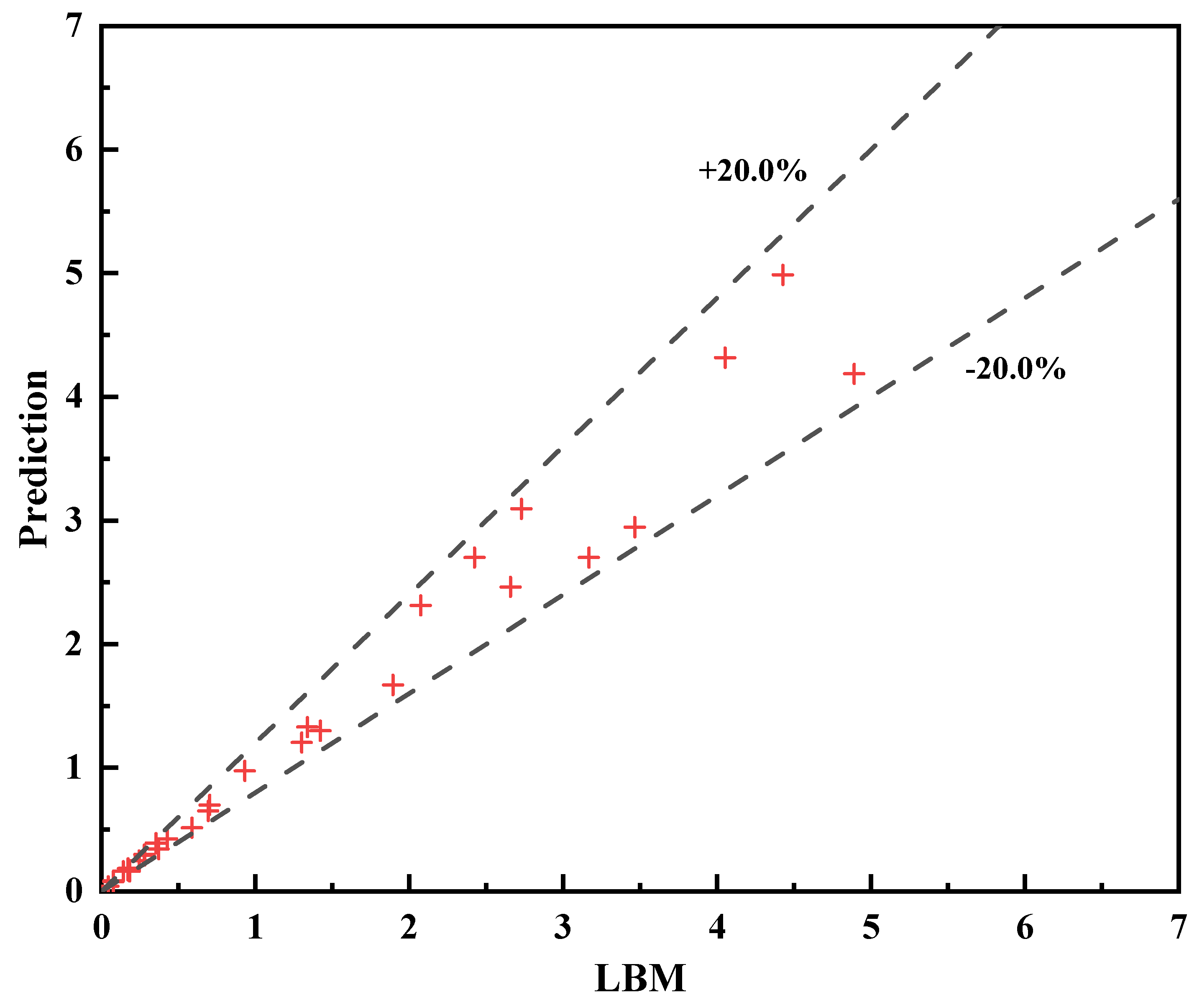
Figure 13: The prediction results of testing dataset.

5 Conclusions

In this study, soil-like porous media was generated using the QSGS method. The seepage mass flow rate was then computed via a mesoscopic numerical model, and the results were employed as input-output pairs to train a deep learning model for rapid seepage prediction. The following conclusions were obtained during the research process.

• 1.Porosity and core growth probability significantly influence the average pore diameter and seepage mass flow rate. Higher porosity and core growth probability result in larger average pore sizes and greater seepage flow. Moreover, the influence amplitudes of changing porosity and core growth probability on mass flow rate decrease with the increase of the two parameters.
• 2.Flow velocity is higher in regions with larger pore diameters, where pressure loss remains relatively small. In contrast, significant pressure drops occur at pore throats or constricted regions.
• 3.As applied pressure differences increase, the seepage flow rate exhibits a proportional rise for a given fluid. Conversely, higher dynamic viscosity of the fluid leads to a reduction in the seepage flow rate under the same pressure conditions.
• 4.The deep learning model based on full-numerical transfer achieved satisfactory predictive accuracy for the seepage mass flow rate, with a root mean square error of 0.24261 and a mean error of −0.02197.

It should be noted that this research proposes a new seepage prediction approach suitable for situations with limited training data. At this circumstance, the present method is better than that using image-based deep learning model. However, when ample training data are available, image-based deep learning models may yield better performance. Furthermore, to save time for calculating a large amount of training data, it is suggested to incorporate the GPU-accelerated parallel numerical simulations.

References

1. Ahadiyan J , Bahmanpouri F , Adeli A , Gualtieri C , Khoshkonesh A . Riprap effect on hydraulic fracturing process of cohesive and non-cohesive protective levees. Water Resour Manage. 2022; 36( 2): 625– 39. doi:10.1007/s11269-021-03044-6. [Google Scholar] [CrossRef]
2. Poursaki R , Ahadian J , Seraj M . A 3D mathematical modeling in solving analytical consolidation equation in a homogeneous saturated soil. J Adv Math Model. 2015; 5: 59– 74. [Google Scholar]
3. Peng S , Zhang H , Chai C , Xue S , Zhang X . Effects of soil properties on the diffusion of hydrogen-blended natural gas from an underground pipe. Fluid Dyn Mater Process. 2025; 21( 5): 1099– 112. doi:10.32604/fdmp.2025.060452. [Google Scholar] [CrossRef]
4. Aggelopoulos CA , Tsakiroglou CD . The effect of micro-heterogeneity and capillary number on capillary pressure and relative permeability curves of soils. Geoderma. 2008; 148( 1): 25– 34. doi:10.1016/j.geoderma.2008.08.011. [Google Scholar] [CrossRef]
5. Liu YF , Jeng DS . Pore scale study of the influence of particle geometry on soil permeability. Adv Water Resour. 2019; 129: 232– 49. doi:10.1016/j.advwatres.2019.05.024. [Google Scholar] [CrossRef]
6. Kumar P , Rao B , Burman A , Kumar S , Samui P . Spatial variation of permeability and consolidation behaviors of soil using ordinary Kriging method. Groundw Sustain Dev. 2023; 20: 100856. doi:10.1016/j.gsd.2022.100856. [Google Scholar] [CrossRef]
7. Wang P , Zhang X . Experimental study on seepage characteristics of a soil-rock mixture in a fault zone. Fluid Dyn Mater Process. 2022; 18( 2): 271– 83. doi:10.32604/fdmp.2022.017882. [Google Scholar] [CrossRef]
8. Germanou L , Ho MT , Zhang Y , Wu L . Intrinsic and apparent gas permeability of heterogeneous and anisotropic ultra-tight porous media. J Nat Gas Sci Eng. 2018; 60: 271– 83. doi:10.1016/j.jngse.2018.10.003. [Google Scholar] [CrossRef]
9. Shams R , Masihi M , Boozarjomehry RB , Blunt MJ . A hybrid of statistical and conditional generative adversarial neural network approaches for reconstruction of 3D porous media (ST-CGAN). Adv Water Resour. 2021; 158: 104064. doi:10.1016/j.advwatres.2021.104064. [Google Scholar] [CrossRef]
10. Tahmasebi P , Javadpour F , Sahimi M . Multiscale and multiresolution modeling of shales and their flow and morphological properties. Sci Rep. 2015; 5: 16373. doi:10.1038/srep16373. [Google Scholar] [CrossRef]
11. Liu P , Nie B , Zhao Z , Li J , Yang H , Qin C . Permeability of micro-scale structure in coal: insights from μ-CT image and pore network modelling. Gas Sci Eng. 2023; 111: 204931. doi:10.1016/j.jgsce.2023.204931. [Google Scholar] [CrossRef]
12. Eshghinejadfard A , Daróczy L , Janiga G , Thévenin D . Calculation of the permeability in porous media using the lattice Boltzmann method. Int J Heat Fluid Flow. 2016; 62: 93– 103. doi:10.1016/j.ijheatfluidflow.2016.05.010. [Google Scholar] [CrossRef]
13. Zakirov T , Galeev A . Absolute permeability calculations in micro-computed tomography models of sandstones by Navier-Stokes and lattice Boltzmann equations. Int J Heat Mass Transf. 2019; 129: 415– 26. doi:10.1016/j.ijheatmasstransfer.2018.09.119. [Google Scholar] [CrossRef]
14. Wang J , Kang Q , Wang Y , Pawar R , Rahman SS . Simulation of gas flow in micro-porous media with the regularized lattice Boltzmann method. Fuel. 2017; 205: 232– 46. doi:10.1016/j.fuel.2017.05.080. [Google Scholar] [CrossRef]
15. Luo Y , Li W , Huang F . Permeability model of fracture network based on branch length distribution and topological connectivity. Phys Fluids. 2023; 35( 8): 083601. doi:10.1063/5.0160043. [Google Scholar] [CrossRef]
16. Zdravkovic L , Carter J . Contributions to Géotechnique 1948–2008: constitutive and numerical modelling. Géotechnique. 2008; 58( 5): 405– 12. doi:10.1680/geot.2008.58.5.405. [Google Scholar] [CrossRef]
17. Xia H , Lai Y , Mousavi-Nezhad M . Meso-scale investigation on the permeability of frozen soils with the lattice Boltzmann method. Phys Fluids. 2024; 36( 9): 093616. doi:10.1063/5.0222658. [Google Scholar] [CrossRef]
18. Wang M , Wang J , Pan N , Chen S . Mesoscopic predictions of the effective thermal conductivity for microscale random porous media. Phys Rev E. 2007; 75( 3): 036702. doi:10.1103/physreve.75.036702. [Google Scholar] [CrossRef]
19. Pu Y , Ma P , Chen H , Li D , Arıcı M . Characterization investigation on pore-resistance relationship of oil contaminants in soil porous structure. J Petrol Sci Eng. 2020; 191: 107208. doi:10.1016/j.petrol.2020.107208. [Google Scholar] [CrossRef]
20. Øren PE , Bakke S . Process based reconstruction of sandstones and prediction of transport properties. Transp Porous Medium. 2002; 46( 2): 311– 43. doi:10.1023/A:1015031122338. [Google Scholar] [CrossRef]
21. Wu K , Nunan N , Crawford JW , Young IM , Ritz K . An efficient Markov chain model for the simulation of heterogeneous soil structure. Soil Sci Soc Am J. 2004; 68( 2): 346. doi:10.2136/sssaj2004.3460. [Google Scholar] [CrossRef]
22. Hazlett RD . Simulation of capillary-dominated displacements in microtomographic images of reservoir rocks. Transp Porous Medium. 1995; 20( 1): 21– 35. doi:10.1007/BF00616924. [Google Scholar] [CrossRef]
23. Wang Z , Jin X , Wang X , Sun L , Wang M . Pore-scale geometry effects on gas permeability in shale. J Nat Gas Sci Eng. 2016; 34: 948– 57. doi:10.1016/j.jngse.2016.07.057. [Google Scholar] [CrossRef]
24. Zhou XP , Xiao N . 3D numerical reconstruction of porous sandstone using improved simulated annealing algorithms. Rock Mech Rock Eng. 2018; 51( 7): 2135– 51. doi:10.1007/s00603-018-1451-z. [Google Scholar] [CrossRef]
25. Yang G , Liu T , Lu X , Wang M . Fast-QSGS: a GPU accelerated program for structure generation of granular disordered media. Comput Phys Commun. 2024; 302: 109241. doi:10.1016/j.cpc.2024.109241. [Google Scholar] [CrossRef]
26. Li T , Li M , Jing X , Xiao W , Cui Q . Influence mechanism of pore-scale anisotropy and pore distribution heterogeneity on permeability of porous media. Petrol Explor Dev. 2019; 46( 3): 594– 604. doi:10.1016/S1876-3804(19)60039-X. [Google Scholar] [CrossRef]
27. Wu T , Yang Y , Wang Z , Shen Q , Tong Y , Wang M . Anion diffusion in compacted clays by pore-scale simulation and experiments. Water Resour Res. 2020; 56( 11): 1– 17. doi:10.1029/2019wr027037. [Google Scholar] [CrossRef]
28. Tian J , Qi C , Sun Y , Yaseen ZM . Surrogate permeability modelling of low-permeable rocks using convolutional neural networks. Comput Meth Appl Mech Eng. 2020; 366: 113103. doi:10.1016/j.cma.2020.113103. [Google Scholar] [CrossRef]
29. Chen L , Kang Q , Dai Z , Viswanathan HS , Tao W . Permeability prediction of shale matrix reconstructed using the elementary building block model. Fuel. 2015; 160: 346– 56. doi:10.1016/j.fuel.2015.07.070. [Google Scholar] [CrossRef]
30. Li Y , Huang X , Li Z , Xie Y , Yang X , Li MJ . Structural optimization of latent heat storage tank filled with nickel foam. Appl Therm Eng. 2025; 267: 125780. doi:10.1016/j.applthermaleng.2025.125780. [Google Scholar] [CrossRef]
31. Li Y , Xie Y , Gao J , Yang X , Sundén B . Solidification characteristics in rotating gradient metal foam based on Taguchi and response surface analysis. Int J Heat Mass Transf. 2025; 250: 127324. doi:10.1016/j.ijheatmasstransfer.2025.127324. [Google Scholar] [CrossRef]
32. Xu A , Shi L , Zhao TS . Accelerated lattice Boltzmann simulation using GPU and OpenACC with data management. Int J Heat Mass Transf. 2017; 109: 577– 88. doi:10.1016/j.ijheatmasstransfer.2017.02.032. [Google Scholar] [CrossRef]
33. Zhang T , Du Y , Huang T , Li X . GPU-accelerated 3D reconstruction of porous media using multiple-point statistics. Comput Geosci. 2015; 19( 1): 79– 98. doi:10.1007/s10596-014-9452-9. [Google Scholar] [CrossRef]
34. Tahmasebi P , Sahimi M , Mariethoz G , Hezarkhani A . Accelerating geostatistical simulations using graphics processing units (GPU). Comput Geosci. 2012; 46: 51– 9. doi:10.1016/j.cageo.2012.03.028. [Google Scholar] [CrossRef]
35. Wang Q , Li C , Zhao Y , Ai D . Study of gas emission law at the heading face in a coal-mine tunnel based on the lattice Boltzmann method. Energy Sci Eng. 2020; 8( 5): 1705– 15. doi:10.1002/ese3.626. [Google Scholar] [CrossRef]
36. Ren X , Guo Z , Ning F , Ma S . Permeability of hydrate-bearing sediments. Earth Sci Rev. 2020; 202: 103100. doi:10.1016/j.earscirev.2020.103100. [Google Scholar] [CrossRef]
37. Guo BE , Xiao N , Martyushev D , Zhao Z . Deep learning-based pore network generation: numerical insights into pore geometry effects on microstructural fluid flow behaviors of unconventional resources. Energy. 2024; 294: 130990. doi:10.1016/j.energy.2024.130990. [Google Scholar] [CrossRef]
38. Zhao Z , Zhou XP . A novel voxel-particle energy approach to predict 3D microscopic fracture surface of porous geomaterials and fracture permeability modeling. Eng Geol. 2023; 323: 107214. doi:10.1016/j.enggeo.2023.107214. [Google Scholar] [CrossRef]
39. Zhao Z , Zhou XP . A comprehensive review of various AI-based segmentation algorithms for multiscale rocks: principles, evaluations, simple applications and future directions. Rock Mech Rock Eng. 2025; 58( 9): 10541– 76. doi:10.1007/s00603-025-04651-0. [Google Scholar] [CrossRef]
40. Ahadiyan J . Application of ANFIS adaptive system to estimate the potential consolidation of clay soils. J Model Eng. 2016; 14: 17– 31. [Google Scholar]
41. Karimi M , Salemnia A , Ahadiyan J . Evaluation of strength parameters of stress-strain development in clay soil and clay-sand soil. Int J Civ Struct Eng. 2010; 1: 644– 60. [Google Scholar]
42. Ishola O , Vilcáez J . Machine learning modeling of permeability in 3D heterogeneous porous media using a novel stochastic pore-scale simulation approach. Fuel. 2022; 321: 124044. doi:10.1016/j.fuel.2022.124044. [Google Scholar] [CrossRef]
43. Menke HP , Maes J , Geiger S . Upscaling the porosity–permeability relationship of a microporous carbonate for Darcy-scale flow with machine learning. Sci Rep. 2021; 11: 2625. doi:10.1038/s41598-021-82029-2. [Google Scholar] [CrossRef]
44. Wu J , Yin X , Xiao H . Seeing permeability from images: fast prediction with convolutional neural networks. Sci Bull. 2018; 63( 18): 1215– 22. doi:10.1016/j.scib.2018.08.006. [Google Scholar] [CrossRef]
45. Alqahtani N , Alzubaidi F , Armstrong RT , Swietojanski P , Mostaghimi P . Machine learning for predicting properties of porous media from 2D X-ray images. J Petrol Sci Eng. 2020; 184: 106514. doi:10.1016/j.petrol.2019.106514. [Google Scholar] [CrossRef]
46. Tembely M , AlSumaiti A . Deep learning for a fast and accurate prediction of complex carbonate rock permeability from 3D micro-CT images. In: Proceedings of the Abu Dhabi International Petroleum Exhibition & Conference; 2019 Nov 11–14; Abu Dhabi, United Arab Emirates. doi:10.2118/197457-ms. [Google Scholar] [CrossRef]
47. Kamrava S , Tahmasebi P , Sahimi M . Linking morphology of porous media to their macroscopic permeability by deep learning. Transp Porous Med. 2020; 131( 2): 427– 48. doi:10.1007/s11242-019-01352-5. [Google Scholar] [CrossRef]
48. Liu S , Barati R , Zhang C . Fast estimation of permeability in sandstones by 3D convolutional neural networks. In: SEG technical program expanded abstracts 2019. San Antonio, TX, USA: Society of Exploration Geophysicists; 2019. p. 4833– 8. doi:10.1190/segam2019-3216569.1. [Google Scholar] [CrossRef]
49. Sudakov O , Burnaev E , Koroteev D . Driving digital rock towards machine learning: predicting permeability with gradient boosting and deep neural networks. Comput Geosci. 2019; 127: 91– 8. doi:10.1016/j.cageo.2019.02.002. [Google Scholar] [CrossRef]
50. Zhang H , Yu H , Yuan X , Xu H , Micheal M , Zhang J , et al. Permeability prediction of low-resolution porous media images using autoencoder-based convolutional neural network. J Petrol Sci Eng. 2022; 208: 109589. doi:10.1016/j.petrol.2021.109589. [Google Scholar] [CrossRef]
51. Guo Z , Zhao TS . Lattice Boltzmann model for incompressible flows through porous media. Phys Rev E. 2002; 66( 3): 036304. doi:10.1103/physreve.66.036304. [Google Scholar] [CrossRef]
52. Zou Q , He X . On pressure and velocity boundary conditions for the lattice Boltzmann BGK model. Phys Fluids. 1997; 9( 6): 1591– 8. doi:10.1063/1.869307. [Google Scholar] [CrossRef]
53. Krüger T , Kusumaatmaja H , Kuzmin A , Shardt O , Silva G , Viggen EM . The lattice Boltzmann method: principles and practice. Cham, Switzerland: Springer; 2017. doi:10.1007/978-3-319-44649-3. [Google Scholar] [CrossRef]
54. Liu W , Wu CY . Analysis of inertial migration of neutrally buoyant particle suspensions in a planar Poiseuille flow with a coupled lattice Boltzmann method-discrete element method. Phys Fluids. 2019; 31( 6): 063301. doi:10.1063/1.5095758. [Google Scholar] [CrossRef]
55. Li Y , Huang X , Yang X , Ai B , Chen S . Comparative study on deep learning prediction of directional thermal conductivity of anisotropic porous media. Int J Therm Sci. 2025; 212: 109759. doi:10.1016/j.ijthermalsci.2025.109759. [Google Scholar] [CrossRef]
56. Zhao YL , Wang ZM . Prediction of apparent permeability of porous media based on a modified lattice Boltzmann method. J Petrol Sci Eng. 2019; 174: 1261– 8. doi:10.1016/j.petrol.2018.11.040. [Google Scholar] [CrossRef]
57. Zhang M , Ye G , van Breugel K . Microstructure-based modeling of permeability of cementitious materials using multiple-relaxation-time lattice Boltzmann method. Comput Mater Sci. 2013; 68: 142– 51. doi:10.1016/j.commatsci.2012.09.033. [Google Scholar] [CrossRef]
58. Sun H , Jiang L , Xia Y . LBM simulation of non-Newtonian fluid seepage based on fractional-derivative constitutive model. J Petrol Sci Eng. 2022; 213: 110378. doi:10.1016/j.petrol.2022.110378. [Google Scholar] [CrossRef]
Cite This Article
Copyright © 2025 The Author(s). Published by Tech Science Press.
This work is licensed under a Creative Commons Attribution 4.0 International License , which permits unrestricted use, distribution, and reproduction in any medium, provided the original work is properly cited.
Downloads
Citation Tools