MHD Thermosolutal Flow in Casson-Fluid Microchannels: Taguchi–GRA–PCA Optimization

1 Introduction

Viscous flows in inclined channels influenced by magnetohydrodynamic (MHD) effects are fundamental to a wide range of industrial, aerospace, and biomedical applications, including molten metal processing, pipeline fluid transport, drug delivery systems, and the analysis of blood flow in arteries. Magnetic fields provide a powerful means of controlling the motion of electrically conductive fluids, enabling better heat-transfer regulation, improved flow stability, and greater operational precision. Such mechanisms underpin technological progress in power generation, nuclear reactor cooling, and advanced medical therapies, where precise thermal and flow management are essential. For these reasons, considerable attention has been devoted to studying viscous MHD flows in inclined channels, as researchers seek to understand and optimize their behavior under various physical and electromagnetic conditions.

Verma et al. [1] conducted a numerical investigation of unsteady magnetohydrodynamic (MHD) flow for a Newtonian fluid in an inclined channel with temperature-dependent viscosity. The time-dependent Navier–Stokes and energy equations were employed to describe the fluid motion, while viscosity was expressed as an exponential function of temperature. Their results revealed that increasing temperature sensitivity of viscosity and stronger magnetic fields reduce fluid velocity and suppress overall mobility, whereas viscous dissipation exerts a marked influence on the thermal field. Das and Majumdar [2] presented an analytical formulation for MHD flow in an inclined channel incorporating an induced magnetic field and radiative heat transfer. By applying a perturbation technique to solve the governing equations, they demonstrated that thermal radiation substantially elevates fluid temperature, and that the imposed magnetic field facilitates both fluid motion and energy transport. Their contribution offers clear analytical understanding of radiative MHD behavior in inclined geometries. In a related contribution, Mani [3] conducted an entropy generation analysis of Jeffrey fluid flow under magnetohydrodynamic (MHD) effects within an inclined channel. The study considered several non-dimensional parameters, including the Deborah number, magnetic parameter, and Brinkman number. The results showed that both magnetic-field strength and fluid elasticity enhance entropy generation, while Bejan number analysis indicated that heat transfer dominates over viscous dissipation. This investigation provides important insights for improving the energy efficiency of thermal-fluid systems. Sharma et al. [4] explored MHD flow in a rotating inclined channel containing a porous medium and subjected to an inclined magnetic field. Using combined analytical and computational approaches, they demonstrated that rotation and porous resistance strongly influence secondary flow formation. The results revealed that an inclined magnetic field suppresses transverse velocity and promotes flow stability, offering valuable guidance for thermal management in geophysical and energy applications.

Singh and Vishwanath [5] examined the Hall and ion-slip effects on MHD free-convective flow of a viscoelastic fluid in an inclined porous channel exposed to a moving magnetic field. Their numerical analysis showed that Hall and ion-slip parameters significantly modify velocity and temperature gradients. They also found that permeability and magnetic inclination strongly affect heat and momentum transfer, highlighting the potential of magnetic-field manipulation for advanced MHD control in porous media. Riaz et al. [6] performed fractional numerical simulations of mixed convection in hybrid nanofluid flow through an inclined channel, incorporating chemical reactions and internal heat sources. By applying the Caputo fractional derivative to generalize the governing equations, they demonstrated that variations in thermal conductivity and chemical reaction rates have a pronounced effect on temperature and velocity distributions. The results confirmed that hybrid nanofluids achieve superior heat transfer performance compared with conventional fluids, underscoring the applicability of fractional calculus in modeling complex thermal processes. Bala Anasuya and Srinivas [7] investigated oscillatory two-fluid MHD flow in an inclined channel saturated with a porous medium under periodic boundary conditions. Their findings revealed that increasing magnetic intensity and porosity exerts a strong damping effect on oscillatory motion, whereas higher oscillation frequencies and stronger MHD forces enhance heat transfer efficiency. This study contributes meaningfully to the understanding of oscillatory transport phenomena in porous channel systems. Elmhedy et al. [8] examined the influence of an inclined magnetic field on the peristaltic motion of a Rabinowitsch non-Newtonian fluid within an inclined channel, incorporating the effects of heat transfer. Using a perturbation technique, they analyzed nonlinear wave propagation and its impact on flow characteristics. Their results indicated that magnetic inclination plays a crucial role in controlling flow reversal and heat dissipation. An increase in the magnetic angle suppresses axial velocity and thickens the thermal boundary layer, emphasizing the importance of magnetic orientation in managing transport phenomena. This study holds particular relevance for biomedical pumping and targeted drug-delivery systems. Boujelbene et al. [9] investigated heat transport in a generalized Newtonian nanofluid flowing through a conduit with slip boundary conditions, focusing on magnetohydrodynamic (MHD) behavior and inherent irreversibility. Their model accounted for entropy generation arising from viscous dissipation and magnetic effects. The findings revealed that wall slip can enhance cooling efficiency while simultaneously reducing entropy generation. Furthermore, the magnetic field strength and viscosity index were shown to govern both thermal and flow dynamics. This work offers valuable insights for the design and optimization of thermal systems operating under wall-slip conditions. Murty et al. [10] explored rotating two-fluid MHD convective flow and temperature distribution in an inclined channel, where the two fluid layers possessed distinct electrical conductivities and viscosities. Their analysis demonstrated that system rotation induces secondary flow structures that significantly influence thermal gradients. Additionally, the inclination angle and magnetic-field intensity were found to affect stratification and heat-transfer rates. These results provide practical implications for geophysical modeling and industrial thermal-flow processes. Naseem et al. [11] performed a numerical study of entropy generation in MHD flow of a viscous fluid subject to Joule heating as it passes over permeable, radially extending discs. Their results offered key benchmarks for entropy-based performance evaluation in cooling and energy-conversion systems. The study clarified how dissipation mechanisms—particularly viscous effects and Joule heating—govern the thermodynamic efficiency of MHD systems bounded by porous surfaces. Alshareef [12] investigated MHD Couette flow of a Carreau non-Newtonian fluid in an inclined channel equipped with convective boundaries and a porous wall liner. The analysis focused on how wall porosity and convective parameters influence heat transfer and velocity distribution. The results showed that wall suction and porosity enhance cooling efficiency, while magnetic and Carreau parameters alter boundary-layer thickness and overall flow stability. This research contributes to the development of advanced porous-flow configurations and smart thermal-coating technologies.

Mebarek-Oudina et al. [13] analyzed the coupled thermal and hydrodynamic behavior of a Burgers-type non-Newtonian fluid driven by a stretching cylinder under the influence of internal heat generation and absorption. Their findings highlighted the delicate interplay between complex rheological behavior and electromagnetic forcing, demonstrating how viscoelastic and dissipative properties shape boundary-layer structures, temperature distribution, and overall cooling performance in magnetically affected systems.

Optimizing heat transfer in channels is a critical aspect of modern thermal-system design, influencing applications that range from heat exchangers to electronic cooling units. Conventional optimization methods often target a single performance objective, such as minimizing pressure loss or enhancing heat-transfer efficiency. However, real-world engineering problems typically involve multiple, and sometimes competing, performance criteria. In such contexts, multi-criteria decision-making (MCDM) techniques have emerged as powerful analytical tools, allowing engineers to evaluate, compare, and rank various design alternatives based on multiple parameters. Anil Kumar et al. [14] examined the combined influence of Soret and Dufour effects, together with radiative heat transfer, on rotating laminar flows subject to chemical reactions. Their research clarified how cross-diffusion and radiative interactions modify temperature and concentration distributions, providing valuable insights for thermal management and transport processes in magnetized porous media. In a related investigation, Mebarek-Oudina et al. [15] analyzed the thermal performance of MgO–SWCNT/water hybrid nanofluids confined within geometrically complex cavities. This study extended the understanding of nanofluid-based heat-transfer enhancement by revealing how hybrid nanoparticles interact with intricate geometries and magnetic environments. The outcomes offer design guidance for efficient cooling in advanced microchannel configurations.

Vinutha et al. [16] further examined Casson fluid flow toward a rotating disk with an off-center stagnation point, accounting for thermophoretic particle deposition and coupled heat–mass transfer mechanisms. By integrating an artificial neural network (ANN) optimization framework, they demonstrated that variations in the flow and particle-deposition dynamics appreciably alter the temperature and concentration distributions, deposition rate, and Nusselt number.

In a complementary contribution, Vinutha et al. [17] investigated steady Casson fluid motion over a three-dimensional exponentially stretching surface, with emphasis on pollutant dispersion and environmental impacts. Their simulations reveal that increases in magnetic and Casson parameters reduce the flow velocity, while thermophoretic and Brownian-motion effects enhance the thermal field.

These mechanisms substantially influence skin-friction coefficients and mass-transfer rates, offering insights into industrial waste-management applications. Manohar et al. [18] developed a mathematical framework for analyzing MHD Casson nanofluid flow in a microchannel that incorporates temperature jump, porous-medium resistance, and velocity-slip effects. Numerical results obtained through the RKF45 scheme revealed that increasing nanoparticle volume fraction reduces both velocity and temperature fields, while magnetic interactions enhance drag forces. Moreover, hybrid nanofluids exhibited superior thermophysical performance compared to conventional single-particle suspensions, emphasizing their potential for high-efficiency thermal control systems. The Taguchi method is a reliable and widely used design-optimization strategy that has been effectively applied across numerous engineering disciplines to enhance system performance and refine operating parameters. Raza et al. [19] further presented a refined investigation of Casson nanofluid dynamics incorporating activation-energy effects into the governing framework. Their analysis highlighted the sensitivity of thermophysical properties—particularly heat-transfer rates and flow stability—to reaction energetics. These findings provide valuable insights into optimizing thermosolutal convection in Casson-fluid systems under magnetic and boundary-layer influences.

2 Novelty/Research GAP of the Study

Despite extensive research on viscous non-Newtonian fluids and the effects of various physical phenomena, several critical aspects remain underexplored.

First, prior studies have predominantly focused on slip or convective boundary conditions for Casson fluid flows, particularly in the context of renewable energy applications, leaving other practical configurations insufficiently addressed.

Second, the combined modeling of Casson fluid behavior with thermosolutal convection, magnetic fields, and radiative effects has not been fully developed, especially for microchannel flows.

Finally, there is a notable lack of investigations employing advanced multi-criteria optimization techniques—such as Principal Component Analysis or coupled Taguchi–Grey Relational Analysis—to systematically evaluate and optimize thermosolutal convection in Casson fluid flows within microchannels.

3 Constitutive Equations and Modelling

The Cauchy stress tensor σ i j in Casson fluid model is defined, if identity vector I and p is pressure as:

For our case, the rheological equation of state of Casson fluid is:

The Casson fluid yield stress, which is indicated by p y is:

For Casson fluid flow, we have π c < π then

As a result, the fluid density, Casson number, and plastic dynamic viscosity all impact the kinematic viscosity. So,

4 Mathematical Modelling

Here are the fluid flow assumptions of the problem presented in the Fig. 1.

• Both channel plates are fixed and permeable.
• The flow is unidirectional, consistent, and fully developed. Injection and suction operations occur at constant velocities (v0) on the lower and top plates, respectively.
• Compared to its width, the channel’s length is limitless. Only in the transversal (width) direction do any physical quantities change.
• The flow is driven by a uniform magnetic field with intensity B0 acting in the channel’s transverse direction, as well as a continuous pressure gradient along the flow direction.

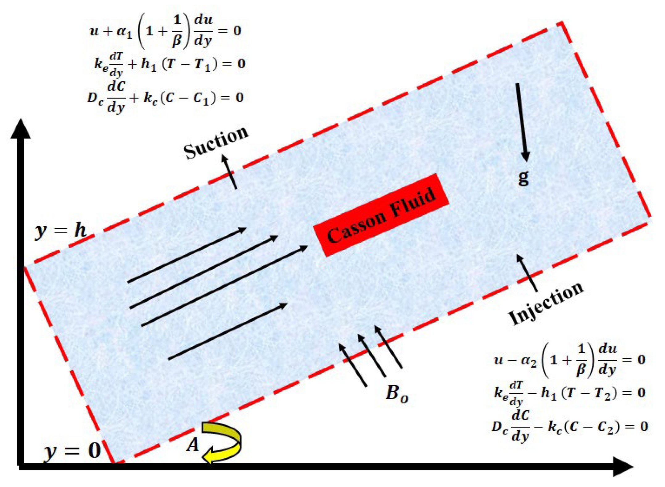
Figure 1: Fluid flow model.

The equation for continuity, momentum, energy, and concentration under the aforementioned assumptions and the linear Boussinesq’s approximation is as follows: Madhu et al. [20], Habibi-Matin & Pop [21], Hunt et al. [22]

The associate boundary conditions are:

At lower plate y = 0,

At upper plate y = h,

These boundary conditions describe a fluid confined between two parallel plates, with slip caused by non-Newtonian behavior or microscale factors. Heat is transferred between the plates and the fluid via conduction and convection. Mass transfer happens as a result of species diffusion and convective contact at the wall. Such conditions are frequently encountered in microfluidic devices, lubrication theory, polymer processing, and chemical reactors.

Introducing dimensionless variables:

Then

Subject to boundary conditions:

At η = 0 ,

At η = 1 , fη+β21+1βf′=0,θ′+BiTθη=0,φ′η+BiCφη=0(17) where Reynolds number, magnetic parameter, dimensionless pressure gradient, thermal Grashof number, solutal Grashof number, Prandtl number, Eckert number, thermo-diffusion/Soret parameter, thermal Biot number, solutal Biot number, Schmidt number, slip parameters at the lower and upper plates of the microchannels are defined below, respectively:

The following are the associated non-dimensional versions of the main physical parameters: skin friction coefficient, heat transfer rate (represented by the local Nusselt number), and Mass transfer rate (represented by the local Sherwood number).

5 Approximate Solution

The analytical solution of the coupled nonlinear differential Eqs. (13)–(15) with boundary conditions (16) and (17) is difficult and complex calculations. So, we have employed bvp4c solver (MATLAB) to obtain numerical solutions for given parametric values. The bvp4c is a finite difference code which executes three stages of Lobatto IIIa formula [23]. The bvp4c in MATLAB implemented step by step as follows:

Converting the problem into a system of first-order differential equations by introducing new variables.

• Assigning boundary conditions for the new variables;
• Guessing appropriate initial values for the new variable;
• Finally, calling inbuilt solver for solving first-order system.

For this we consider, f = ξ 1 , f ′ = ξ 2 , θ = ξ 3 , θ ′ = ξ 4 , φ = ξ 5 , φ ′ = ξ 6

Is the system of 1st order ODEs corresponding to the boundary conditions

6 Results and Discussion

In this section, we will present our numerical outcomes in the form of tables and figures. The validity of the numerical results is presented in Fig. 2. From this graph, it came to know that present results are fully matched with previously published results by setting β → ∞ , M = 0 , G r 1 = G r 2 = 0 , A = 0 , P = 1 and R e = 1 . Hence, this result indicates a good agreement with the reported values.

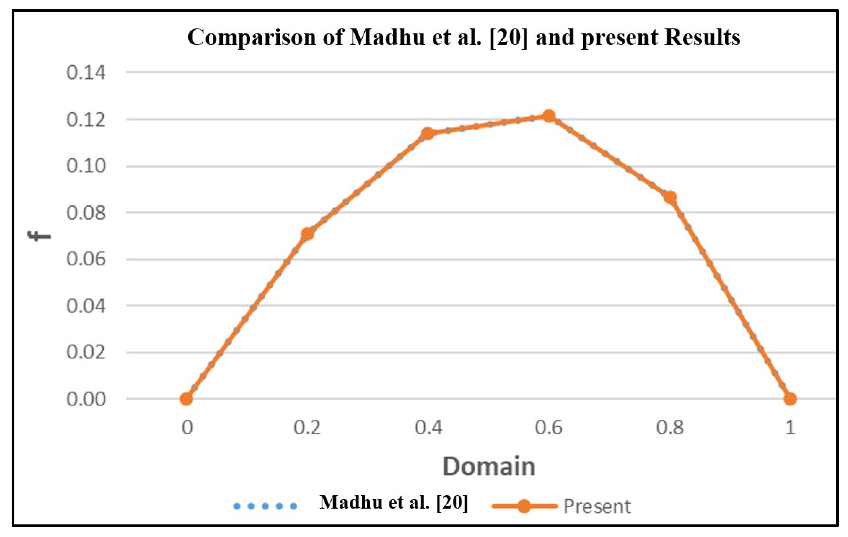
Figure 2: Validity of the numerical results [20].

Fig. 3a illustrates the trajectory of the dimensionless velocity f η in terms of the similarity variable η , with several values of the material fluid parameter β . An increase in β causes the velocity profile to move upwards, along with the maximum velocity going up. Fluids that contain a higher value of β denote non-Newtonian behavior and a faster movement of the fluid. The greater velocity is a consequence of a lower yield stress or greater deformation, allowing the fluid to flow more freely. When β gets large, fluid resistance declines, causing an increase in the flow. Fig. 3b shows how the flow control parameter A affects the fluctuation of the velocity profile f η based on the similarity variable. As A rises, velocity increases, particularly near the channel’s core. This means that the buoyant forces generated by the flow control parameter improve flow, most likely because heat gradients stimulate upward migration. The parabolic shape represents a fully developed laminar flow that is symmetrical about the channel’s centerline. This phenomenon has important uses in many technical fields, including chemical processing, solar energy systems, and electronic device cooling. Schematically, Fig. 3c depicts the influence of the dimensionless parameter, pressure gradient P , on the velocity f η . Peak velocity increases alongside P . This trend is to be expected because a larger pressure gradient increases fluid velocity by accelerating it. The profile remains parabolic, showing that inertia-induced effects are stronger near the channel center, while viscosity-induced effects are stronger near the walls. Pressure clearly helps to increase the fluid’s momentum, as seen by the fact that velocity increases as P rises. Fig. 3d shows the trend of slip parameter β 1 on the velocity profile f η at the lower plate. An increase in β 1 results in an increase in velocity close to the lower wall, indicating that slip causes a reduction in shear resistance. Increased wall velocity occurs when slide conditions undermine the no-slip boundary requirement. Increased slip allows for more fluid circulation over the surface, increasing the overall flow rate. The profile shows that the boundary layer continues to induce a decline in velocity towards the opposing wall. The velocity distribution at the upper wall for different values of slip parameter β 2 is shown in Fig. 3e. The velocity profile at the upper wall is directly proportional to β 2 . It is due to a decline in friction and an increase in flow due to the enhanced slip, which enables the fluid to move nearer the surface. The entire velocity profile is preserved to be parabolic, although the maximal velocity is slightly altered towards the centre. An increment in β 2 enhances improved flow at the upper bound. Fig. 3f demonstrates he variable of velocity against an increase in the magnetic parameter M . With an increase in M , the velocity decreases along the channel. This happens due to the Lorentz force arising out of the applied magnetic field, which resists the flow of the electrically conducting Casson fluid. The magnetic field damping effect has the effect of decreasing the momentum of the fluid, and this causes a thinner velocity boundary layer of the fluid. This is the behavior of magnetohydrodynamic (MHD) flow.

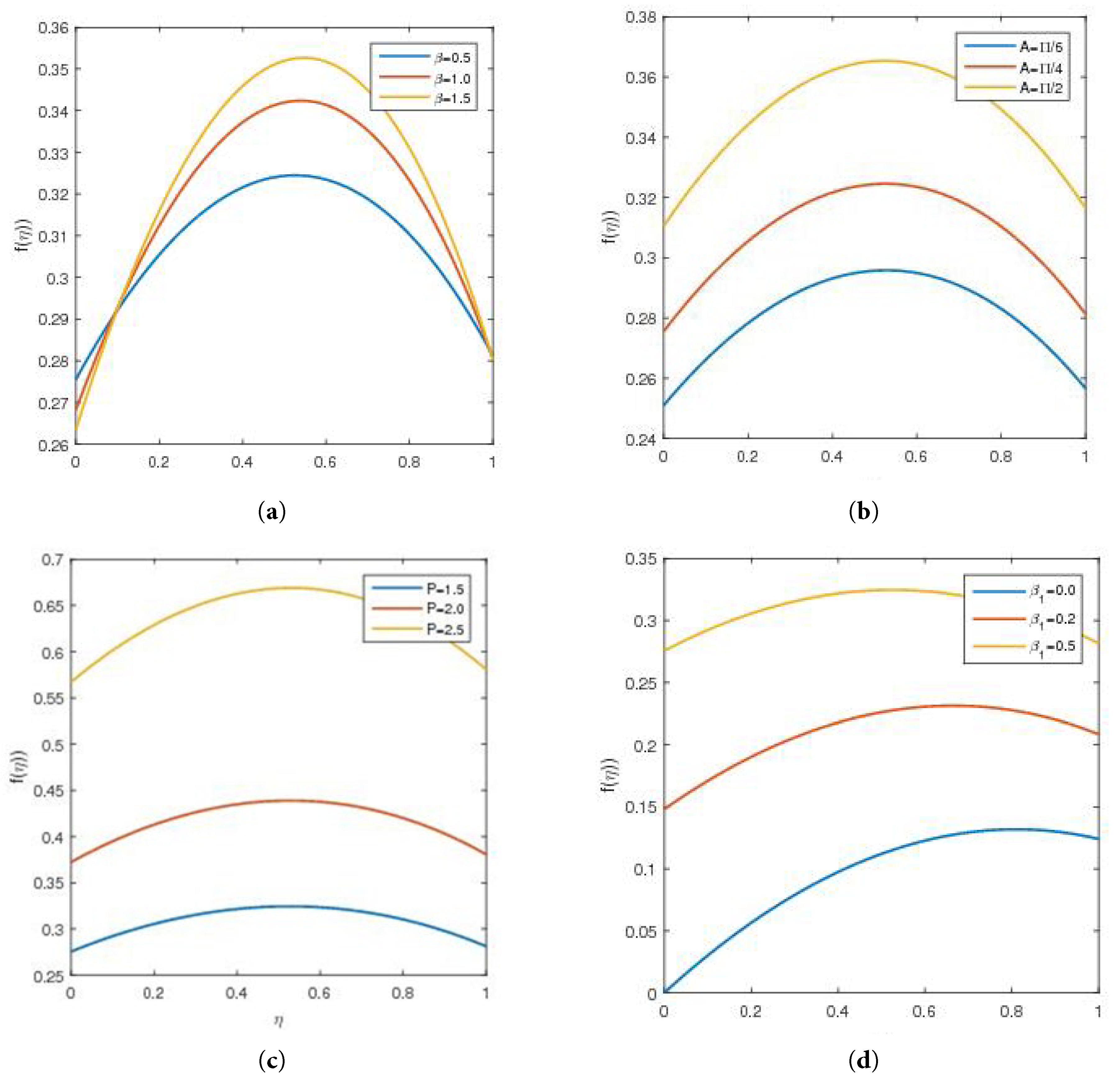
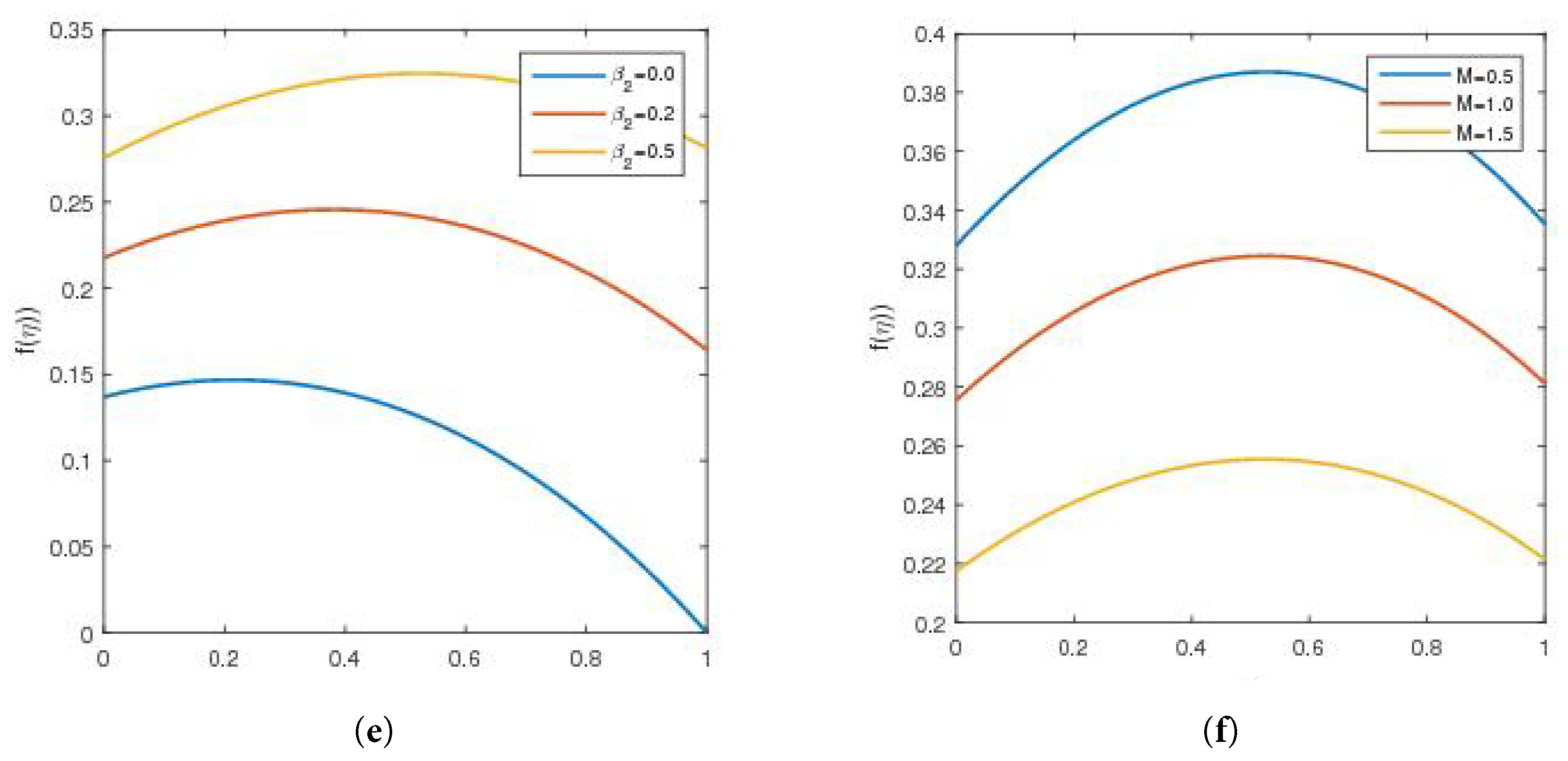
Figure 3: Effect of various physical parameters on velocity profile. (a) f η via β , (b) f η via A, (c) f η via P, (d) f η via β ₁, (e) f η via β ₂, (f) f η via M .

Fig. 4a illustrates the temperature profile θ(η) for various values of the material fluid parameter β. As β increases, the temperature rises throughout the channel, reflecting enhanced heat conduction due to non-Newtonian behavior, which promotes greater internal energy accumulation. The cooling from the hot wall to the cold wall follows the expected convection pattern in the boundary layer, with temperature decreasing along η. Fig. 4b shows the dimensionless temperature θ(η) at different values of the flow control parameter A. With increasing A, the temperature decreases more rapidly from the lower to the upper plate, especially near the heated wall. This occurs because larger values of A strengthen buoyancy forces, which accelerate fluid motion and enhance convective heat transfer. The intensified convective flow efficiently removes heat from the hot surface, leading to a shallower temperature gradient. The increasingly parabolic shape and steeper negative slope of the temperature profile with higher A indicate faster heat transport due to buoyancy-driven flow enhancement. This behavior is consistent with both forced and natural convection principles, which state that stronger fluid motion improves heat removal from heated surfaces. Fig. 4c demonstrates that the temperature decreases as the Biot number BiT increases. A higher Biot number indicates stronger surface convection relative to conduction, causing faster heat loss and a cooler boundary layer, consistent with classical heat-transfer theory. Finally, Fig. 4d shows that the temperature rises with an increase in the Eckert number Ec. Since Ec represents the ratio of kinetic energy to enthalpy, higher values correspond to stronger viscous dissipation, which elevates the fluid temperature.

This internal warmth negates any cooling, thus the temperature will be higher throughout the boundary layer on the larger E c values. With the increase of magnetic parameter M , the Lorentz force is generated by the magnetic field, thus suppressing the fluid velocity and decreasing convective heat transfer. As a consequence, less heat energy will be moved over the channel, hence reducing the overall temperature (see Fig. 4e). It is typical in MHD flows where velocity and heat transfer are diminished by the presence of magnetic damping. Fig. 4f suggests that there is a decrease in temperature with the increase in the pressure gradient P . A greater pressure gradient leads to an increased strength of flow that enhances convective heat transfer and increases the rate of heat removal by the hot wall. This results in a more pronounced decrease in temperature throughout the domain. Hence, the temperature profile θ η shows a decreasing trend with the increased pressure gradient P .

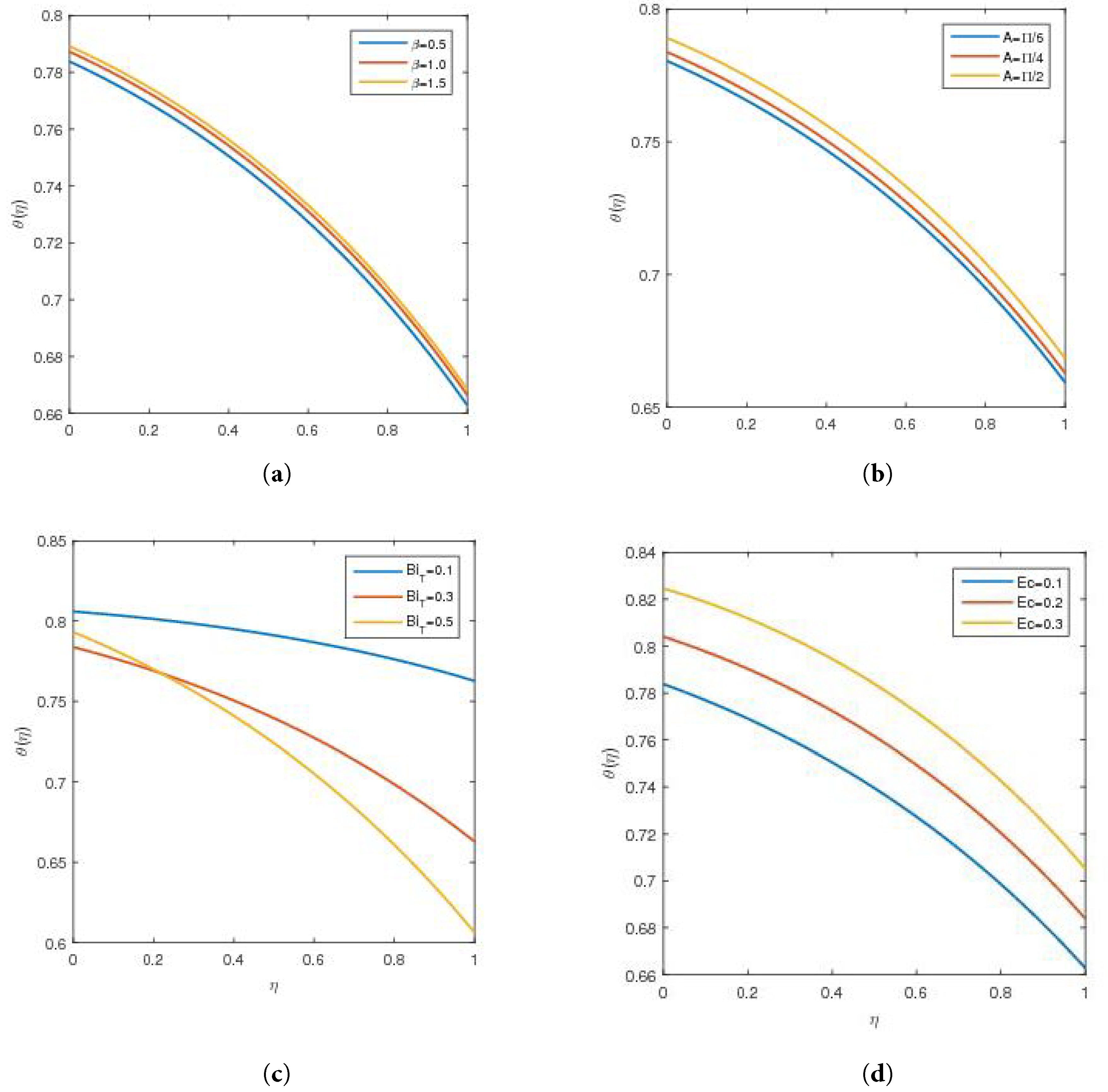
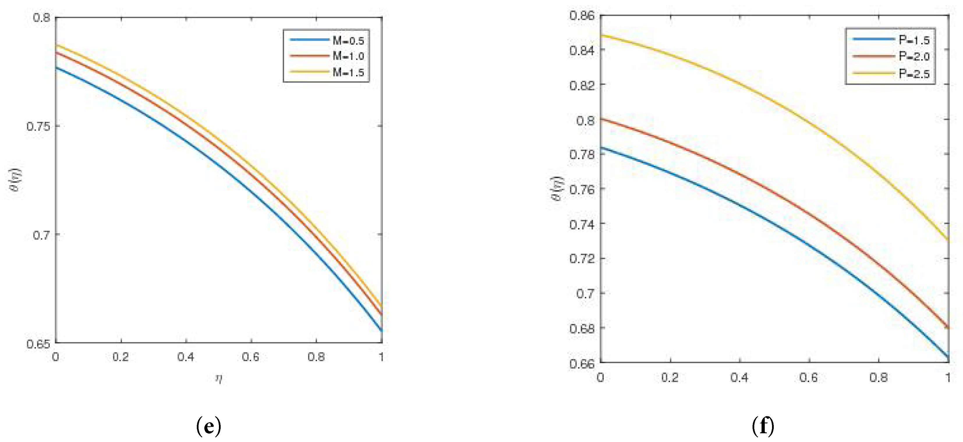
Figure 4: Effect of various parameters on temperature profile. (a) θ(η) vs. β, (b) θ(η) vs. A, (c) θ(η) vs. Bi_T, (d) θ(η) vs. E_c, (e) θ(η) vs. M, (f) a) θ(η) vs. P.

Fig. 5 represents the concentration profile along with the parameters solutal Biot number B i C , thermal Biot number B i T , Eckert number E c , pressure gradient P , Schmidt number ( S C ) , and thermo-diffusion/Soret parameter ( S r ) . The variation of concentration ϕ η with the solutal Biot number B i C is given in Fig. 5a. The concentration gradient gets steeper with the increase in the height of B i C , meaning that there will be an increase in the transfer of mass between the surface to the fluid. Higher B i C represents an improvement of mass diffusion in the boundary layer, leading to a more adverse increase in the solute concentration when we move away from the wall. B i t is most usually associated with the transmission of heat, yet indirectly it also has an impact on mass transport. Fig. 5b illustrates that the higher the B i t , the steeper the concentration profiles. This is attributed to heightened convective flows that have been brought about by heat phenomena, which change solute dispersion. More rapid convection of heat enables mass to be removed better in the near-wall zone. The concentration profile ϕ η shows a downward trend more rapidly when the Eckert number increases (shown in Fig. 5c). An increase in viscous dissipation promotes thermal energy, enhances convective mixing, and reduces solute concentration along the wall. Such anti-correlation brings relevance to the interconnection of heat and mass transport systems, where the effect of dissipation is serious. Effects of pressure gradient P on the concentration profile ϕ η are displayed in Fig. 5d. The concentration decreases rapidly with the increase in the pressure gradient. The augmented velocity due to the pressure gradient leads to a greater convective solute transport, which reduces the solute concentration at the wall. The trend is observed at the simultaneous higher flow rates that lead to faster solute dispersion. Schmidt number is the ratio of the momentum diffusivity to the diffusivity of mass. The larger the S c , the smaller the diffusivity of mass, the higher the concentration gradients. Fig. 5e gives the concentration profile along with the Schmidt number. With the increased concentrations of S c , concentration drops due to the fact that the growing tendency is associated with the solute remaining near the wall and limited diffusion to the bulk fluid. Lastly, Fig. 5f represents the influences of the thermos-diffusion/Soret parameter S r on the concentration ϕ η . Soret effect, as a reaction to the temperature gradients, causes the migration of the solutes. An increment in S r results in a faster fall in concentration over the domain. Also, the increased thermal diffusion causes a higher concentration gradient, withdrawing the solutes far away from the heated wall. This property is very important in systems where there is Heat and Mass Transfer.

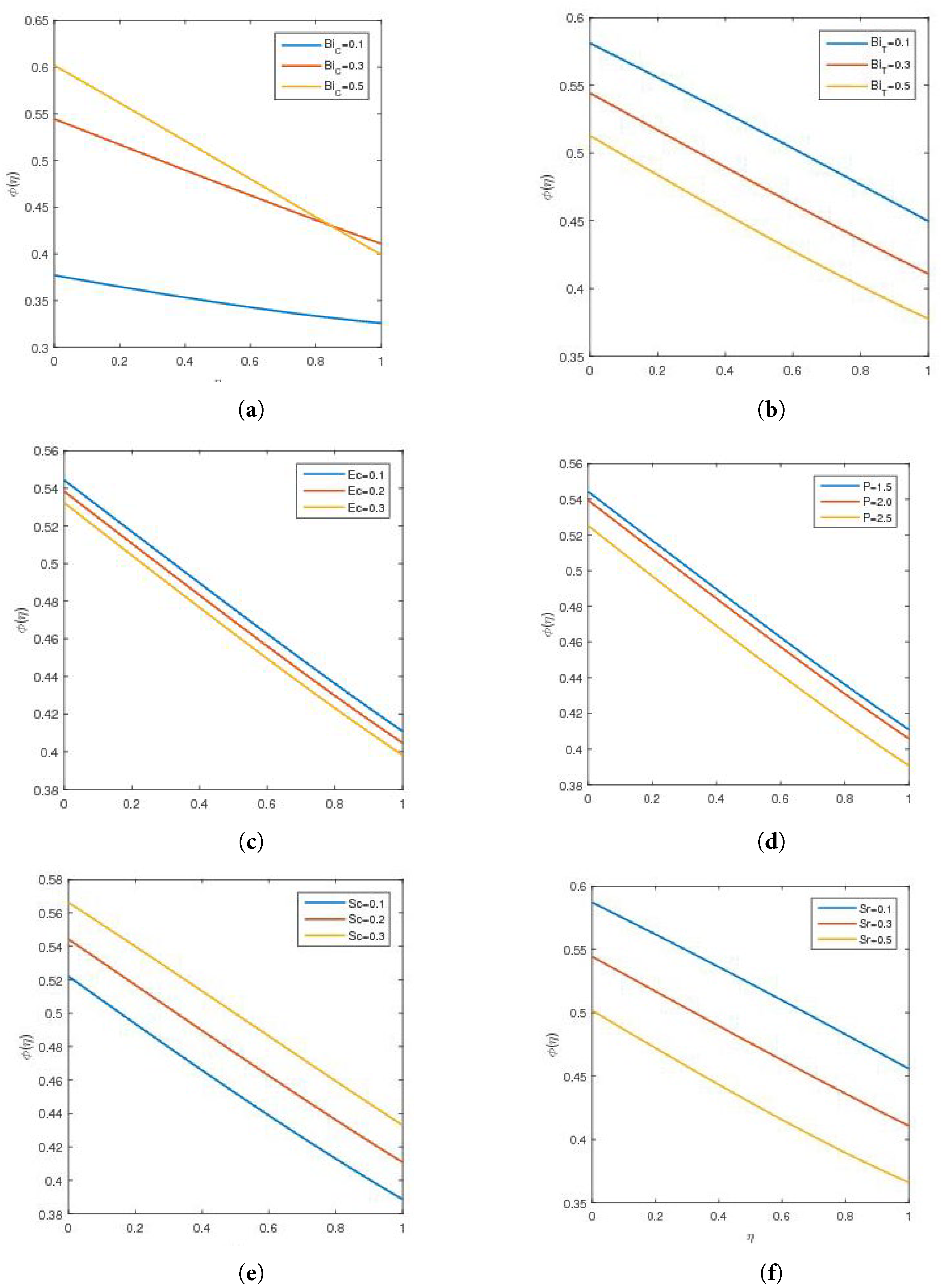
Figure 5: Effect of various parameters on concentration profile. (a) ϕ (η) vs. Bi_C, (b) ϕ (η) vs. Bi_T, (c) ϕ (η) vs. Ec, (d) ϕ (η) vs. P, (e) ϕ (η) vs. Sc, (f) ϕ (η) vs. Sr.

6.1 Taguchi-Grey Relational Analysis (GRA)-Principal Component Analysis (PCA)

Principal Component Analysis (PCA), together with Taguchi-Grey Relational Analysis (GRA), serves as two multi-objective optimization techniques that are adopted: Taguchi’s Sturdy Design for noise reduction and experimental design. The method of Grey Relational Analysis (GRA) generates one unified performance index when analyzing multiple answers. PCA simplifies weighting through principal component analysis while stopping subjective bias from occurring. Engineers widely employ this method to optimize processes that have conflicting goals in their work related to manufacturing and quality improvement, and engineering.

Taguchi Experimental Design (Orthogonal Arrays)

Taguchi achieves statistical effectiveness through Orthogonal Arrays (OA), which reduce experimental requirements. We are using L27 (35), which means 27 experiments with 5 factors, each at 3 levels. We have three cases, the first case is of skin friction for which we have responses at C f x 0 and C f x 1 . The factor we are dealing with in the case of skin friction, Beta (Casson parameter), G r 1 (Thermal Grashof number), G r 2 (Solutal Grashof number), β 1 (slip parameter at lower wall), and β 2 (slip parameter at upper wall). The experimental layout for skin friction case is given in Table 1.

The next case of Nusselt number, N u x 0 at the lower wall and N u x 1 at the upper wall. The factors involved are Beta (Casson parameter), R e (Reynolds number), E c (Eckert number), M (Magnetic parameter), and B i T (Thermal Biot number) shown in Table 2.

The third and the last case is of Sherwood number, and we have the responses at the lower wall S h x 0 as well as at the upper wall S h x 1 . The parameters involved in this case are S r (thermo-diffusion/Soret parameter), S c (Schmidt number), R e (Reynolds number), B i c (Solutal Biot number), and β (Casson parameter). The experimental layout is L27 (design matrix), given in Table 3.

The first step of optimization is to calculate the S / N ratio for the responses using the following formulas. For the lower, the better:

The higher, the better: SN=−10log101n∑m=1Z1Zim2(22) here, i = 1 , … , y , m = 1 , … , Z , Z represents the number of observed responses, n is the number of variations in responses, and i represents the experiments. And the formula for nominal the best is: SN=10log10μ2σ2(23) μ is the mean of the responses, and σ 2 is the standard deviation. Process parameter optimization through S / N ratio analysis allows researchers to select ideal settings that improve product quality, together with consistency, along with reduced defect rates. The S/N ratio represents a data-focused plan that enhances system reliability while maintaining operational efficiency, thus becoming essential for industrial quality engineering and optimization applications.

A higher S / N ratio indicates it is closer to the target and has less variance.

6.2 Grey Relational Analysis

The optimization method (GRA) merges multiple answers into one outcome. The Grey Relational Analysis (GRA) technique operates on complex systems that use imprecise and ambiguous, and partial data to evaluate and optimize response factors. The method resolves multi-response optimization problems across engineering sectors as well as management and quality control fields. GRA depends on the concept of grey systems, which describes insufficient or nonexistent information levels. Through GRA, researchers can identify relationships between response variables and factors, which subsequently allows them to establish priorities based on influence and similarity. GRA determines experimental data relationships with reference values through the gray relational coefficient (GRC) process. GRA functions ideally whenever diverse criteria and responses must be optimized at once. The different units and scales of responses in evaluation lead to the implementation of normalization processes. Table 4, given below, gives the numerically calculated data of Skin Friction. For the detailed calculations.

In our study, we are treating C f x as lower the better, and both N u x and S h x as higher the better. We have used the following formulas for normalization: Xim=maxZim−ZimmaxZim−minZimfor lower the better(24) and, Xim=Zim−minZimmaxZim−minZimfor highr the better(25)

In the above two equations, X i m is the normalized value for the corresponding responses, Z i m represents the original observed response values, min Z i m is the minimum, and max Z i m is the maximum observed response value. The next step is to calculate the deviation sequence. It is an important step in GRA because it tells how far the data is from the ideal situation. The ideal situation that is used to measure the difference is 1. The smaller values mean the response is closer to the ideal situation, hence better performance, and vice versa. So, the formula for the deviation sequence is represented and given as: Δim=Xm−Xim(26) X m is the ideal case, which is 1, and X i m is the normalized data calculated in the previous step. In the GRA, the next step is to calculate the Grey Relational Coefficient (GRC), which measures the similarity between the observed data and the ideal situation. The degree of measured response matching the optimal value in Grey Relational Analysis (GRA) is measured through Grey Relational Coefficient (GRC), which produces values between 0 and 1. The GRC can be calculated using the equation below: Ωim=Δmin+ΨΔmaxΔim+ΨΔmax(27) Ψ , named as a distinguishing coefficient, can be anywhere from 0–1. Here, in our case, we have taken it as 0.5 ([19]) which is a common practice.

Table 5 represents the S/N ratio, normalized data, deviation sequence, and the GRC values for Table 2.

Table 6 gives us the numerical values of S/N ratio, normalized data, deviation sequence, and the GRC values, calculated by using Eqs. (22), (25)–(27). The next step is to find the Grey Relational Grade (GRG), which is the average of all the corresponding GRC values. Eq. (28), given below, represents the GRG.

The Grey Relational Grade (GRG) serves as a single performance score (0–1) that ranks experimental runs in multi-objective optimization. The system generates one comprehensive performance measure from multiple conflicting analysis results. The situation delivers the lowest performance results when GRG reaches 0 and maximum performance results when GRG is 1 . Hence, we can rank the experiments based on the GRG values and the optimal/best experiment setting.

6.3 Principal Component Analysis

Before PCA execution, we determine the mean value of all dataset columns or responses. The procedure centers data before running PCA because this method is sensitive to data alignment. The mean vector represents the central point of the data within the domain. We will find the mean of the GRC columns, and the formula to find the mean is given as Eq. (29).

In the above equation, μ is the mean of the GRC for each response, and Ω i m is the GRC column. PCA operates by finding directions (principal components) that represent high data fluctuation. A centered dataset enables the first principal component to locate the direction of maximum variance, but it will show a mean vector orientation when the data points are not centered. The formula for centering the data is denoted and written as:

Centered data allows the principal components to stay unaffected by systematic offsets so they can directly track the maximum variation directions within the data.

The process of data centering requires subtraction of the mean from each data point. Covariance calculations achieve significance because the data maintains an even distribution around zero. The next step is to calculate the covariance matrix. The covariance matrix shows how all the responses change with each other. Covariance helps in understanding relationships between responses, at the same time, PCA identifies the main directions of data variation. The relationship between two variables becomes interdependent when their absolute covariance value is high, but exists as independent variables when this value reaches zero. The covariance matrix can be calculated by the following formula, involving the variance of G 1 1 , the variance of G 1 2 and the covariance of G 1 1 and G 1 2 ; N=varG11covG11,G12covG11,G12varG12(31) where, varG11=1Z−1∑m=1ZG11m−μG112(32) varG21=1Z−1∑m=1ZG21m−μG212(33) and,

In Eqs. (31)–(34), Z is the number of experiments, v a r G 1 1 is the variance of the G 1 1 , G 1 2 represents the variance of G 1 2 , c o v G 1 2 , G 1 2 is the covariance of G 1 1 and G 1 2 , and μ is the mean.

The next step after calculating the covariance matrix is to calculate the eigenvalues using Eq. (35) detC−λI=0(35) C the covariance matrix here facilitates the finding of Principal components, while I represents the identity matrix. Solving Eq. (35) for λ gave us the eigenvalues see in Table 7. Now, for each value of λ , we can find the eigenvectors by the following equation,

The total variance can be calculated by adding both the eigenvalues as follows:

Now, the contribution of each principal component (PC) can be calculated by using the following formula: Contribution of PC1=λ1λ×100(38) and,

We can see the individual contributions of PC’s in Table 7. We can see that the contribution of the PC1 is far greater than the PC2. PC1 in all three cases, explains most of the total variance, making it the most important PC while the lesser contribution of PC2 means it is adding additional information but contributing less than PC1. So we have ignored PC2 and used PC1 only while calculating the GRG(P) which is the Grey Relational Grade by Principal Component Analysis.

The way to generate GRG(P) begins with a calculation using weights from PC1. Our first step turned the square of α and β into a linear combination with GRC to determine GRG(P) with the aid of data in Table 7. Our investigation needs the following two Eqs. (40) and (41), for GRG(P) calculation.

The primary focus is on PC1, as it accounts for the largest proportion of variance in the analysis. Table 8 presents a comparison of experimental rankings obtained from Grey Relational Analysis (GRA) and Principal Component Analysis (PCA) for skin friction. Both methods identify Experiment 9 as the highest-ranked case, confirming consistency between the two approaches. Similarly, Table 9 and Table 10 demonstrate that the same experiments are identified as optimal when using either GRA or PCA. Specifically, Table 9 highlights Experiment 3, while Table 10 identifies Experiment 12 as the best-performing case (emphasized in bold and underlined). These results validate the reliability and accuracy of our optimization methodology.

7 Conclusion

This study presents a comprehensive numerical and optimization analysis of MHD thermosolutal convection for a Casson fluid within an inclined, permeable microchannel featuring convective boundary conditions. The governing nonlinear equations were solved using MATLAB’s bvp4c solver, while a hybrid Taguchi–Grey Relational Analysis (GRA) and Principal Component Analysis (PCA) framework was employed to perform a systematic, design-oriented evaluation of heat and mass transfer performance. The results show strong agreement with prior studies, validating both the modeling approach and the incorporation of non-Newtonian behavior under magnetic field effects.

Key findings include:

• (i)Velocity-slip and solutal effects significantly impact flow and concentration fields, while thermal impacts affect temperature distribution
• (ii)PC1 captures the dominant portion of system variability, justifying its use as the principal driver in the GRG-PCA optimization; and
• (iii)The integrated GRA–PCA methodology reliably identifies optimal operating scenarios, with GRA and PCA yielding consistent rankings across skin friction, Nusselt, and Sherwood responses.

Overall, the methodology offers actionable guidance for the design and control of microfluidic systems employing Casson fluids under electromagnetic effects, with potential extensions to broader non-Newtonian, multicomponent flows.

References

1. Verma AK . Numerical investigation of unsteady magnetohydrodynamic flow of a Newtonian fluid with variable viscosity in an inclined channel. Phys Fluids. 2025; 37: 013623. doi:10.1063/5.0248969. [Google Scholar] [CrossRef]
2. Das UJ , Majumdar NM . An analytical approach to magnetohydrodynamic flow on an inclined channel with induced magnetic field and heat radiation. Lat Am Appl Res Int J. 2024; 54( 3): 313– 8. doi:10.52292/j.laar.2024.3109. [Google Scholar] [CrossRef]
3. Mani R , Krishna GG . Entropy analysis of MHD flow of Jeffrey fluid in an inclined channel. Heat Transf. 2022; 51( 6): 5789– 807. doi:10.1002/htj.22569. [Google Scholar] [CrossRef]
4. Sharma RP , Ghosh SK , Das S . MHD flow in a rotating channel surrounded in a porous medium with an inclined magnetic field. In: Energy systems and nanotechnology. Singapore: Springer; 2021. p. 369– 84. doi:10.1007/978-981-16-1256-5_18. [Google Scholar] [CrossRef]
5. Kumar S , Vishwanath S . Hall and ion-slip effects on MHD free convective flow of a viscoelastic fluid through porous regime in an inclined channel with moving magnetic field. Kragujevac J Sci. 2020( 42): 5– 18. doi:10.5937/KgJSci2042005K. [Google Scholar] [CrossRef]
6. Riaz S , Ali S , Ali Q , Khan SU , Amir M . Fractional simulations for mixed convection flow of hybrid nanofluids due to inclined channel with chemical reaction and external heat source features. Waves Random Complex Medium. 2013: 1– 19. doi:10.1080/17455030.2023.2226749. [Google Scholar] [CrossRef]
7. Bala Anasuya J , Srinivas S . Heat transfer characteristics of magnetohydrodynamic two fluid oscillatory flow in an inclined channel with saturated porous medium. Proc Inst Mech Eng Part E J Process Mech Eng. 2024; 238( 1): 427– 40. doi:10.1177/09544089221146364. [Google Scholar] [CrossRef]
8. Elmhedy Y , Abd-Alla AM , Abo-Dahab SM , Alharbi FM , Abdelhafez MA . Influence of inclined magnetic field and heat transfer on the peristaltic flow of Rabinowitsch fluid model in an inclined channel. Sci Rep. 2024; 14( 1): 4735. doi:10.1038/s41598-024-54396-z. [Google Scholar] [CrossRef]
9. Boujelbene M , Rehman S , Alqahtani S , Alshehery S , Eldin SM . Thermal transport and magnetohydrodynamics flow of generalized Newtonian nanofluid with inherent irreversibility between conduit with slip at the walls. Eng Appl Comput Fluid Mech. 2023; 17( 1): 2182364. doi:10.1080/19942060.2023.2182364. [Google Scholar] [CrossRef]
10. Sri Ramachandra Murty P , Balaji Prakash G , Karuna Sree C . Rotating hydromagnetic two-fluid convective flow and temperature distribution in an inclined channel. Int J Eng Technol. 2018; 7( 4.10): 629– 35. doi:10.14419/ijet.v7i4.10.21298. [Google Scholar] [CrossRef]
11. Naseem T , Mebarek-Oudina F , Vaidya H , Bibi N , Ramesh K , Khan SU . Numerical analysis of entropy generation in joule heated radiative viscous fluid flow over a permeable radially stretching disk. Comput Model Eng Sci. 2025; 143( 1): 351– 71. doi:10.32604/cmes.2025.063196. [Google Scholar] [CrossRef]
12. Alshareef TS . The effect of Wall’S porous liner on MHD couette flow of carreau fluid in an inclined channel under the convective conditions. Int J Heat Technol. 2024; 42( 1): 61– 70. doi:10.18280/ijht.420107. [Google Scholar] [CrossRef]
13. Mebarek-Oudina F , Dharmaiah G , Rama Prasad JL , Vaidya H , Kumari MA . Thermal and flow dynamics of magnetohydrodynamic Burgers’ fluid induced by a stretching cylinder with internal heat generation and absorption. Int J Thermofluids. 2025; 25: 100986. [Google Scholar]
14. Kumar MA , Mebarek-Oudina F , Mangathai P , Shah NA , Vijayabhaskar C , Venkatesh N , et al. The impact of Soret Dufour and radiation on the laminar flow of a rotating liquid past a porous plate via chemical reaction. Mod Phys Lett B. 2025; 39( 10): 2450458. doi:10.1142/s021798492450458x. [Google Scholar] [CrossRef]
15. Mebarek-Oudina F , Bouselsal M , Djebali R , Vaidya H , Biswas N , Ramesh K . Thermal performance of MgO-SWCNT/water hybrid nanofluids in a zigzag walled cavity with differently shaped obstacles. Mod Phys Lett B. 2025; 39( 29): 2550163. doi:10.1142/s0217984925501635. [Google Scholar] [CrossRef]
16. Vinutha K , Madhukesh JK , Patil N , Abdulrahman A . Numerical analysis of heat and mass transfer in off-centered stagnation point Casson fluid flow over a rotating disc with thermophoretic particle deposition and artificial neural network-based optimization. Eng Appl Artif Intell. 2025; 160: 112041. [Google Scholar]
17. Vinutha K , Madhukesh JK , Prasad KV , Kulshreshta A , Ali Shah N , Yar M . MHD Casson nanofluid flow over a three-dimensional exponentially stretching surface with waste discharge concentration: a revised Buongiorno’s model. Appl Rheol. 2025; 35: 20250040. doi:10.1515/arh-2025-0040. [Google Scholar] [CrossRef]
18. Manohar GR , Venkatesh P , Gireesha BJ , Ramesh GK . Numerical treatment for Casson liquid flow in a microchannel due to porous medium: a hybrid nanoparticles aspects. Proc Inst Mech Eng Part C J Mech Eng Sci. 2022; 236( 2): 1293– 303. doi:10.1177/09544062211008933. [Google Scholar] [CrossRef]
19. Raza J , Mebarek-Oudina F , Ali H , Sarris IE . Slip effects on casson nanofluid over a stretching sheet with activation energy: RSM analysis. Front Heat Mass Transf. 2024; 22( 4): 1017– 41. doi:10.32604/fhmt.2024.052749. [Google Scholar] [CrossRef]
20. Madhu M , Shashikumar NS , Gireesha BJ , Kishan N . Second law analysis of Powell–Eyring fluid flow through an inclined microchannel with thermal radiation. Phys Scr. 2019; 94( 12): 125205. doi:10.1088/1402-4896/ab32b7. [Google Scholar] [CrossRef]
21. Matin MH , Pop I . Forced convection heat and mass transfer flow of a nanofluid through a porous channel with a first order chemical reaction on the wall. Int Commun Heat Mass Transf. 2013; 46: 134– 41. [Google Scholar]
22. Hunt G , Karimi N , Torabi M . Two-dimensional analytical investigation of coupled heat and mass transfer and entropy generation in a porous, catalytic microreactor. Int J Heat Mass Transf. 2018; 119: 372– 91. [Google Scholar]
23. Reza J , Mebarek-Oudina F , Makinde OD . MHD slip flow of Cu-kerosene nanofluid in a channel with stretching walls using 3-stage lobatto IIIA formula. Defect Diffus Forum. 2018; 387: 51– 62. [Google Scholar]
Cite This Article
Copyright © 2025 The Author(s). Published by Tech Science Press.
This work is licensed under a Creative Commons Attribution 4.0 International License , which permits unrestricted use, distribution, and reproduction in any medium, provided the original work is properly cited.
Downloads
Citation Tools