
 Submit a Paper
 Propose a Special lssue
 Open Access
ARTICLE

Analysis of Fluid Flow and Optimization of Tubing Depth in Deep Shale Gas Wells
School of Petroleum Engineering, Yangtze University, Wuhan, 430100, China
* Corresponding Author: Jie Liu. Email:
Fluid Dynamics & Materials Processing 2025, 21(3), 529-542. https://doi.org/10.32604/fdmp.2024.057535
Received 20 August 2024; Accepted 28 November 2024; Issue published 01 April 2025
 View Full Text
 Download PDF
Abstract
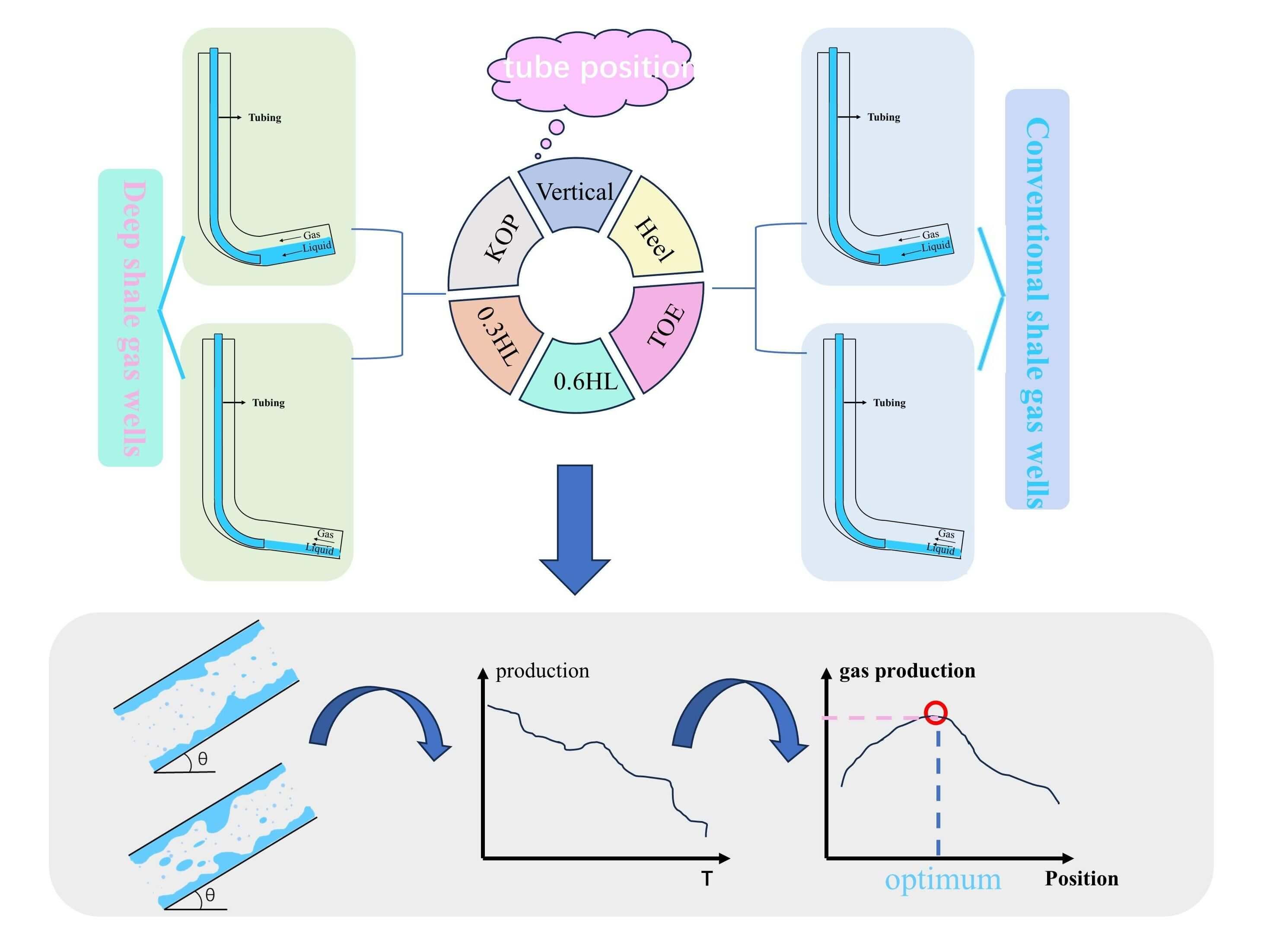
As shale gas technology has advanced, the horizontal well fracturing model has seen widespread use, leading to substantial improvements in industrial gas output from shale gas wells. Nevertheless, a swift decline in the productivity of individual wells remains a challenge that must be addressed throughout the development process. In this study, gas wells with two different wellbore trajectory structures are considered, and the OLGA software is exploited to perform transient calculations on various tubing depth models. The results can be articulated as follows. In terms of flow patterns: for the deep well A1 (upward-buckled), slug flow occurs in the Kick-off Point position and above; for the deep well B1 (downward-inclined), slug flow only occurs in the horizontal section. Wells with downward-inclined horizontal sections are more prone to liquid accumulation issues. In terms of comparison to conventional wells, it is shown that deep shale gas wells have longer normal production durations and experience liquid accumulation later than conventional wells. With regard to optimal tubing placement: for well A1 (upward-buckled), it is recommended to place tubing at the Kick-off Point position; for well B1 (downward-inclined), it is recommended to place tubing at the lower heel of the horizontal section. Finally, in terms of production performance: well A1 (upward-buckled) outperforms well B1 (downward-inclined) in terms of production and fluid accumulation. In particular, the deep well A1 is 1.94 times more productive and 1.3 times longer to produce than conventional wells. Deep well B1 is 1.87 times more productive and 1.34 times longer than conventional wells.Graphic Abstract
Keywords
With the development of shale gas, the horizontal well fracturing production model has been widely adopted [1], significantly enhancing the industrial gas flow of shale gas wells. However, the rapid decline in single-well production is a reality that must be faced during the development process [2,3]. The gas well loading phenomenon is considered one of the most serious problems in the gas industry. It occurs as a result of liquid accumulation in the wellbore when the gas phase does not provide sufficient energy to lift the produced fluids, imposing additional hydrostatic pressure on the reservoir and causing more reduction in the transport energy [4]. Therefore, it is necessary to take measures to extend the production time of gas wells, and the current measures for draining gas recovery at home and abroad mainly include Depletion Compression (DC), Automated Intermittent Production (AIP) [5], Velocity tube columns (VS) [6], Downhole Check Valve (DCV) [7], Plunger Lift (PL) [8], Foam Assisted Lifting (FAL) [9], Artificial Gas Lift (AGL) [10] and Downhole Pumps (DP) [11]. The most commonly used measures for the drainage and recovery process include installing smaller inserted tubing columns in the original tubing to reduce the completion ID and thus Qmin.
Current study on these two aspects usually involves three main approaches: physical simulation, numerical calculation, and numerical simulation. The physical simulation is a research method guided by indoor experiments on two-phase gas-liquid flow, numerical calculation is a research method based on the minimum pressure drop theory, evaluated using multiphase pipe flow pressure drop formulas [12,13], and numerical simulation is a research method that employs commercial software to simulate the flow of fluids within the wellbore. Beggs and Brill experimentally investigated the relationship between cross-section liquid holding capacity and pipe drag coefficient and firstly proposed a pressure drop calculation model for inclined two-phase pipe flow [14]. Hewitt et al. classified the flow patterns into bubble flow, segment plug flow, stirred flow, annular flow and ring fog flow by the experimental data of two-phase flow of air-water and steam-water [15]. Asghar et al. performed a numerical simulation of a two-phase flow pressure drop and verified several two-phase flow pressure drop calculation models [16]. Deendarlianto et al. [17] performed numerical simulation of two-phase flow in a horizontal pipe and corrected the flow pattern diagram of Mandhane et al. [18]. Yang et al. [19] conducted a systematic analysis of flow patterns under different pipe diameters, inclinations, and flow types for gas-liquid production conditions in a certain gas field through laboratory simulations. They employed flow pattern identification methods, liquid holdup calculation methods, and pressure drop calculation methods. Using experimental data, they evaluated different flow pattern classification methods. By introducing the Reynolds number, they proposed a new pressure drop calculation model. Salim et al. developed a critical gas velocity model based on experimental results to determine the minimum amount of gas required for gas to carry liquids by means of transients [20]. Zhang numerical simulation of the phenomenon of gas-liquid two-phase flow in a round pipe with different inclination angles as well as in production casing, combined with experiments, and verified several mathematical models of two-phase flow [21]. Pang used numerical simulation to study the gas-liquid two-phase flow of deep coalbed methane wells under high pressure, and got the rule of change of the parameters of gas-liquid two-phase flow by the study of its flow pattern and pressure drop [22]. The previous research is mainly in the modified empirical formulas obtained through experimental results and numerical simulation under specific working conditions. In view of the fact that the fluid accumulation problem in deep shale gas wells is relatively less studied at present, in order to study the production of deep shale gas wells under different tubing depths, this paper adopts transient numerical simulation to study the gas-liquid flow law in the whole wellbore of deep shale gas wells, to explore the reasonable tubing lowering position, and will discuss the differences with conventional shale gas wells.
2 Dynamic Modelling of Gas Well Production
In order to clarify the flow pattern of wellbore fluids in deep shale gas wells, the Well Liquid Loading module of OLGA software was selected for the simulation. Initially, the PVTsim software is employed to generate the tabular component file for natural gas, utilizing the SRK equation of state for real gases. Subsequently, the enhanced two-fluid model is selected as the mathematical framework for the simulation computations. A physical model of the shale gas horizontal wells is then developed, leveraging data from two distinct well trajectories originating from the same drilling platform. In the final stage, the simulation’s boundary and initial conditions are established based on the actual production data from the Weiyuan shale gas field.
Multiphase flow models encompass a variety of approaches, such as flow pattern models, homogeneous flow models, split-phase flow models, drift flow models, and two-fluid models, among others. Notably, two-fluid models, which are grounded in conservation equations, offer a versatile solution for different types of flow phenomena. In this study, an extended two-fluid model is employed, which includes the gas phase, the liquid film phase, and the liquid droplets that are entrained within the gas phase. This model is utilized to capture the complexities of multiphase flow in a comprehensive manner.
Horizontal wells A1 and B1 with different well trajectories on the same platform in the shale gas field are selected, and two different well structures, horizontal section upturned and horizontal section downturned, are constructed based on their logging data, as shown in Fig. 1. In order to facilitate the comparative analysis of the fluid accumulation pattern of deep and conventional shale gas wells, the well trajectory of deep shale gas wells is constructed by reducing the vertical section by 1000 m to construct the well structure of the conventional shale gas horizontal wells, in which A and B are the conventional shale gas wells with upward and downward curvature of the horizontal section, respectively.
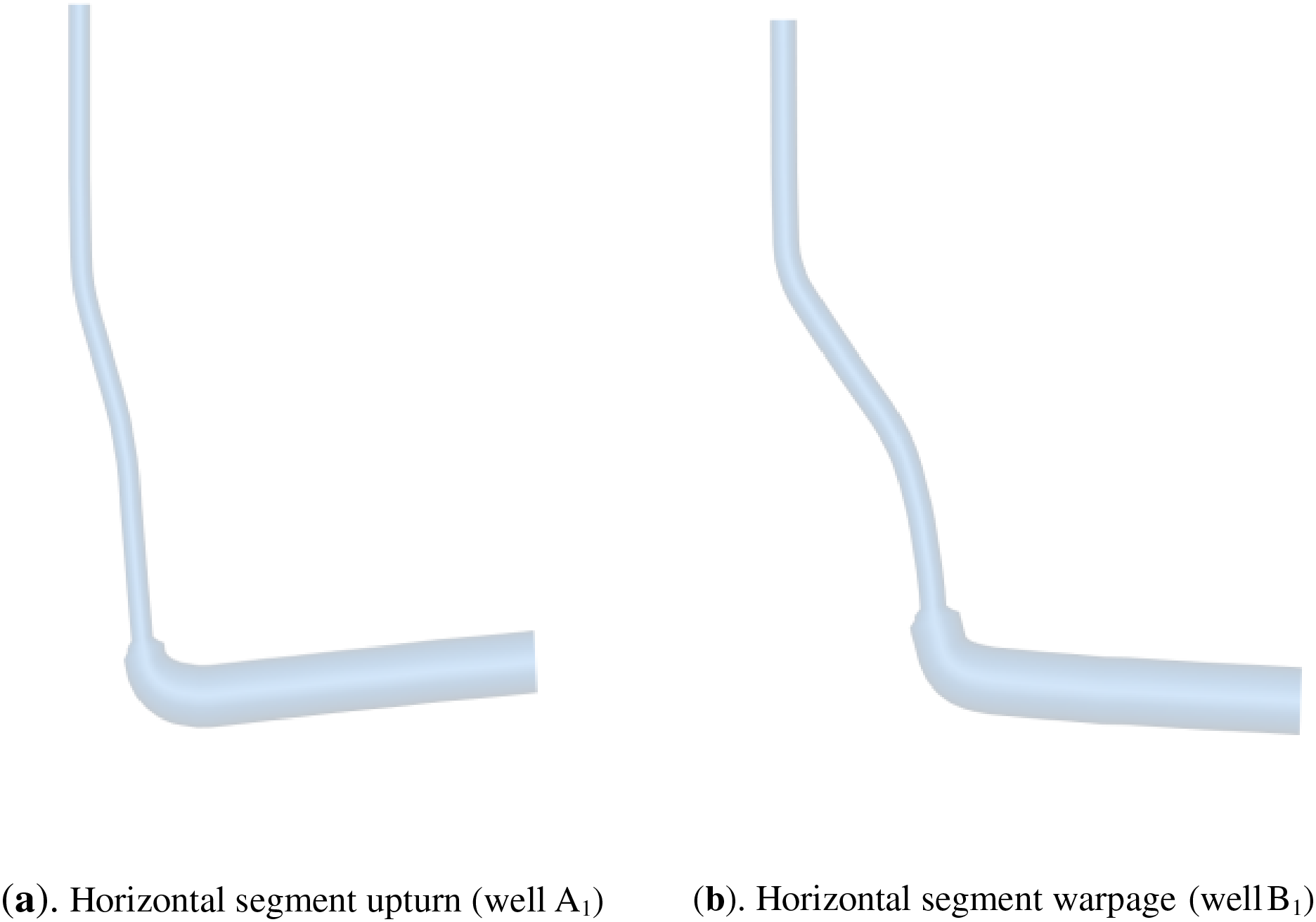
Figure 1: Schematic diagram of well structure of wells A1 and B1
In order to study the flow patterns of gas and liquid in the wellbore at different depths of the tubing, physical models were established for six different tubing depths in the constructed wellbore: vertical section, Kick-off Point (KOP), horizontal section heel, Horizontal segment at 1/3 (1/3HL), Horizontal segment at 2/3 (2/3HL), and toe of horizontal section (TOE). Simulated gas-liquid flow in a gas well when the water-gas ratio is 0.000775.
2.2.3 Production Capacity Equation
Whether the horizontal section is upturned or downturned, the same gas well production Eq. (1) is selected for numerical simulation in order to facilitate the comparative analysis of the fluid accumulation pattern [23].
where PR is the average formation pressure, Pwf is the average bottom-hole flowing pressure, and qg is the daily gas production rate.
2.2.4 Boundary and Initial Conditions
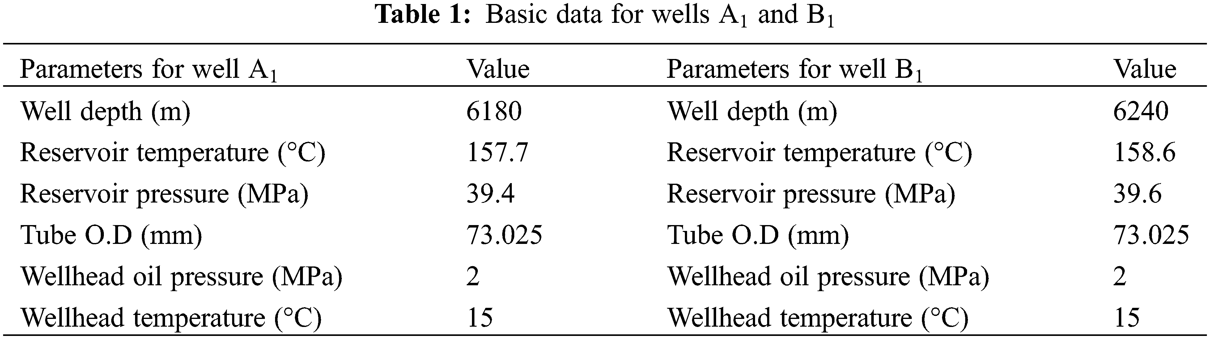
The reservoir and production parameters of wells A1 and B1 in the W shale gas field are shown in Table 1.
The OLGA software simulation sets the DTPLOT (animated simulation step) to 100 s. The minimum pipe section length of the grid division is 50 m, and the maximum pipe section length is 500 m. The time iteration step is taken to be 0.01 s, and the maximum time iteration step and the minimum time iteration step are taken to be 100 s and 0.001 s, respectively.
3 Simulation Study of Production Dynamics in Deep Shale Gas Wells
3.1 Gas-Liquid Flow Mechanism Analysis
Theory of Minimum Pressure Drop
From the analysis of a large number of theoretical studies, it is known that the pressure drop in gas-liquid two-phase flow consists of two main components (the friction pressure drop and the gravity pressure drop). Under the condition of low gas velocity, the total pressure gradient decreases with the increase of gas velocity. When the gas flow rate is greater than a certain critical value, the wellbore basically does not produce fluid accumulation, at this time, with the increase of gas velocity, the total pressure gradient continues to increase, so in the whole process of gas flow rate increase, there is a minimum value of pressure gradient in the wellbore, and at this time the corresponding gas flow rate is the critical flow rate [24].
(1) Gas-liquid homogeneous flow
When the gas flow rate is relatively large, the center gas core and the liquid film on the tube wall move upward at the same time, at this time, the flow pattern in the wellbore is the ring mist flow, the force in the wellbore is shown in Fig. 2a, in which the shear stress between the liquid film and the gas core is τI direction upward along the wall of the tube, and the shear stress between the liquid film and the tube wall is τw along the wall of the tube downward, and the force of their own gravity G and The tube wall force on the liquid film N. As the gas flow rate increases, the shear stress between the gas and the liquid film τi is greater, and the friction pressure drop in the tube is greater; at the same time, due to the increase in gas velocity, the liquid phase entrainment in the gas core increases, and the density of the mixture increases, resulting in an increase in the gravitational pressure drop in the direction of the tube wall, and the gravitational component perpendicular to the wall increases, which then increases the shear stress between the liquid film and the tube wall τw. Therefore, the gradient of pressure drop in the wellbore gradually increases as the gas flow rate increases.
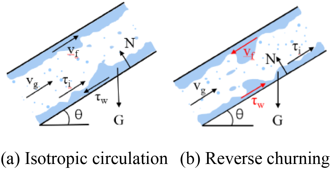
Figure 2: Mechanical analysis: (a) Isotropic circulation and (b) reverse churning
(2) Reverse gas-liquid flow
When the gas flow rate is relatively small, due to the reason of gravity, the gas-liquid flow occurs in the reverse direction due to slippage. At this time, the flow pattern in the wellbore is churning flow, and the force in the wellbore is shown in Fig. 2b. Among them, the gas-liquid interface shear stress τi, the shear stress of the liquid film and the tube wall τw direction is upward along the tube wall, its own gravity G and the tube wall support force on the liquid film N. As the gas flow rate decreases, the liquid film slips off the more serious, and the liquid film gradually becomes thicker; due to the further decrease in the cross-section of the gas passing through the liquid film, which makes the gas flow rate increase compared with the previous one, and the total pressure drop increases eventually. As the thickness continues to increase, both the friction pressure drop and gravity pressure drop increase, so the total pressure drop increases.
(3) Fluid membrane arrest
When the gas changes from high flow rate to low flow rate, there is a critical state where the liquid film changes from upward motion to downward motion, at which time the liquid film is stagnant and the flow pattern in the wellbore is an annular mist flow. In this state, because the liquid film does not move, so the liquid film and the wall of the shear stress is zero, at this time the pressure drop in the wellbore is minimized, corresponding to the gas flow rate that is the critical flow rate.
(4) Gas-liquid flow when tubing is at different locations in the wellbore
When tubing is lowered into the wellbore, the diameter of the section of tubing between the wellhead and the end of the wellhead and tubing is equal to the inner diameter of the tubing, while the diameter of the remaining section of tubing is equal to the inner diameter of the casing. When the cross-section of the fluid flow decreases, the flow rate increases accordingly, which helps the gas to carry the fluid, but at the same time increases the friction loss, as shown in Fig. 3a.
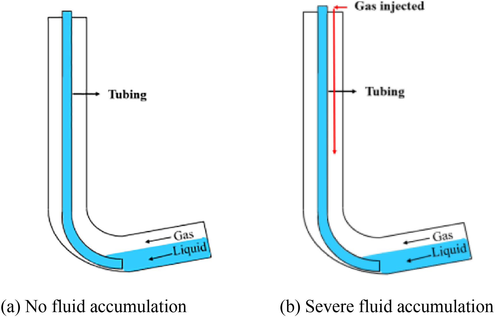
Figure 3: Schematic diagram of gas-liquid flow down the tubing into the wellbore: (a) No fluid accumulation and (b) severe fluid accumulation
In actual production, there is a relationship between the gas flow rate and the bottomhole flow pressure, known as the inflow dynamic curve (IPR). The purpose of the preferred tubing optimal lowering position is to generate higher gas production from the reservoir, rather than using minimum pressure drop as an optimization parameter. This is because when a fluid accumulation situation occurs in a horizontal section, the horizontal section is not highly inclined, resulting in insignificant wellbore backpressure due to gravity factors. Therefore, when fluid accumulation occurs at a certain location, it may be less effective to occur through the minimum pressure drop.
When the flow rate is very large gas flow, gas-liquid ratio is also relatively large, liquid accumulation can be ignored, the optimal depth of the oil pipe in the horizontal section of a certain place does not need to go down to the lowest end, which can ensure that the pressure drop of the whole section of the minimum pressure drop, but also do not need to go down into the oil pipe to the deepest position. When the flow rate decreases, the optimal depth of the oil pipe at a certain place according to the minimum pressure drop in the whole pipe section may have flow safety and security problems, in order to avoid this situation, the oil pipe needs to be lowered into the toe end, to avoid the collection of liquid. When the flow rate continues to decrease, even at the toe end, there is no guarantee of the liquid accumulation problem, and it may not be possible to eliminate the accumulation of liquid, and then the problem should be analyzed in conjunction with the air-lift process, as shown in Fig. 3b.
3.2 Model Rationality Validation
OLGA considers two basic flow types: separated flow and dispersed flow, the former subdivided into stratified flow and annular flow, and the latter subdivided into dispersed bubble flow and segmented plug flow.
In the simulation process, the shale gas development process is regarded as a decaying extraction process, and the change of reservoir pressure during the production process is reflected by the decrease of formation pressure with the production time, which ignores the influence of the horizontal section fluid inflow location, the change of reservoir permeability, and desorption and other influencing factors [25]. The fitting results obtained when the gradient of formation pressure decrease with time is 0.06 MPa/d show that the software simulation results are basically consistent with the trend of actual production data, and the results are shown in Fig. 4. In order to better demonstrate the rationality of the method, four more production wells from the same platform were simulated. The feasibility of the method can be found by comparing the production of the simulated wells with that of the actual production wells.
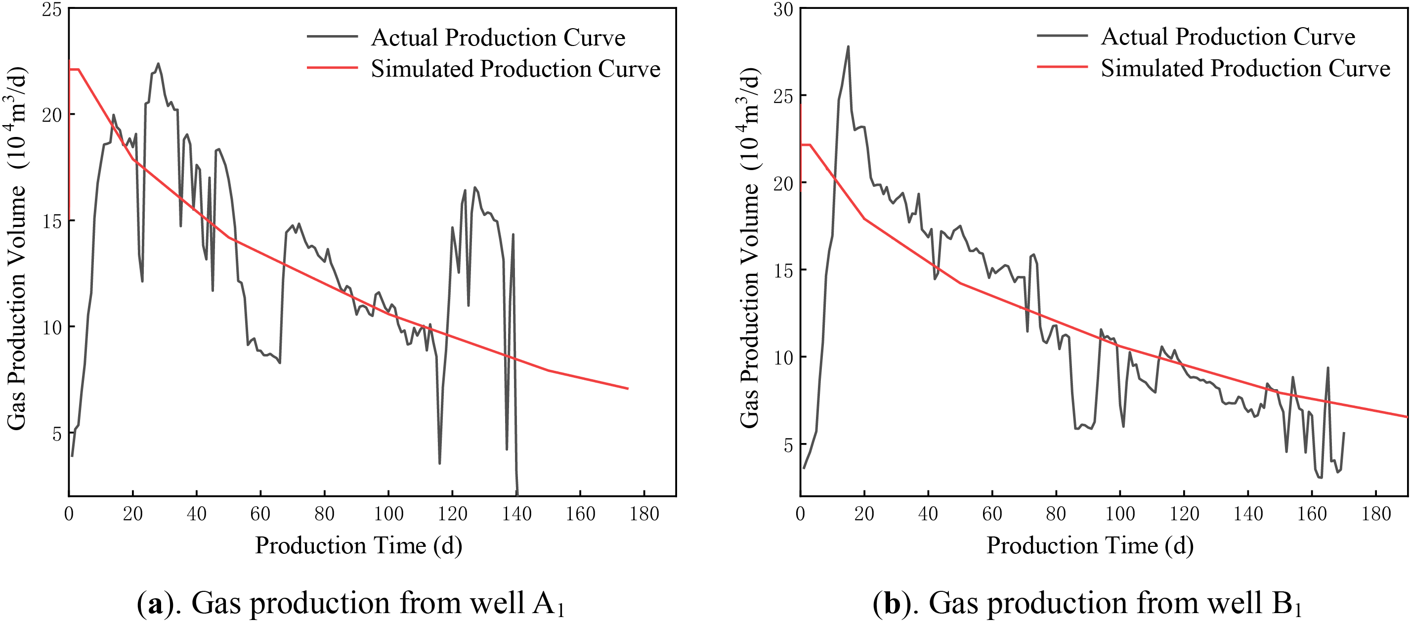
Figure 4: Comparative analysis of actual production and simulation results
Due to the long actual production time, simulating a single operating condition based on real circumstances would take 4 days or even longer. In order to speed up the simulation time, the gradient of formation pressure drop with time was increased by a factor of 24 for all simulations, and the pressure drop gradient was set to 0.06 MPa/h. As can be seen from Fig. 5, the results of numerical simulation are within 10% of the actual error. Therefore, the later simulation by shortening the time is somewhat reasonable and feasible.
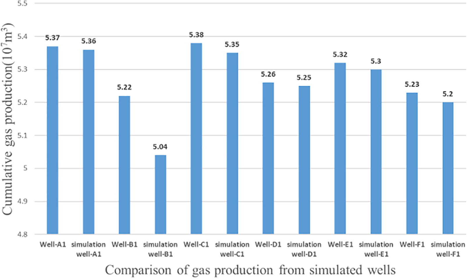
Figure 5: Comparison of gas production from simulated wells
3.3 Dynamic Simulation under Various Well Trajectory Conditions
Study into the dynamic characteristics of gas-liquid flow in gas wellbores is essential for assessing the production performance of gas wells [26]. Consequently, simulations of liquid carryover and subsequent liquid accumulation in water-producing gas wells should be as consistent as possible with actual conditions. In gas well production, the fluid generally flows For normal production of gas well production, it is easy to produce stratified flow in the horizontal section and annular flow in the vertical section and the slope-making section. This is because of the gravity of the liquid, in the horizontal section the direction of gravity is perpendicular to the gas-liquid flow direction, while in the vertical section, the direction of gravity is opposite to the flow direction, as depicted in Figs. 6 and 7. Due to the differences in the inclination angle of the horizontal section, the fluid flow in the horizontal section of shale gas wells with different trajectory paths exhibits varying flow patterns and changes.
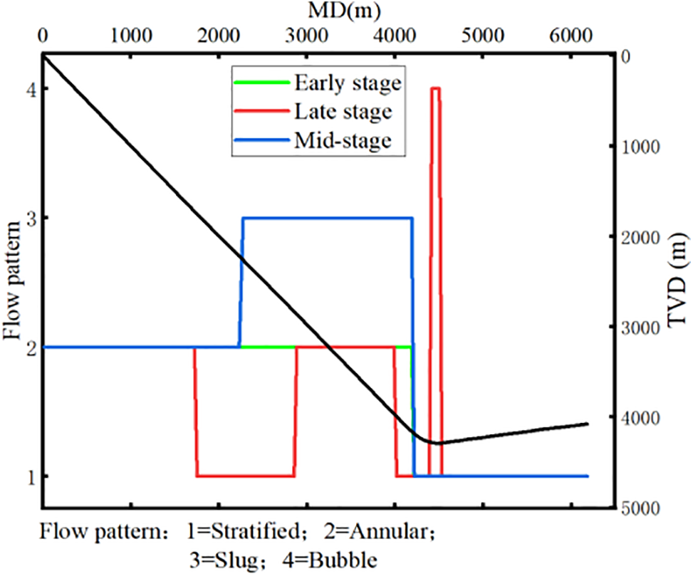
Figure 6: Flow regime diagrams for well A1 at various production stages
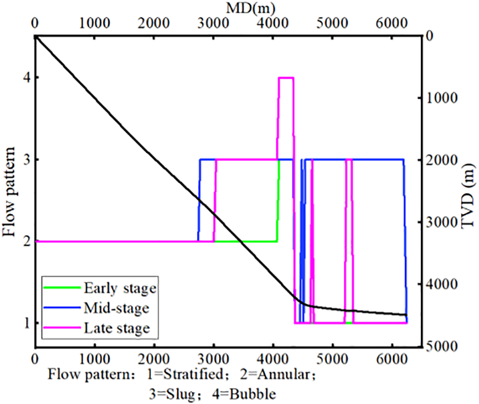
Figure 7: Flow regime diagrams for well B1 at various production stages
For wells A1 with an upward-tilted horizontal section and well B1 with a downward-tilted horizontal section, during the mid-to-late production stage, slug flow occurs at the build-up section, with liquid accumulation most likely to happen at this section [27]. As the wellhead production pressure gradually decreases, the flow regime in various sections of the wellbore changes, as shown in Figs. 6 and 7. When the gas-liquid fluid mixture in the wellbore occurs plugging flow as it rises, When the gas-liquid mixture rises in the wellbore and exhibits slug flow, it results in alternating segments of liquid and gas. As the liquid column ascends with insufficient energy, slippage losses occur, causing the liquid to accumulate at the bottom. With the increase in backpressure at the bottom, a new cycle of slug flow initiates, carrying the pooled liquid to the surface. Subsequently, as the bottom pressure decreases, the liquid column once again falls back to the well bottom [28,29]. The primary cause of slug flow is the decrease in formation pressure. The key difference between the two distinct well trajectories is that horizontal sections with an upward bend only exhibit slug flow in the inclined zone, whereas horizontal sections with a downward bend can also occur slug flow. The reason is that when the horizontal section is inclined upwards, the alignment of the fluid flow direction with gravity results in the liquid’s gravity performing positive work, even in cases of gas-liquid slippage, to increase the velocity of the liquid phase. As depicted in Fig. 8, the gas production of shale gas wells with an upwardly inclined horizontal section is generally higher than that of wells with a downwardly inclined horizontal section. Moreover, under the same production conditions, wells with a downwardly inclined horizontal section are more prone to liquid accumulation.
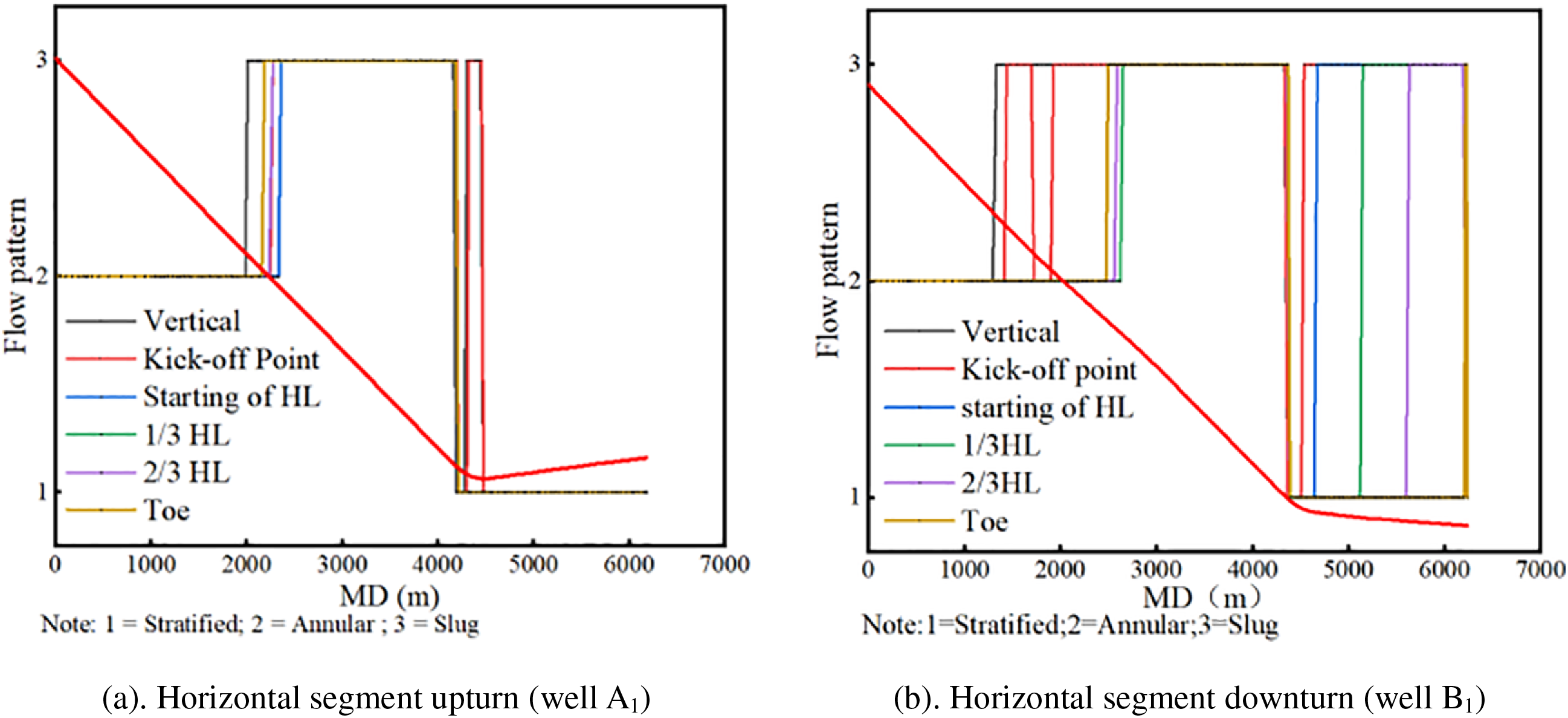
Figure 8: Changes in flow patterns in the middle and late stages of production
3.4 Dynamic Simulation for Different Tubing Depths
With the deepening insertion of the tubing into the wellbore, the fluid conduit diameter decreases, which while enhancing the gas well’s liquid-carrying capacity, also leads to an increase in frictional resistance throughout the flow path [30]. Variations in tubing depth cause alterations in fluid velocity, pressure, and temperature within the tubing and casing, impacting the flow dynamics at different positions along the tubing. The simulation results of six different physical models for tubing depth indicate that when the tubing is placed at the Heel position, the zone of segmented flow in the KOP section is minimized, and it is less prone to liquid accumulation compared to other positions. Bubble flow emerges in the late production stage, with the formation of bubbles caused by the increased back pressure at the well bottom due to the rising liquid column height, as the gas in the liquid phase breaks free from its constraints, as depicted in Figs. 6–8.
Fig. 9 illustrates that cumulative production decreases with increasing tubing depth, yet the tubing’s placement in the horizontal section significantly influences production yield. Fig. 10 reveals that for well A1 with an upward-sloping horizontal section, the lag in liquid accumulation increases with deeper tubing placement. This is attributed to the reduced flow area as tubing depth increases, which elevates gas velocity and decreases the critical liquid-carrying flow rate, thereby slowing the accumulation of liquid. For deep well B1 with a downward-sloping horizontal section, the time for liquid accumulation first increases and then decreases with the depth of tubing insertion, with a peak value occurring at 1/3HL (Horizontal segment at 1/3) along the horizontal section. In deep wells with a downward-sloping horizontal section, liquid accumulation is most likely to occur at the vertical section where the tubing is inserted, while it is least likely to happen at the 1/3HL position in the horizontal section. Therefore, for deep shale gas wells, if the horizontal section is upward-sloping, placing the tubing at the point where the KOP section is most beneficial for production, as it ensures the highest gas production rate and delays the time for liquid accumulation in the wellbore. Conversely, if the horizontal section is downward-sloping, placing the tubing at the Heel section is most advantageous for production. The fluid accumulation patterns differ between wells A1 and B1 as follows: (a) In deep well A1 with an upward-tilted horizontal section, fluid accumulation is postponed as the tubing depth increases. (b) In deep well B1 with a downward-tilted horizontal section, deeper tubing does not necessarily delay fluid accumulation; rather, from the vertical section to the 1/3HL position in the horizontal section, the onset of fluid accumulation initially increases, and from the 1/3HL position to the toe, the accumulation time decreases progressively with increased tubing depth. The 1/3HL position is the least susceptible to fluid accumulation. A commonality in both patterns is the propensity for fluid accumulation when the tubing is inserted into the vertical section.
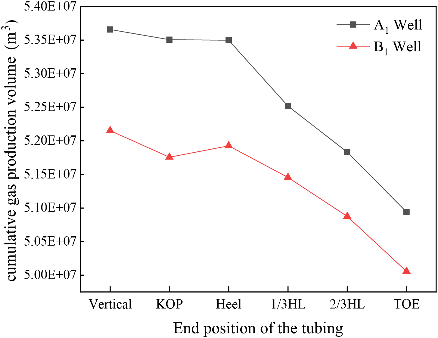
Figure 9: Tubing position impact on gas yield in deep wells
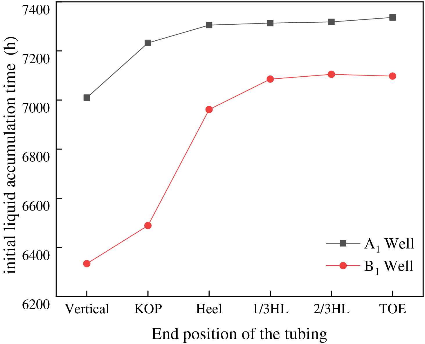
Figure 10: Variation in liquid accumulation time with tubing placement
Production analysis indicates that the deep well with an upward-tilted horizontal section is superior to the deep well with a downward-tilted horizontal section. This is due to the consistently higher production and longer normal production duration with later fluid accumulation in the upward-tilted well, regardless of the tubing position. Therefore, for well A1 with an upward-tilted horizontal section, it is recommended to lower the tubing to the KOP zone. For well B1 with a Heel horizontal section, it is suggested to position the tubing at the toe of the horizontal section, as adopting an upward-tilted horizontal section for gas well production is more economical.
3.5 Dynamic Simulation Study under Varying Well Depth Conditions
The effect of shale gas well depth on gas-liquid flow, with the main influencing factors being temperature and pressure. Gases also have expansion energy during output. As depth increases, the gas’s expansion energy and flow rate intensify, enhancing the ability to carry liquids, thereby reducing the likelihood of fluid accumulation in the wellbore and extending the production time of the gas wells [31].
3.5.1 Horizontal Section Upturned Well
With the tubing positioned at the heel end of the horizontal zone, the deep well’s production is approximately 1.94-fold that of a conventional well, reflecting a production rise of 2.597 × 10⁴ m3/m with depth. Additionally, the normal production duration is roughly 1.30 times that of a conventional well, with an increase of 2.2 h/m as depth increases.
In terms of production, when the tubing is lowered into the vertical section to the heel end of the horizontal section, the conventional wells and deep wells do not have the same change in production, in which the production of conventional wells increases with the increase of the depth of tubing, and the production of deep wells decreases with the increase of the depth of the tubing, and the trend of change of the two wells is exactly the opposite. When the tubing is lowered into the horizontal section from the heel end to the toe end position, the conventional wells and deep wells have the same production change, and the production decreases with the increase of the tubing depth, as shown in Fig. 11a.
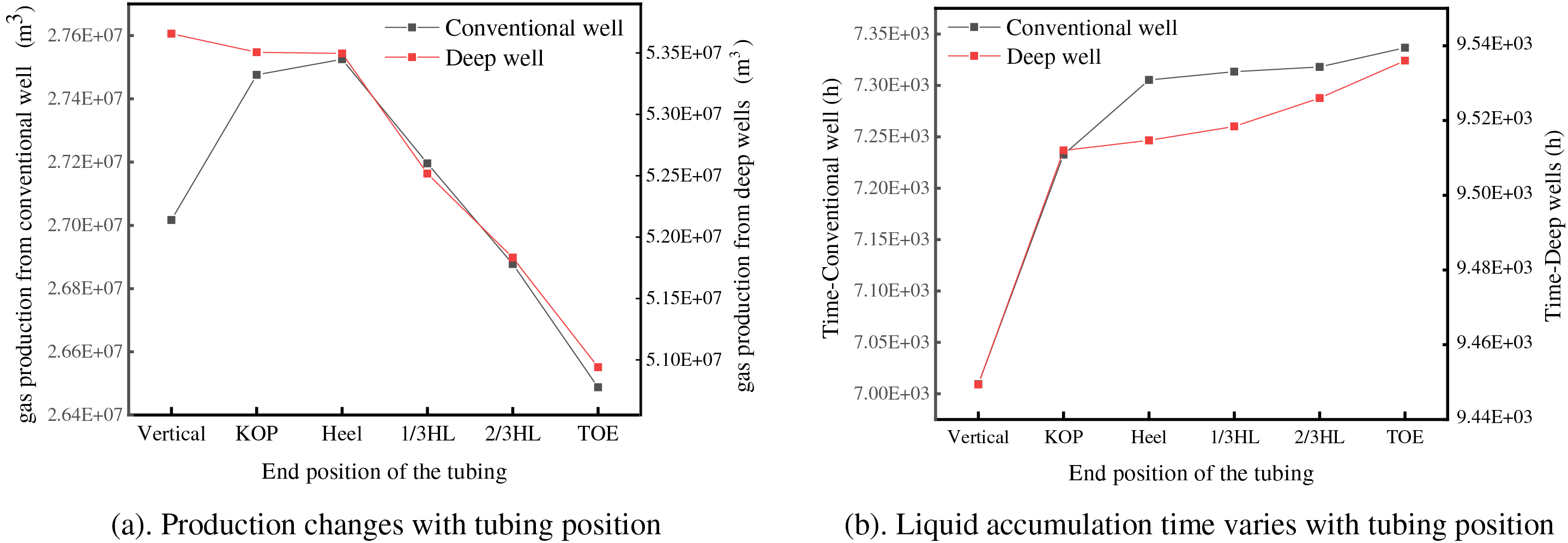
Figure 11: Comparison of horizontal section upturned deep wells and conventional wells
In terms of water accumulation, the trend is consistent between conventional and deep wells. As the depth of the tubing increases, the less likely it is to accumulate fluid. However, the difference is that the magnitude of change is not the same from the KOP section to the toe position, and the effect of tubing depth in deep wells on the time of fluid accumulation is larger than that of conventional wells, as shown in Fig. 11b.
3.5.2 Horizontal Section Downturned Well
When the tubing are lowered into 1/3HL position of the horizontal section, the production of the deep well is about 1.87 times of the production of the conventional well, i.e., the production corresponds to an increase of 2.395 × 10⁴ m3/m with the increase of depth; and the time of normal production is about 1.34 times of the time of production of the conventional well, i.e., the time of normal production increases by 2.4 h/m with the increase of depth.
In terms of production, overall, with the increase of tubing depth, the two kinds of wells have the same trend of production change with well depth, which is firstly decreasing, then increasing and then decreasing. The difference is that for conventional wells, there is a great value at 1/3 HL in the horizontal section and the production is the maximum value; while deep wells do not have a maximum value point and the production is the largest in the sloping section, as shown in Fig. 12a.
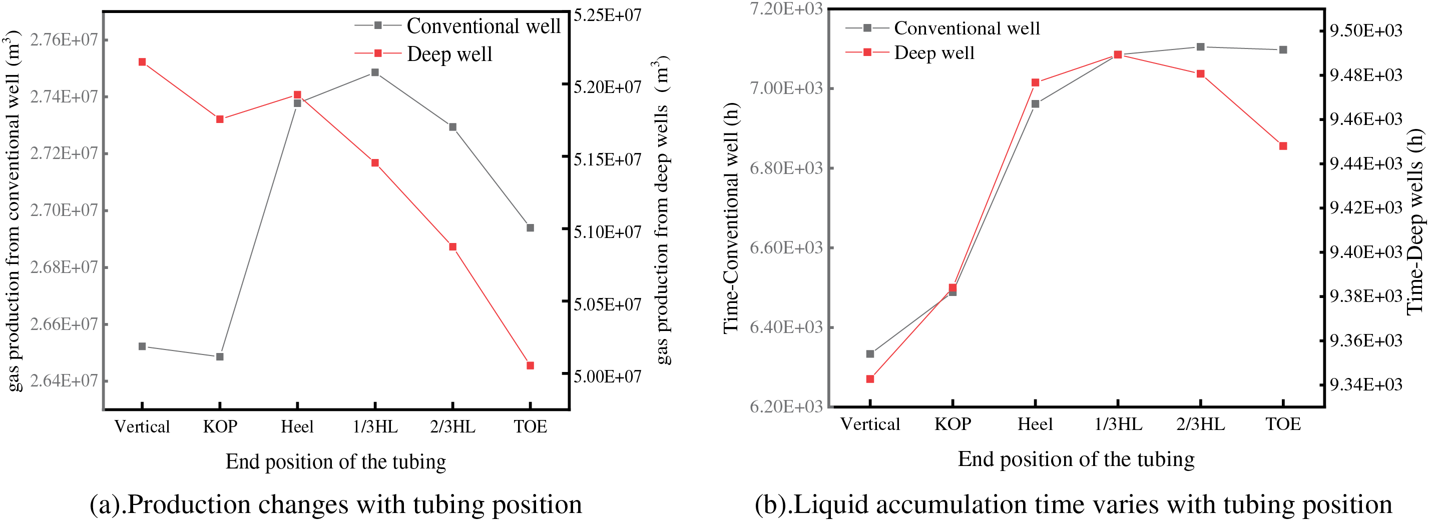
Figure 12: Comparison of horizontal section downgradient deep wells and conventional wells
In terms of water accumulation, both conventional and deep wells exhibit a consistent trend of initial increase followed by a decrease in fluid accumulation. The distinction lies in the tubing position with the least likelihood of accumulation: for conventional wells, it is at 2/3 of the horizontal section (2/3HL), where deeper tubing results in a diminished impact on fluid accumulation. In contrast, for deep wells, the minimum accumulation occurs at 1/3HL, and below this position, fluid accumulation exhibits significant changes. This is illustrated in Fig. 12b.
The analysis reveals that the optimal tubing depth placement differs between conventional and deep wells, with deep wells being more beneficial for production increase. For conventional shale gas wells with an upsloping horizontal section, tubing placement at the horizontal segment heel is more appropriate, while for deep shale gas wells, placement in the KOP section is preferable. In the case of a downsloping horizontal section, conventional wells should place the tubing at 1/3 of the horizontal length (1/3HL), whereas deep wells are better served by placing the tubing at the horizontal segment heel.
4 Conclusion and Recommendations
The study demonstrates that proper tubing depth placement can significantly impact production performance and liquid accumulation in deep shale gas wells. Upward-buckled horizontal sections generally perform better than downward-inclined sections. Deep wells show considerable advantages over conventional wells in terms of production and normal production duration.
1. For deep shale gas wells with upward-buckled horizontal sections, place tubing at the Kick-off Point position.
2. For deep shale gas wells with downward-inclined horizontal sections, place tubing at the heel of the horizontal section.
3. When possible, prefer well designs with upward-sloped horizontal sections for better production and reduced fluid accumulation risks.
This research provides valuable insights for optimizing deep shale gas well designs and production strategies, potentially leading to improved efficiency and economic performance in deep shale gas extraction operations.
Acknowledgement: I would like to thank Editor of the FDMP Journal for his guidance and assistance in revising this paper.
Funding Statement: The authors received no specific funding for this study.
Author Contributions: The authors confirm contribution to the paper as follows: study conception and design: Jie Liu; analysis and interpretation of results & article writing: Sheng Ju. All authors reviewed the results and approved the final version of the manuscript.
Availability of Data and Materials: As part of the data in the content is field data, oilfield confidentiality is not divulged. In addition, if you need the simulated data, you can contact the author by emailing.
Ethics Approval: Not applicable.
Conflicts of Interest: The authors declare no conflicts of interest to report regarding the present study.
References
1. Altwaijri M, Xia Z, Yu W, Qu L, Hu Y, Xu Y, et al. Numerical study of complex fracture geometry effect on two-phase performance of shale-gas wells using the fast EDFM method. J Pet Sci Eng. 2018;164(5):S0920410517310495. [Google Scholar]
2. Liu SB, Wang DF, Liu L, Zhang XD, Li P. Research on drainage gas production technology of extended reach horizontal well by coiled tubing. Natural Gas and Oil. 2022;40(6):61–8. [Google Scholar]
3. Wang QR, Chen JX, Cai DG, Yang Z, Chen K. Research and application of production string optimization in shale gas wells. Natural Gas Oil. 2022;40(1):72–6. [Google Scholar]
4. Osman E. S. A. Prediction of critical gas flow rate for gas wells unloading. Soc Petrol Eng. 2002. doi:10.2118/78568-MS. [Google Scholar] [CrossRef]
5. Johri N, Kadam S, Veeken K, Prakash A, Suvarna H, Singh P, et al. Conquer liquid loading in Raageshwari gas field by automated intermittent production and deliquification. In: Abu Dhabi International Petroleum Exhibition and Conference, 2023 Oct 02; Abu Dhabi, United Arab Emirates. [Google Scholar]
6. Mccoy JN, Rowlan OL, Podio A. Acoustic liquid level testing of gas wells. In: SPE Production and Operations Symposium, 2009 Apr; Oklahoma. [Google Scholar]
7. Veeken C, Al Kharusi D. Selecting artificial lift or deliquification measures for deep gas wells in the sultanate of Oman. In: SPE Kuwait Oil & Gas Show and Conference, 2019; Mishref, Kuwait. [Google Scholar]
8. Bahadori A, Zahedi G, Zendehboudi S, Jamili A. A simple method to estimate the maximum liquid production rate using plunger lift system in wells. Nafta. 2012;63(11–12):365–9. [Google Scholar]
9. Uddin MFM, Tayyab I, Koondhar NH, Ahmed QI, Soomro AA. Production optimization of foam assisted lift (FAL) wells and evaluation of good and bad practices to ensure maximum production. In: SPE/PAPG Pakistan Section Annual Technical Conference, 2015 Nov; Islamabad, Pakistan. [Google Scholar]
10. Alshmakhy A, Bigno Y, Saqib T, Soomro M, Faustinelli J, Faux S, et al. Digital intelligent artificial lift DIAL gas lift production optimization deployments across assets. In: SPE Annual Technical Conference and Exhibition, 2021 Sep; Dubai, UAE. [Google Scholar]
11. Flores-Avila FS, Riano JM, Javier-Martinez M, Hammond T, Cantu J, Ramos J. New artificial lift system using coiled tubing and reciprocating downhole pumps for heavy and viscous oil. In: SPE Latin America and Caribbean Petroleum Engineering Conference, 2012 Apr; Mexico. [Google Scholar]
12. Du Y, Lei W, Li L, Zhao ZJ, Ni J, Liu T. Production management and drainage technology of deep shale gas horizontal wells after pressure. Reservoir Eval Dev. 2021;11(1):95–101+116. [Google Scholar]
13. Luo CC, Wu N, Wang H, Liu YH, Zhang T, W. BQ, et al. Flow pressure drop prediction of gas-liquid two-phase pipe in horizontal gas well. J Shenzhen Univ (Sci Technol Ed). 2022;39(5):567–75. [Google Scholar]
14. Beggs D, Brill JP. A study of two-phase flow in inclined pipes. J Petrol Technol. 1973;25(5):607–17. doi:10.2118/4007-PA. [Google Scholar] [CrossRef]
15. Hewitt GF, Roberts DN. Studies of two-phase flow patterns by simultaneous X-ray and flash photograph. AERE-M2159; 1969. Available from: https://www.osti.gov/biblio/4798091. [Accessed 2024]. [Google Scholar]
16. Asghar A, Masoud R, Jafar S, Abdulaziz Alsairafi A. CFD and artificial neural network modeling of two-phase flow pressure drop. Int Commun Heat Mass Transf. 2009;36(8):850–6. doi:10.1016/j.icheatmasstransfer.2009.05.005. [Google Scholar] [CrossRef]
17. Deendarlianto MA, Adhika W, Dinaryanto O, Khasani I. CFD studies on the gas-liquid plug two-phase flow in a horizontal pipe. J Petrol Sci Eng. 2016;147(2):779–87. doi:10.1016/j.petrol.2016.09.019. [Google Scholar] [CrossRef]
18. Mandhane JM, Gregory GA, Aziz K. A flow pattern map for gas-liquid flow in horizontal pipes. Int J Multiphase Flow. 1974;1(4):537–53. doi:10.1016/0301-9322(74)90006-8. [Google Scholar] [CrossRef]
19. Cheng Y, Wu RD, Liao RQ, Liu ZL. Study on calculation method for wellbore pressure in gas wells with large liquid production. Processes. 2022;10(4):685. doi:10.3390/pr10040685. [Google Scholar] [CrossRef]
20. Salim PH, Li J. Simulation of liquid unloading from a gas well with coiled tubing using a transient software. In: SPE Annual Technical Conference and Exhibition, 2009 Oct; New Orleans, LA, USA. [Google Scholar]
21. Zhang LS. Experimental study and transient numerical calculation of gas-liquid two-phase pipe flow. China: Wuhan University; 2020. [Google Scholar]
22. Pang B, Li ZM, Wu JJ, Xu SY, Chen WX. Numerical simulation of gas-liquid two-phase flow in deep coalbed methane horizontal wellbore. Coal Technol. 2024;43(10):48–2 (In Chinese). [Google Scholar]
23. Guo YD. A shale gas well production prediction method based on material balance equation. China Min Ind. 2018;27(6):153–9. [Google Scholar]
24. Shen WW, Deng DM, Liu QP. Prediction model of critical flow rate in gas wells based on annular mist flow theory. J Chem Eng. 2019;70(4):1318–30. [Google Scholar]
25. Wang YH, Che MG, Wang M, Liu J, Liao RQ. Influence of tubing depth on drainage effect of horizontal shale gas well. J Yangtze Univ (Natur Sci Ed). 2021;18(3):49–59. [Google Scholar]
26. Huang WM, Wang JQ, Zhang N, An ZB, Wang QB. Optimization method of production parameters of plunger row based on transient simulation. Oil Drill Prod Technol. 2022;44(5):589–93. [Google Scholar]
27. He YQ, Chen Q, Wu TT, Zeng LJ, Wang YT, Luo X, et al. Research on wellbore accumulation flow law of shale gas horizontal wells: a case study of well C01. Oil Gas Chem Ind. 2022;51(2):77–82 (In Chinese). [Google Scholar]
28. Atr R, Sarica C, Pereyrae E. End of tubing (EOT) placement effects on the two-phase flow behavior in horizontal wells: experimental study. In: SPE Annual Technical Conference and Exhibition, 2016 Sep; Dubai, United Arab Emirates. [Google Scholar]
29. Dinata RC, Sarica C, Pereyra EA. Methodology of end of tubing EOT location optimization for horizontal shale gas wells with and without deliquification. In: SPE North America Artificial Lift Conference & Exhibition, 2016 Oct 25–27; Woodlands, TX, USA. [Google Scholar]
30. Du Y, Ni J, Lei W, Zhou XF, Li L, Bu T. Research on optimal tubing parameters design of Weirong deep shale gas well. Reservoir Eval Dev. 2022;12(3):526–33. [Google Scholar]
31. Luo S, Kelkar M, Pereyra E, Sarica C. A new comprehensive model for predicting liquid loading in gas wells. SPE Prod Oper. 2014;29(4):337–49. [Google Scholar]
Cite This Article
 Copyright © 2025 The Author(s). Published by Tech Science Press.
This work is licensed under a Creative Commons Attribution 4.0 International License , which permits unrestricted use, distribution, and reproduction in any medium, provided the original work is properly cited.
 Downloads
 Citation Tools