The Influence of an Imposed Jet and Front and Rear Wall Modification on Aerodynamic Noise in High-Speed Train Cavities

1  Introduction

With the rapid development of the railway system, the interconnection between high-speed railways and residents along the line is becoming increasingly close. However, as the speed of high-speed trains continues to increase, the noise generated by them has already affected the normal lives of residents along the line. Therefore, controlling the noise generated by high-speed trains is a key issue that needs to be addressed to facilitate further speed enhancements.

Extensive research has been conducted to identify the sources of noise associated with high-speed trains, with findings indicating that the noise can be primarily categorized into two types: wheel-rail noise and aerodynamic noise [1–4]. It is established that once trains exceed speeds of 300 km/h, aerodynamic factors become the predominant source of external noise radiation [5,6]. The pantograph, which serves multiple functions, experiences substantial interaction with the incoming air during high-speed operation, leading to considerable pressure fluctuations on its surface [7–9]. In addition, during the train’s operation, the interaction between the incoming air and the pantograph cavity can also generate intense aerodynamic noise, so the aerodynamic noise produced by the pantograph cavity should not be ignored [10].

Many scholars have conducted in-depth research on the aerodynamic noise generated by the interaction between the incoming air and the pantograph cavity. Kim et al. [11] found that the flow separation at the cavity’s leading-edge results in detached gas, which increases pressure fluctuations on the cavity’s rear wall, consequently generating additional noise. Tan et al. [12] conducted numerical simulation analysis of the pantograph area and aerodynamic noise simulation calculations, revealing that over 50% of the total sound source energy was concentrated in the lower part of the pantograph. From these studies, it can be observed that the aerodynamic noise generated by the pantograph cavity itself is very significant, and effective measures must be taken to control it. In their efforts to mitigate this noise, Yu et al. [13] studied aerodynamic noise in an open cavity at a Mach number of 0.85. Their findings indicate that merely altering the direction and intensity of the shear layer is inadequate for reducing the sound source intensity within the cavity. They emphasize the importance of altering the stability of the shear layer to effectively influence both the distribution and strength of the sound sources. Saddington et al. [14] conducted experiments on the effects of cavity front and rear wall modifications and spoilers on cavity flow at a Mach number of 0.71. The results of their study suggest that leading-edge control technologies are more effective than trailing-edge modifications in alleviating aerodynamic noise.

Araddag et al. [15] studied modifications to the cavity’s rear wall and discovered that, under supersonic flow conditions, such alterations effectively mitigates the aerodynamic noise produced by the cavity. Kim et al. [16,17] found that by modifying the edges of the cavity with rounded and chamfered edges, the radiation noise of the cavity can be reduced. Yu et al. [18] further contributed to this area of research by analyzing the impact of jets on cavity noise. In their study, they mentioned that jets can raise the height of the shear layer above the cavity, thereby reducing the air flow velocity inside the cavity and weakening the noise radiated by the cavity. Zhang et al. [19] investigated the application of a jet at the leading edge of the cavity as a strategy for minimizing aerodynamic noise within pantograph cavities. Their results revealed that adding a jet at upstream of the cavity can effectively reduce the turbulent kinetic energy amplitude and vortex structure in the cavity, thus realizing the reduction of aerodynamic noise radiated by the cavity. Ukai et al. [20] explored the effect of different positions of the jet on the noise radiated by the cavity under high Mach velocity conditions. In their study, it was found that the presence of the jet made the flow above the cavity unstable, which might be improved if combined with front and rear wall tilt trimming.

The literature review indicates that current research on passive control methods involving modifications to the front and rear walls of cavities predominantly addresses cavity flow at higher Mach numbers. In contrast, studies focusing on inclination modifications of cavity walls at lower Mach numbers are considerably limited. Additionally, investigations concerning the active control of jets similarly emphasize cavities operating at elevated Mach numbers, while there is a notable lack of inquiry into the effects and mechanisms of aerodynamic noise in cavities under the typical operating conditions of high-speed trains. Furthermore, there is a scarcity of research investigating the effect of varying jet velocities on aerodynamic noise within the cavity. Thus, this paper seeks to investigate the impact of varying jet velocities on the aerodynamic noise of the cavity at typical high-speed train operating speeds and to identify the underlying patterns of this influence. By simultaneously applying active jet control and passive modifications to wall inclination, the study aims to mitigate surface pressure pulsation amplitudes within the cavity area. The related research work in this paper provides valuable ideas and techniques for reducing the aerodynamic noise generated by the pantograph cavity of high-speed trains and is expected to contribute to the development of noise control technology in this field.

2  Numerical Methods

To ensure the accuracy of numerical calculations, it is necessary to choose appropriate methods for numerical simulation. This article employs the Improved Delayed Detached-Eddy Simulation (IDDES) method based on SST k-w to simulate the flow field in the cavity region. Specific details about the IDDES model can be found in references [21–23]. In terms of acoustic simulation, the aerodynamic noise generated in the cavity area is calculated based on the FW-H equation. The FW-H equation, derived from the Navier-Stokes (N-S) equations, is used to assess the aerodynamic noise produced by solid surfaces. In acoustic calculations, the right-hand side of the equation is utilized as the sound source term [24]. Due to the complexities associated with direct solutions of the FW-H equation, a simplification must be undertaken to facilitate acoustic analysis.

In the acoustic framework provided by the FW-H equation, the first term on the right side of the equation is the monopole sound source term generated by periodic motion, the second term is the dipole sound source term generated by surface pressure pulsation, and the third term is the quadrupole sound source term generated by turbulent stress in the flow field. The total source of aerodynamic noise generated by an object is the sum of the three terms on the right-hand side of the equation. As shown in Eq. (1).

p′(x,t)=pT′(x,t)+pL′(x,t)+pQ′(x,t)(1)

where pT′(x,t), pL′(x,t) and pQ′(x,t) represent the monopole sound source term generated by periodic motion, the dipole sound source term generated by surface pressure pulsation, and the quadrupole sound source term generated by turbulent stress, respectively.

The research conclusions of references [25,26] indicate that under low Mach number flow conditions, the noise generated by the quadrupole contributes very little to the overall noise, and therefore can be ignored in acoustic simulations of the pantograph region. Meanwhile, Zhao et al.’s [27] research results indicate that for the pantograph area of high-speed trains, the aerodynamic noise contributed by dipoles is much greater than that contributed by quadrupoles. Therefore, this study excludes the fourth-order sub sound source term from its acoustic simulation calculations. For the monopole source term, the cavity remains stationary during numerical calculations, so the surface velocity of the cavity is 0. Thus, the monopole source term based on periodic motion is also 0. Given these considerations, this study focuses solely on the dipole sound source resulting from pressure pulsations on the surface of the cavity during the acoustic simulation. For the dipole source term, Farassat developed a time-integrated solution of the FW-H equation applicable to subsonic flow conditions, which is suitable for numerical analyses [28]. Therefore, this method is used for all numerical simulation cases in this study regarding the far-field noise prediction in the pantograph cavity. The formula for calculating the sound pressure contributed by a dipole source is as follows:

pL′(x,t)=14πc0∫[L⋅rr(1−Mr)2]retdS+14π∫[Lr−LMr2(1−Mr)2]retdS+14πc0∫[Lr(rM⋅r+c0Mr−c0M2)r2(1−Mr)3]retdS(2)

Li=Pijnj+ρui(un−vn)(3)

Pij=(p−p0)δij−σij(4)

where Mi is the Mach number in the xi direction and Mr is the Mach number in the observer direction, the subscript ret of the integral term represents the evaluation of the relevant variable over time, c0 is the speed of sound, r is the distance from a source point to the observer, un is the fluid velocity component normal to the surface, vn is the surface velocity component normal to the surface, Pij is the compressive stress tensor, σij is the viscous stress tensor, and p0 is the ambient pressure.

3  Numerical Model

3.1 Geometric Model

The computational model used for numerical simulations in this study features a clean cavity, free of any internal objects, with dimensions of Length L = 427 mm, Depth D = 61 mm, and Width W = 305 mm. The structure conforms to a typical open cavity [29]. The geometric characteristics of the cavity closely resemble those of the actual pantograph area cavity found on high-speed trains. At the forefront of the cavity, a jet slot measuring 3 mm in width is strategically positioned, with the right end of the jet opening located 15 mm from the cavity’s front wall. A more detailed description of this configuration is provided in Fig. 1. To investigate the effect of different jet velocities on the cavity far-field noise, different numerical computational models are established by setting the velocities on the surface of the jet slot. The jet velocities are 27.775, 55.55, 83.33, and 111.11 m/s, respectively, corresponding to models Jet 1, Jet 2, Jet 3, and Jet 4. Additionally, a non-jet cavity model, referred to as the Base model, was developed to facilitate a comparative analysis of noise reduction effects. Following the methodologies outlined by Saddington et al. [14] and Araddag et al. [15], modifications were made to the front and rear wall surfaces of the cavity to introduce a specific degree of inclination, as illustrated in Fig. 2. Among them, θ=30°; the inclination angle of both the front and rear wall surfaces is identical, with testing conducted at a jet velocity of 111.11 m/s. This configuration is designated as Jet 5.

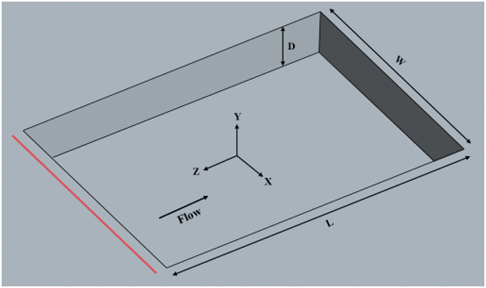
Figure 1: Model of the cavity region

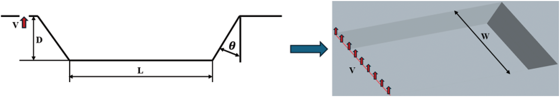
Figure 2: A cavity area model considering jet flow and front and rear wall inclination angles

3.2 Computational Domain and Boundary Conditions

In order to achieve a numerical simulation of the cavity that accurately reflects real-world conditions, it is imperative to establish a sufficiently large computational domain. Detailed specifications of this domain are illustrated in Fig. 3. The computational domain encompasses a width of 20 D and a height of 16 D. The distance from the leading edge of the cavity wall to the entrance of the computational domain is 12 D, while that from the trailing edge wall to the exit is 32 D. This extensive computational domain facilitates the full development of the turbulent wake within the cavity region, thereby enhancing the accuracy of the simulation. The cavity flow enters through the computational domain entrance, which is designated as a velocity inlet for the incoming air, set at a velocity of 111.11 m/s. The outlet of the computational domain serves as the wake outlet, configured as a pressure outlet with an initial surface pressure of 0. To conform to the requirements of the simulation, the side walls and the top surface of the computational domain are treated as symmetrical planes. Additionally, the bottom boundary is designated as a non-slip wall to closely approximate physical conditions. For the modeling of the jet slot, the jet slot surface is assigned as a velocity inlet without any further geometric modifications. This design choice is informed by the relevant research conducted by He [30], ensuring that the configuration effectively simulates the actual jet trajectory.

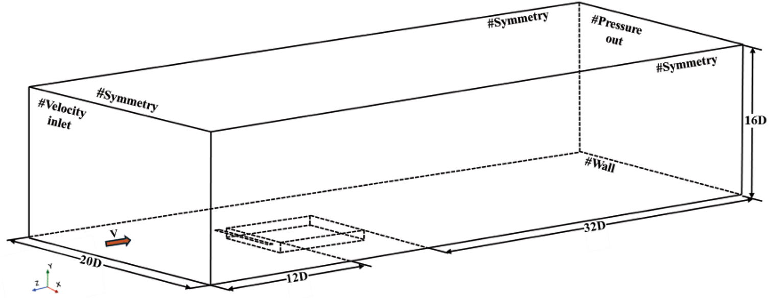
Figure 3: Computational domain and boundary conditions for the simulation

3.3 Mesh Strategy

This study uses a hybrid meshing approach that integrates prism layer meshes and trimmed volume meshes to ensure as much as possible the computational accuracy during numerical simulations, particularly in acoustic calculations. Considering the actual computational resources, the surface mesh size of the cavity is controlled at 1.5 mm, and the surface mesh size of the jet groove is controlled at 0.1 mm. Additionally, multiple refinement zones are introduced to selectively refine the mesh within the computational domain of the cavity. To accurately simulate the boundary layer flow between the incoming air and the cavity surface, a fine prismatic layer mesh consisting of 15 layers is generated on the cavity surface. The height of the first layer of this mesh is set to 0.01 mm, with a controlled mesh growth rate of 1.2. This meshing strategy results in approximately 9.3 million volume meshes within the cavity. The specific distribution of the grid around the cavity area is illustrated in Fig. 4.

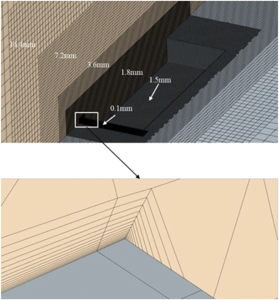
Figure 4: Mesh arrangement in the vicinity of the cavity area

3.4 Numerical Solution Setup

This article uses the commercial software Starccm+ to solve the model, with software version 17.06. In terms of numerical solution settings, the SIMPLE algorithm is used to solve the discrete flow control equations during numerical simulations. The convective terms in these equations are discretized using a second-order windward bounded center difference method. Conversely, the diffusion terms are solved directly employing a generalized second-order scheme. For gradient calculations within the numerical simulation, the mixed Gaussian method is applied. For time advancement, a second-order implicit unsteady state method is utilized, with a specified acoustic solution time step of 5 × 10−5 s. This configuration facilitates the analysis of aerodynamic noise generated within cavities at frequencies of up to 5000 Hz, ensuring both accuracy and stability of the resultant solutions. Before performing the acoustic simulation, a steady-state solution of the cavity region is obtained through 4000 iterations of RANS simulation, resulting in a converged steady-state flow field. Before solving acoustics, let the transient flow field in the cavity region develop to a certain extent. Following this, the transient flow field in the cavity region was allowed to evolve for a duration of 0.15 s before initiating the FW-H equation to compute and collect the aerodynamic noise present in the cavity area. The total duration for noise calculation and collection in the cavity was 0.21 s.

4  Verification of Calculation Methods and Mesh Strategies

Because of the restrictions in laboratory conditions, it is not feasible to confirm the accuracy of numerical simulations using wind tunnel tests. As a result, this study uses experimental data on open cavities from Plentovich et al. [31] to verify the meshing strategy and numerical methods applied in the current work. The geometric dimensions of the cavity model used for experimental verification are as follows: length L1 = 366 mm, width W1 = 244 mm, and depth D1 = 61 mm. Among them, L1/D1 = 6:1, W1/D1 = 4:1. The inflow velocity at the velocity inlet is 0.2 Mach, and the remaining boundary conditions are completely consistent with those in Section 3.2. The specific details are shown in Fig. 5.

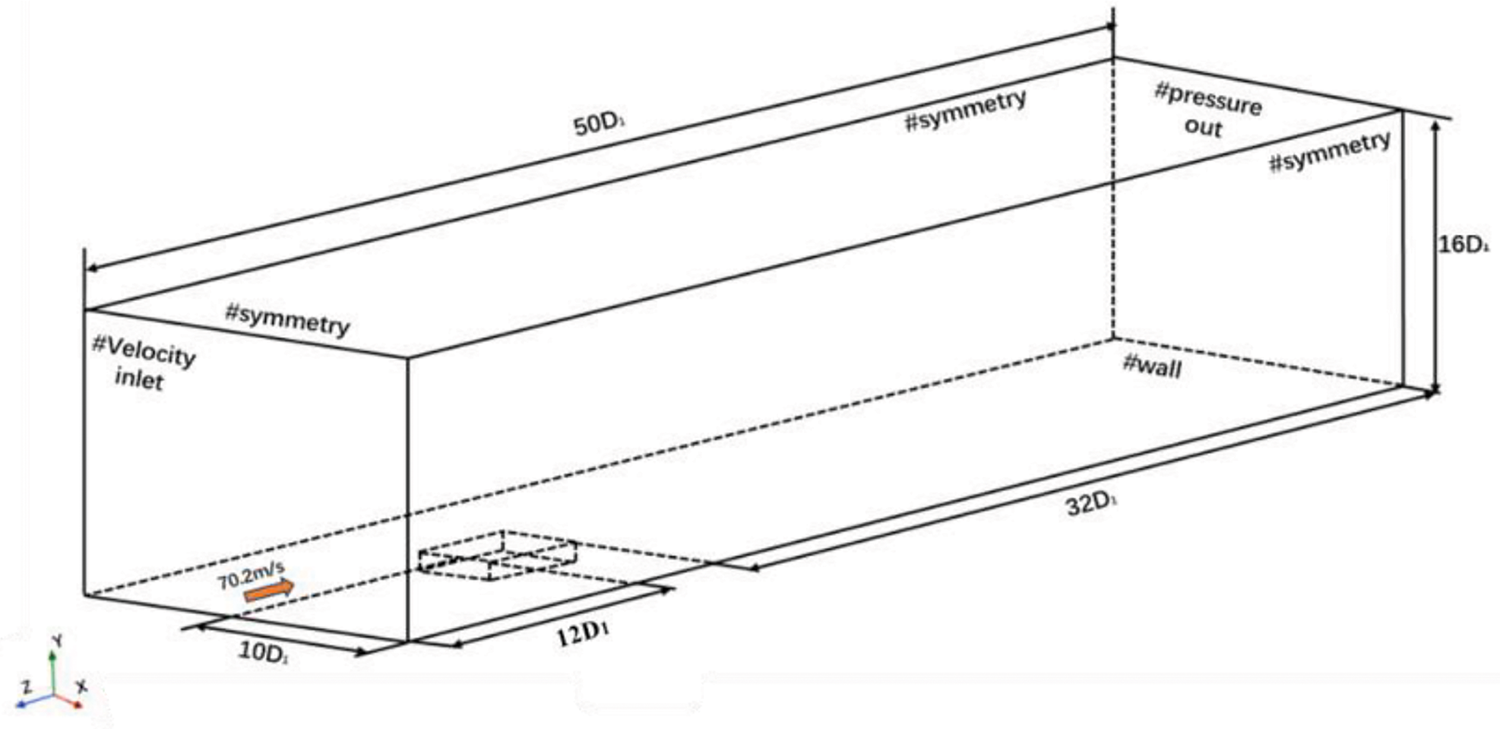
Figure 5: Geometric model settings for verification of cavity

To assess the impact of the meshing strategy on simulation outcomes, we systematically varied the surface mesh size of the clean cavities and the volume mesh size of the encrypted areas. Table 1 summarizes three distinct sets of meshing strategies, each corresponding to different mesh sizes. The resulting mesh volumes were quantified at 4.6 million, 6.3 million, and 8.2 million elements, respectively. The configuration of the refinement zone surrounding the cavity region is illustrated in Fig. 6.

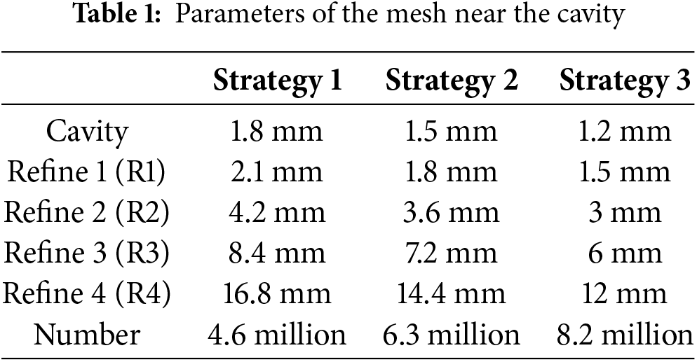
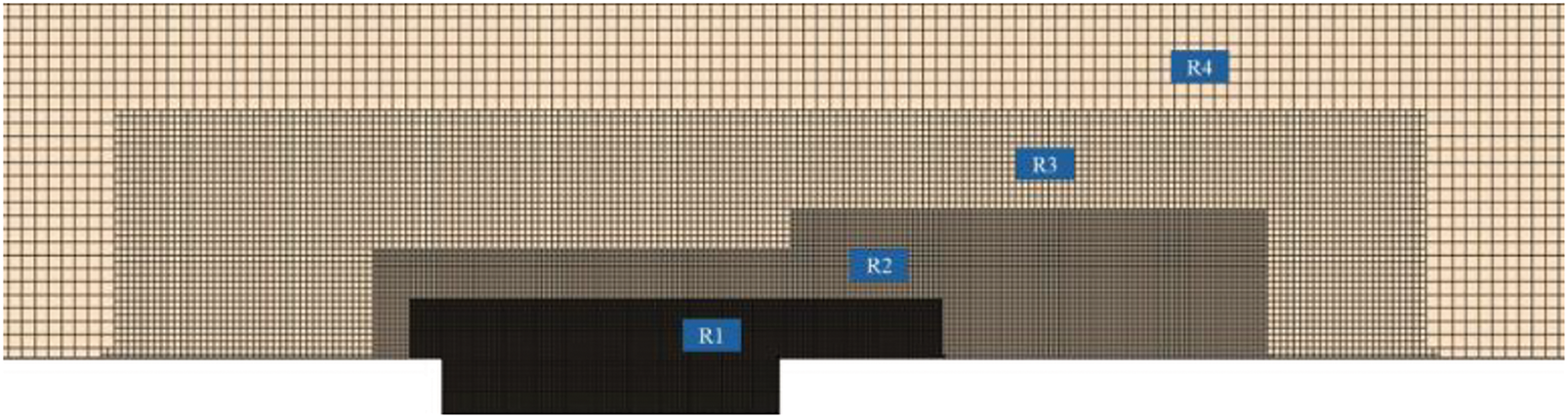
Figure 6: Arrangement of refinement zones for clean cavity meshes

This study utilizes experimental data from Plentovich et al. [31] on the pressure coefficient at the base of the cavity. It aims to assess and validate the grid strategy and numerical calculation methods employed in the referenced study. The definition of pressure coefficient CP is as follows:

CP=P−P∞1/2ρu∞2(5)

where p∞ represents the pressure at infinity, ρ denotes the fluid density, and u∞ is the free flow velocity.

The pressure coefficient is calculated by extracting pressure data from the centerline of the clean cavity bottom. Fig. 7 presents a comparative analysis of numerical simulation results and experimental data, where d/L1 represents the ratio of the measurement point to the cavity length. Analysis of this figure reveals that, in the front of the cavity area, although the calculation results exhibit fluctuations around the experimental data, there is almost no error between the two, and the development trend of the pressure coefficient is basically consistent. In the middle and rear of the cavity area, a notable degree of divergence is observed between the simulation and experimental results. Despite ongoing grid refinement leading to a marginal reduction in this discrepancy, the change remains insignificant. This inconsistency may be attributed to variations between the experimental conditions and those assumed in the numerical simulations conducted in this study, which encompasses factors such as temperature, air pressure, and other environmental parameters. Nevertheless, the overall distribution of the pressure coefficient at the cavity bottom in the simulation aligns well with the experimental outcomes, with differences falling within the acceptable range of experimental error. Therefore, the parameters and computational models applied to the cavity mesh in the pantograph area in the current study deemed appropriate, effectively balancing computational accuracy with resource utilization.

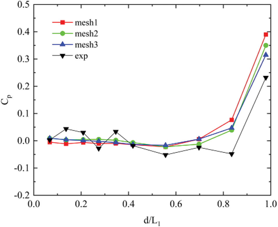
Figure 7: Pressure coefficient simulation and experimental results at the bottom of the cavity

5  Findings and Analysis

5.1 Sources of Noise

Fig. 8 illustrates the pressure pulsation amplitude on the cavity surface in the pantograph area, aiming to analyze how jet flow at varying velocities influences the intensity and distribution of dipole sources on the cavity surface in that region. The figure clearly shows that across all models, significant amplitude pulsations are evident at the bottom of the cavity and on the rear wall. However, when compared to the cavity model without jet (Base model), a clear trend emerges: in Jet 1 to Jet 4, as the jet velocity increases, the pressure pulsation amplitude on the bottom and rear walls of the cavity is significantly suppressed, while the pressure pulsation amplitude at the front of the cavity does not change significantly. This phenomenon indicates that the jet flow has a more significant impact on the rear of the cavity, while its impact on the front of the cavity is relatively small. The suppression of pressure pulsation amplitude in the rear and bottom areas becomes increasingly evident with higher jet velocities. However, the lack of significant alteration in the amplitude at the front indicates that the jet does not significantly affect pressure pulsations in that region. Based on the observed variations in pressure pulsation amplitude on the cavity surface, it can be inferred that the presence of the jet flow contributes to a reduction in aerodynamic noise in the cavity area. Moreover, this noise reduction effect appears to be more pronounced with increasing jet velocities. In the following sections, a detailed analysis of the flow field surrounding the cavity will be conducted to further substantiate this inference.

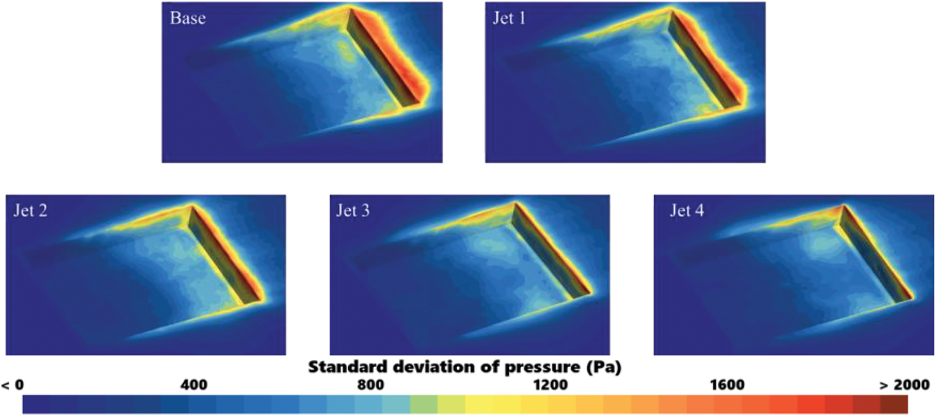
Figure 8: Pressure pulsation amplitude on the surface in the cavity region

5.2 Flow Field Analysis of Cavity Region

To better understand the impact of jets at varying speeds on pressure fluctuations within the cavity, this section will further examine how jets at different velocities affect the cavity flow field.

Fig. 9 illustrates the instantaneous vorticity in the vicinity of the cavity region. For the Base model, the incoming gas separates at the cavity’s leading edge. A part of the gas separates at the front of the cavity, and then moves toward the middle and rear of the cavity, where it generates a shedding vortex that interacts with both the rear portion of the cavity’s bottom surface and the trailing edge wall. As demonstrated in Fig. 7, significant pressure pulsations occur in the cavity bottom and the trailing edge wall of the Base model, which constitutes the primary cause of the aerodynamic noise generated in the cavity.

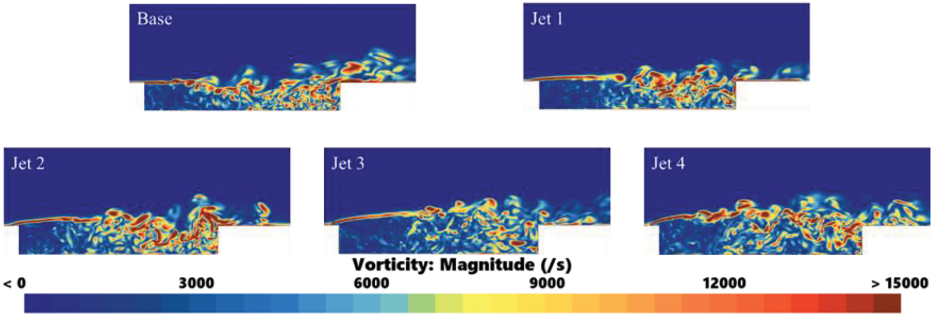
Figure 9: Instantaneous vorticity distribution around the cavity region

Models Jet 1 through Jet 4 exhibit a notable enhancement in the height of the shear layer and a reduction in flow separation at the leading edge of the cavity, as illustrated in Fig. 9. The results indicate that as jet velocity increases, the elevation of the shear layer also progresses upward. This dynamic leads to an expansion of the low-velocity region within the cavity. Furthermore, with the substantial reduction in flow separation at the front of the cavity, the incidence of shedding vortices entering the cavity is diminished, subsequently decreasing their interaction with the bottom and rear walls of the cavity. Corroborating this observation, the calculations presented in Fig. 8 indicate that the amplitude of pressure pulsations systematically decreases with increasing jet velocity.

The analysis presented in Fig. 9 indicates that the presence of a jet effectively reduces the interaction area between the shedding vortex and the rear wall of the cavity. However, Fig. 9 provides a snapshot of the vorticity distribution at a specific moment within the cavity region. To elucidate the dynamic process by which the jet mitigates the interaction area between the shedding vortex and the cavity back wall, Fig. 10 illustrates the temporal variations in vorticity for the Base model, Jet 2 model, and Jet 4 model over the designated time interval of 0−10Δt. From Fig. 10, it can be seen that vortices E1, E2, and E4 have all undergone processes of detachment, diffusion, and re-aggregation before ultimately colliding with the trailing edge wall of the cavity. As the jet velocity increases, the height of the vortex also increases, and the impact area between the vortex and the back wall of the cavity becomes smaller and smaller. Therefore, through the analysis of the variation of vorticity over time, it is more intuitively demonstrated that as the jet velocity increases, the impact area between the shedding vortex and the rear wall of the cavity gradually decreases, thereby reducing the surface pressure pulsation of the cavity. Supporting this observation, Fig. 8 indicates a decrease in pressure amplitude on the tail wall with increasing jet velocity. This reduction in pressure pulsation is likely to alleviate the aerodynamic noise generated in the cavity region, thereby signifying the efficacy of jet implementation in enhancing acoustic performance.

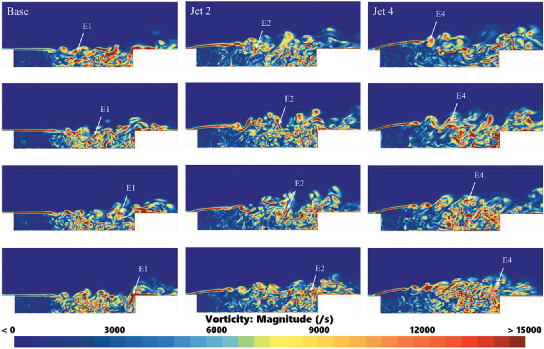
Figure 10: The variation of cavity vorticity distribution over time within the range of 0−10Δt

To gain a more intuitive understanding of the influence of the jet on the height of the shear layer above the cavity and the gas flow velocity inside the cavity, Fig. 11 presents the time-averaged streamlines for each cavity configuration. From the analysis of Figs. 9 and 10, when the shear layer interacts with the cavity’s rear wall, flow separation occurs once more. The separated gas moves toward the cavity’s bottom and then toward the front, creating a recirculation zone within the cavity that links the high-pressure region at the back with the low-pressure region at the front. Comparable flow separation and recirculation zones have been documented in previous studies, such as reference [29].

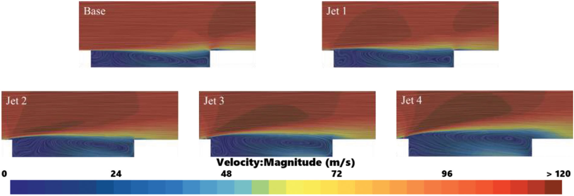
Figure 11: Time averaged streamlines and velocity cloud clouds around the cavity area

Upon the introduction of the jet, a comparison with the Base model indicates that in the Jet 1 through Jet 4 models, an increase in jet velocity correlates with a rise in the shear layer height above the cavity. The center of the recirculation zone within the cavity progressively shifts toward the rear. Coupling this observation with prior vorticity analyses allows us to infer that as jet velocity escalates, the height of the shear layer similarly increases, resulting in a reduced number of shedding vortices impacting the cavity’s rear wall. Consequently, following flow separation at the rear wall, the vorticity directed toward the front of the cavity diminishes, prompting the recirculation zone’s center to migrate rearward. The decrease in the frequency of shedding vortices striking the rear wall is also associated with a reduction in the amplitude of pressure pulsations present on the back wall, as vividly demonstrated in Fig. 8.

In terms of turbulent kinetic energy, the presence of jets leads to a significant increase in turbulent kinetic energy above the cavity region compared to the Base model without jets. The details are shown in Fig. 12. As the velocity of the jet increases, the height of the lifted shear layer also rises, resulting in a gradual increment in the amplitude of turbulent kinetic energy above the cavity. This occurs because the jet introduction elevates the shear layer height, which subsequently increases the velocity of the incoming air within the shear layer. Specifically, with higher jet velocities, the shear layer attains greater heights, consequently leading to an increased magnitude of turbulent kinetic energy. Although the presence of a jet increases the turbulent kinetic energy amplitude above the cavity, we can clearly see from Fig. 12 that compared to the cavity model without a jet (Base model), the turbulent kinetic energy amplitude at the bottom and rear wall of the cavity gradually decreases with escalating jet velocities. Furthermore, as jet velocity continues to increase, the region of low turbulent kinetic energy within the cavity expands. This expansion is attributable to the elevated height of the shear layer, which subsequently reduces the influx of high-velocity airflow into the cavity, resulting in a decrease in the shedding vortices. Consequently, this process fosters the growth of low-velocity regions within the cavity, thereby broadening the area characterized by low turbulent kinetic energy. When analyzed in conjunction with Fig. 7, it becomes evident that the lower amplitude of turbulent energy correlates with a diminished amplitude of surface pressure pulsations. In turn, reduced surface pressure pulsation amplitude is associated with lower noise levels.

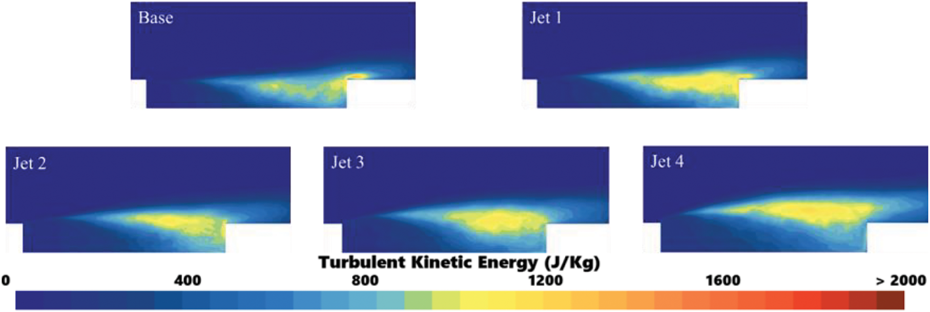
Figure 12: Turbulent kinetic energy distribution of wake in cavity region

Based on the previous analysis of the flow field, it is evident that increased jet velocity correlates with reduced surface pressure pulsations within the cavity. However, even in the Jet 4 model, which exhibits the highest jet velocity, significant pressure fluctuations persist at the junction of the rear cavity and the trailing edge wall. The Jet 5 model addresses this issue effectively by incorporating inclination angles for the front and rear walls, as illustrated in the results presented in Fig. 13.

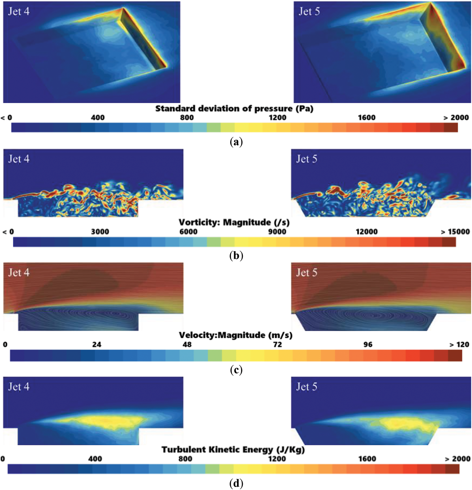
Figure 13: Related flow field results of Jet 5 model. (a) Surface pressure pulsation; (b) Instantaneous vorticity distribution; (c) Time-averaged streamlines as well as velocity clouds; (d) Turbulent kinetic energy distribution

As shown in Fig. 13a, following the implementation of inclination angles in the Jet 5 model, surface pressure pulsations at the junction of the bottom and rear walls within the cavity are notably diminished compared to the Jet 4 model. According to Fig. 13b, in both the Jet 4 and Jet 5 models, the vortex structure generated by the jet undergoes detachment, diffusion, and reaggregation, which aligns with the analysis presented in Section 5.2. Notably, the elevation of the shear layer in both models remains comparable, attributable to the constant jet velocity. Nevertheless, the vorticity distribution at the cavity’s rear and along the trailing edge wall is altered due to the introduction of the inclination angle. As discussed in Section 5.2, the shedding vortex experiences flow separation after interacting with the rear wall of the cavity, causing a portion of the airflow to travel along the rear wall towards the bottom of the cavity. The inclination angle in the Jet 5 model induces a buffering effect on the vorticity directed towards the cavity’s bottom, resulting in reduced vorticity accumulation at the junction of the rear and trailing edge walls when compared to the Jet 4 model. Furthermore, the inclination angle prevents the post-flow separation vortex structure from directly contacting the cavity’s bottom, contributing to a significant reduction in surface pressure pulsations at the junction of the rear and trailing edge walls in the Jet 5 model. Based on Fig. 13c, the recirculation area in the Jet 4 model is more flattened near the rear wall of the cavity compared to the Jet 5 model, suggesting that the interaction between its vortex structure and the rear and side walls of the cavity is more intense. Additionally, as depicted in Fig. 13d, the presence of the jet results in high-amplitude turbulent kinetic energy forming above the cavity. However, at the junction of the rear and trailing edge walls in the cavity, the turbulent kinetic energy amplitude in the Jet 5 model is significantly lower than in the Jet 4 model, which also indirectly supports the previous analysis.

To have a more intuitive understanding of the variations in pressure pulsation values occurring on the cavity surface, it is necessary to quantitatively analyze the amplitude of pressure pulsation on the bottom of the cavity. Consequently, pressure pulsation data must be extracted from this region, with the specific extraction locations delineated in Fig. 14. In this depiction, Line 1 is the centerline of the cavity bottom, and Line 2 is parallel to Line 1, with a distance of 0.13 m between them. Line 3 and Line 2 are symmetrical about Line 1.

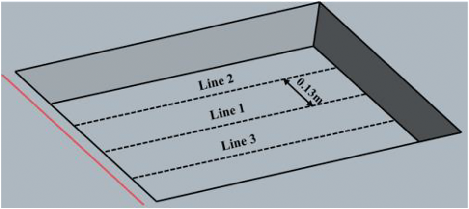
Figure 14: Schematic diagram of data extraction location for pressure pulsation amplitude

Fig. 15 illustrates the amplitude of surface pressure fluctuations at the bottom of each model cavity. From Fig. 14, we can clearly see that as the jet velocity increases, the surface pressure fluctuation data at the bottom of the cavity gradually decreases, which is consistent with the previous analysis. Specifically, at the rear of the cavity (0.8 L-L), the Jet model that incorporates jet flow shows a marked reduction in surface pressure amplitude when compared to the Base model, which omits jet flow. Notably, the Jet 4 model demonstrates significant pressure fluctuation amplitude at the interface of the cavity bottom and the rear wall (L2/L = 1). However, this issue is effectively mitigated in the Jet 5 model, which incorporates an inclination angle for both the front and rear walls. This design modification leads to a reduction in pressure pulsation amplitude at the junction of the cavity bottom and the rear wall. Consequently, it can be postulated that the aerodynamic noise produced by the Jet 5 model is the lowest among all tested models.

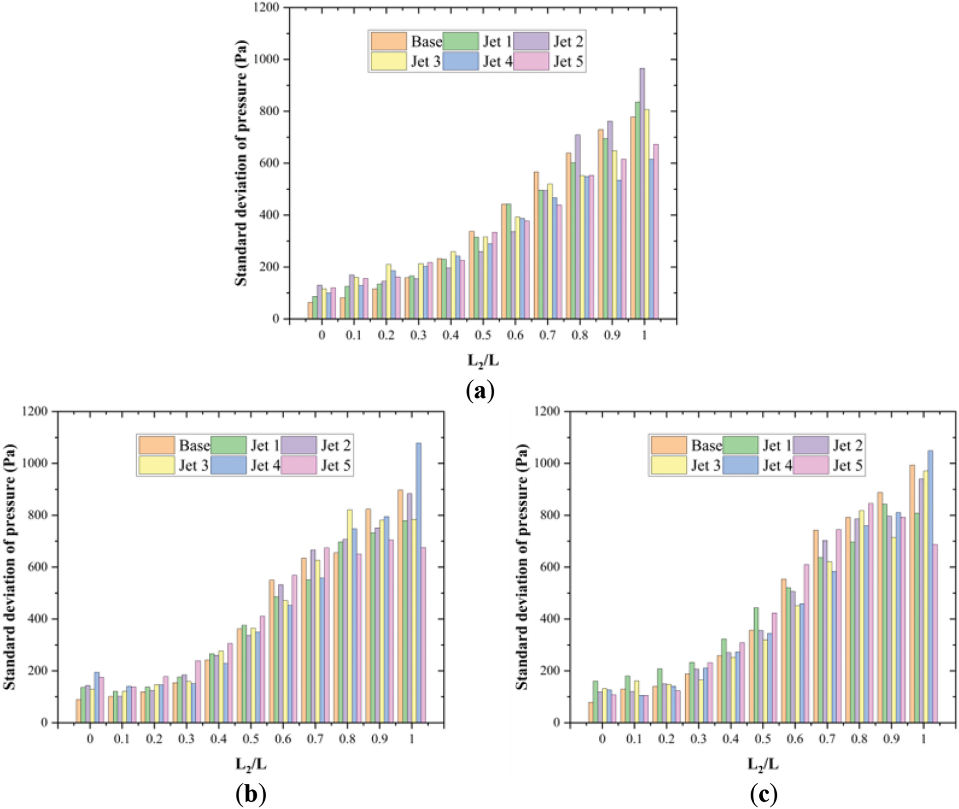
Figure 15: Amplitude of pressure pulsation at the bottom of the cavity at different positions. (a) Line 1; (b) Line 2; (c) Line 3

In summary, the introduction of the jet elevates the shear layer and thus results in an increased inflow velocity within the upper shear layer of the cavity. This phenomenon simultaneously enlarges the shielding area inside the cavity, leading to a decrease in the flow velocity within the cavity itself. As the shear layer is raised higher due to the jet action, the shedding vortex structures generated by the incoming airflow encounter a reduced surface area upon collision with the rear wall of the cavity, which leads to a decrease in the extent of flow separation subsequent to these interactions. Consequently, the amplitude of surface pressure pulsations on the bottom and rear wall surfaces of the cavity diminishes progressively with increasing jet velocity. Furthermore, the relationship between jet velocity and the reduction of pressure pulsations on the cavity surface becomes increasingly pronounced at higher jet velocities. Specifically, within the velocity range of 111.11 m/s, it can be concluded that enhanced jet velocities correlate with diminished surface pressure pulsations within the cavity, which may subsequently lead to a reduction in aerodynamic noise levels. However, although the surface pressure pulsation amplitude of the Jet 4 model is already very small, a large pressure pulsation amplitude still appears at the junction of the cavity bottom and the rear wall. At this point, modifying the front and rear walls of the cavity can provide a buffering effect on the interaction between the vortex structure and the bottom of the cavity. Therefore, compared with the Jet 4 model, the Jet 5 model further reduces the pressure pulsation amplitude on the cavity surface. The smaller the amplitude of surface pressure pulsation, the smaller the noise generated.

5.3 Far-Field Noise Generated in the Cavity Area

To investigate the aerodynamic noise generated in the cavity region, nine acoustic measurement points were placed at various locations above and along the sides of the cavity, as illustrated in Fig. 16. The entire cavity is treated as a discrete noise source for acoustic analysis. The sound magnitude is evaluated based on the sound pressure level, defined by the following equation:

SPL=20log⁡(P/P0)dB(6)

where SPL represents the sound pressure level, P represents the sound pressure, and P0 represents the reference sound pressure.

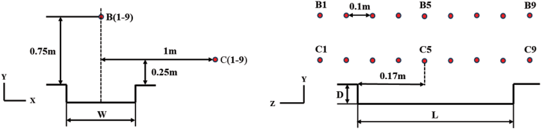
Figure 16: Distribution of acoustic measurement point positions

Fig. 17 illustrates the noise reduction achieved by the Jet 1 to Jet 5 models in comparison to the Base model. The figure clearly shows that for the Jet 1 to Jet 4 models, which only introduce jets, the noise reduction within the cavity improves progressively with an increase in jet velocity. The Jet 4 model demonstrates the most significant reduction, achieving approximately 4 dB. In contrast, the Jet 5 model further enhances aerodynamic noise reduction, yielding a maximum decrease of approximately 6 dB compared to the Jet 4 model. Building on the previous flow field analysis, the combination of the jet and the inclination angles of the front and rear walls reduces the interaction between the shedding vortices and the rear walls of the cavity, effectively achieving the goal of reducing aerodynamic noise within the cavity. To further understand the corresponding noise reduction mechanism, the spectral results of Jet 4 and Jet 5 models at B8 and C8 are presented, as shown in Fig. 18. Additionally, Fig. 19a evaluates the sound pressure levels of each model at these measurement points, while Fig. 19b provides the one-third octave band data for the Jet 5 model at B8 and C8, further emphasizing its noise reduction efficacy. As seen in Fig. 18, the spectral results for the cavity at both B8 and C8 display a broadband characteristic, with predominant noise occurring in the 500 Hz range. The peak of vortex shedding is clear in the spectrum, dominating the overall noise, with frequencies primarily concentrated between 200 and 500 Hz [27,29]. Fig. 18a,b demonstrates a substantial reduction in the peak value of the shedding vortex following the introduction of jets in the Jet 4 model, with further attenuation observed in the Jet 5 model as a result of incorporating the inclined front and rear walls.

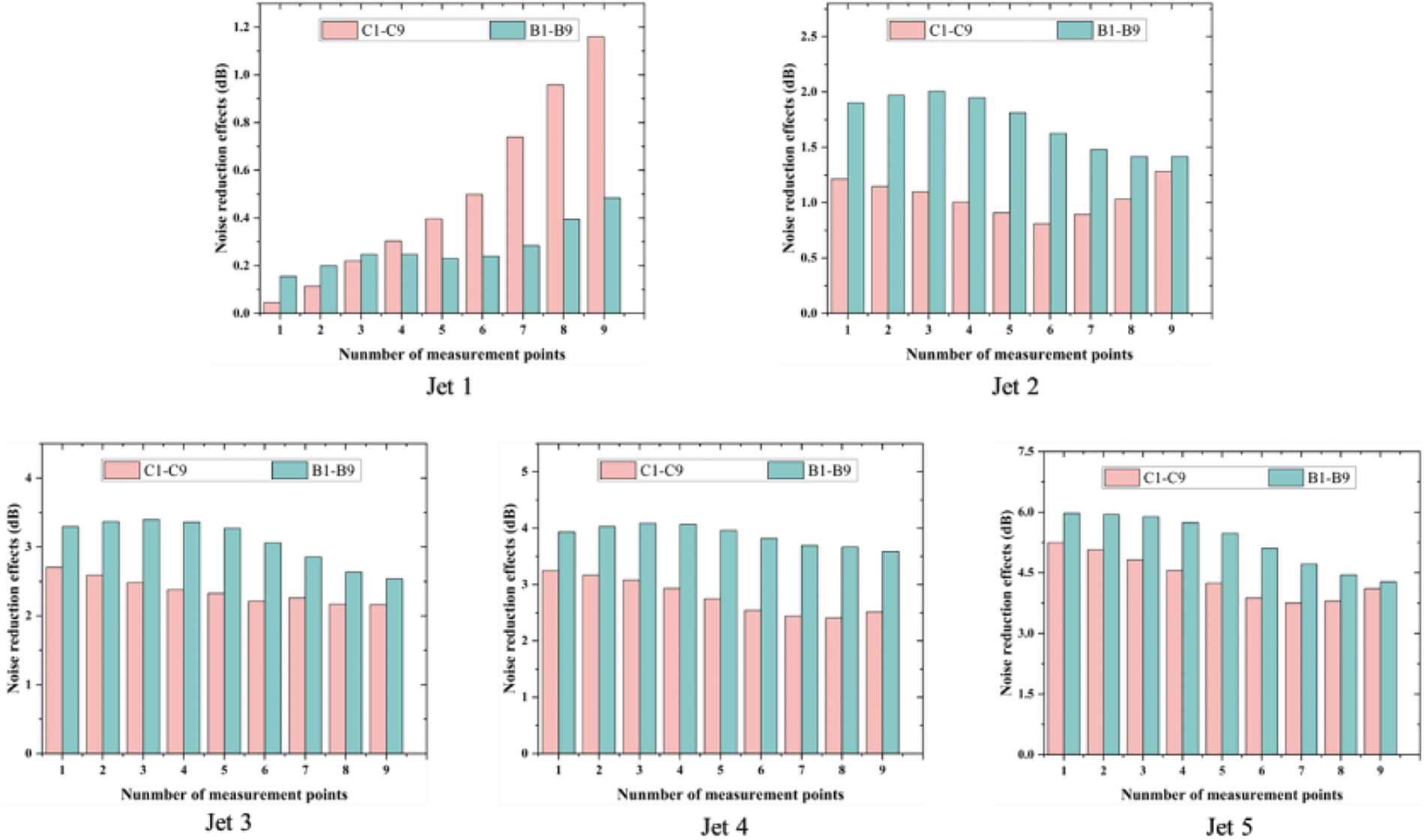
Figure 17: Noise reduction effect of each model (compared to the base model)

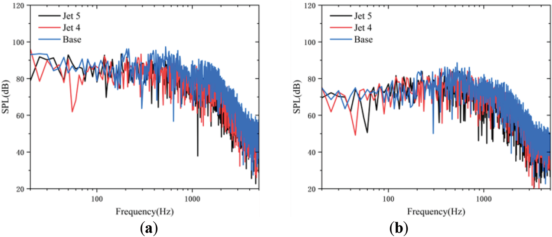
Figure 18: Spectral data at B8 and C8. (a) Spectral results at point B8; (b) Spectral results at point C8

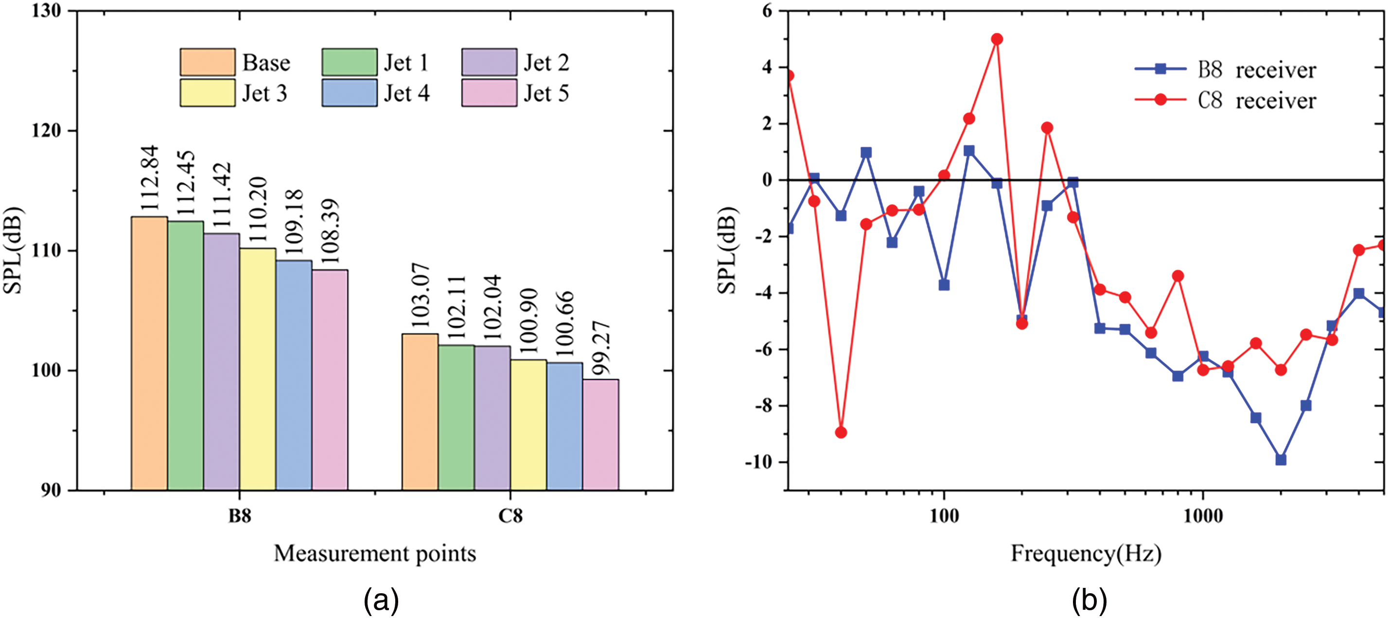
Figure 19: Overall sound pressure level result and one-third frequency spectra result. (a) Overall sound pressure level result; (b) The one-third octave band result of Jet 5

It is important to note that, while increasing jet velocity results in higher noise levels from the jet slot, the impact on overall cavity noise must be considered. According to findings from references [25,32], at a velocity of 400 km/h, the noise generated by the jet itself has no significant adverse effect on the noise reduction outcomes. Consequently, the observed noise reduction in cavity aerodynamic noise is deemed reliable.

6  Conclusion

This study employs the IDDES method coupled with the FW-H equation to investigate the effects of varying jet velocities and modifications of the front and rear walls on the aerodynamic noise generated by high-speed train pantograph chambers. The primary conclusions drawn from this research are as follows:

1.    Numerical simulations of the flow field reveal that the introduction of a jet significantly mitigates flow separation occurring at the front of the cavity. The presence of the jet alters the characteristics of the shear layer; specifically, as jet velocity increases, the elevation of the shear layer also increases. Consequently, the interaction area between the shedding vortices and the rear wall of the cavity diminishes. The intensity of the dipole source (surface pressure pulsation) at the rear of the cavity decreases progressively, reaching its minimum value in the Jet 4 model.

2.    For the Jet 5 model, additional modifications in the form of inclined angles at the front and rear walls are implemented based on the findings of the Jet 4 model. Analysis indicates that the detached vortex experiences a secondary airflow separation upon colliding with the rear wall of the cavity. Due to the introduced inclination angles, the separated airflow is prevented from directly interacting with the bottom of the cavity. This design further weakens the dipole source strength at the junction between the cavity bottom and the trailing edge wall.

3.    From an acoustical perspective, the aerodynamic noise associated with the cavity model enhanced by the jet shows considerable improvement. The sound pressure level of the aerodynamic noise in the Jet 4 model is reduced by approximately 4 dB. Further analysis indicates that, compared to the Jet 4 model, the Jet 5 model exhibits continued optimization of aerodynamic noise, achieving a maximum reduction of 6 dB and displaying markedly improved noise reduction characteristics.

In summary, the introduction of a jet helps delay flow separation at the front edge of the cavity and elevates the shear layer, which reduces the interaction area between the shedding vortices above the cavity and the rear wall, thereby lowering the aerodynamic noise produced by the cavity. Additionally, by modifying the angles of the cavity’s front and rear walls in conjunction with the jet, it is possible to further diminish the amplitude of surface pressure pulsations at the cavity’s base and at the junction with the rear wall, thereby contributing to additional noise reduction. However, the current findings presented in this study primarily evaluate the aerodynamic noise characteristics of the cavity based only on jet velocity and a singular inclination angle. For practical engineering applications, the depth of this analysis remains insufficient. Consequently, it is imperative to further investigate the optimal positioning and flow rate of the jet, as well as the inclination angles of the front and rear walls of the cavity. Future research will focus on these critical aspects.

Acknowledgement: None.

Funding Statement: This work was supported by National Natural Science Foundation of China (12172308).

Author Contributions: Yangyang Cao: Conceptualization, Methodology, Data curation, Formal analysis, Writing original draft. Jiye Zhang: Funding acquisition, Supervision. Jiawei Shi: Writing review & editing, Supervision. Yao Zhang: Editing, Supervision. All authors reviewed the results and approved the final version of the manuscript.

Availability of Data and Materials: The datasets generated and analyzed during the current study are available from the corresponding author on reasonable request.

Ethics Approval: Not applicable.

Conflicts of Interest: The authors declare no conflicts of interest to report regarding the present study.

References

1. Uda T, Akutsu M. Sound source distribution of high-speed trains and reduction of aerodynamic bogie noise. In: INTER-NOISE and NOISE-CON Congress and Conference Proceedings; 2023 May 15–18; Grand Rapids, MI, USA. Edgewater Pl. Wakefield, MA, USA: Institute of Noise Control Engineering; 2023. p. 3709–16. [Google Scholar]

2. AbdelGawad AF, Aljameel NM, Shaltout RE. Computational modelling of the aerodynamic noise of the full-scale pantograph of high-speed trains. J Adv Res Fluid Mech Therm Sci. 2022;93(1):94–109. doi:10.37934/arfmts.93.1.94109. [Google Scholar] [CrossRef]

3. Iglesias EL, Thompson D, Paniagua JM, García JG. On the feasibility of a component-based approach to predict aerodynamic noise from high-speed train bogies. Appl Acoust. 2023;211:109536. doi:10.1016/j.apacoust.2023.109536. [Google Scholar] [CrossRef]

4. Noh HM, Choi S, Hong S, Kim SW. Investigation of noise sources in high-speed trains. Proc Inst Mech Eng Part F: J Rail Rapid Transit. 2014;228(3):307–22. doi:10.1177/0954409712473095. [Google Scholar] [CrossRef]

5. Zhang J, Guo T, Sun B, Zhou S, Zhao W. Research on characteristics of aerodynamic noise source for high-speed train. J China Railw Soc. 2015;37(6):10–8. doi:10.3969/j.issn.1001-8360.2015.06.002. [Google Scholar] [CrossRef]

6. Shaltout RE, Aljameel NM, AbdelGawad AF. Modeling and simulation of the aerodynamic noise of high-speed train’s pantograph. J Eng. 2022;2022(1):1164017. doi:10.1155/2022/1164017. [Google Scholar] [CrossRef]

7. Thompson DJ, Latorre Iglesias E, Liu X, Zhu J, Hu Z. Recent developments in the prediction and control of aerodynamic noise from high-speed trains. Int J Rail Transp. 2015;3(3):119–50. doi:10.1080/23248378.2015.1052996. [Google Scholar] [CrossRef]

8. Suzuki M, Okura N, Murao T, Baranwal A. Aerodynamic noise reduction of pantograph head by small rods. J Fluid Flow Heat Mass Transf. 2024;11(1):64. doi:10.11159/jffhmt.2024.007. [Google Scholar] [CrossRef]

9. Saito M, Mizushima F, Wakabayashi Y, Kurita T, Nakajima S, Hirasawa T. Development of new low-noise pantograph for high-speed trains. In: Noise and Vibration Mitigation for Rail Transportation Systems: Proceedings of the 13th International Workshop on Railway Noise; 2019 Sep 16–20; Ghent, Belgium. Berlin/Heidelberg, Germany: Springer International Publishing; 2021. p. 81–9. [Google Scholar]

10. Yuan X, Yuan D, Tang L, Wang X. Study on active and passive cooperative noise reduction of high-speed train’s pantograph based on fluent. Intell Comput Appl. 2021;11(2):149–54. doi:10.47176/jafm.17.7.2472. [Google Scholar] [CrossRef]

11. Kim H, Hu Z, Thompson D. Effect of different typical high speed train pantograph recess configurations on aerodynamic noise. Proc Inst Mech Eng Part F J Rail Rapid Transit. 2021;235(5):573–85. doi:10.1177/0954409720947516. [Google Scholar] [CrossRef]

12. Tan XM, Yang ZG, Tan XM, Wu XL, Zhang J. Vortex structures and aeroacoustic performance of the flow field of the pantograph. J Sound Vib. 2018;432:17–32. doi:10.1016/j.jsv.2018.06.025. [Google Scholar] [CrossRef]

13. Yu PX, Bai JQ, Guo BZ, Han X, Han SS. Suppression of aerodynamic noise by altering the form of shear layer in open cavity. J Vib Shock. 2015;34(1):156–64. doi:10.1186/s42774-022-00119-9. [Google Scholar] [CrossRef]

14. Saddington AJ, Thangamani V, Knowles K. Comparison of passive flow control methods for a cavity in transonic flow. J Aircr. 2016;53(5):1439–47. doi:10.2514/1.C033365. [Google Scholar] [CrossRef]

15. Araddag S, Gelisli KA, Yalddir EC. Effects of active and passive control techniques on Mach 1.5 cavity flow dynamics. Int J Aerosp Eng. 2017;2017(1):8253264. doi:10.1155/2017/8253264. [Google Scholar] [CrossRef]

16. Kim H. Unsteady aerodynamics of high speed train pantograph cavity flow control for noise reduction. In: 22nd AIAA/CEAS Aeroacoustics Conference; 2016 May 30–Jun 1; Lyon, France. 2848 p. [Google Scholar]

17. Kim H, Hu Z, Thompson D. Effect of cavity flow control on high-speed train pantograph and roof aerodynamic noise. Railw Eng Sci. 2020;28:54–74. doi:10.1007/s40534-020-00205-y. [Google Scholar] [CrossRef]

18. Yu PX, Bai JQ, Guo BZ, Han X, Han SS. Suppression effect of jet flow on aerodynamic noise of 3D cavity. Appl Mech Mater. 2014;444:588–95. doi:10.4028/www.scientific.net/AMM.444-445.588. [Google Scholar] [CrossRef]

19. Zhang Z, Miao X, Liu D, Song R, Yuan T, Yang J. Cavity noise reduction of a high-speed train pantograph through jet parameter optimization. Proc Inst Mech Eng Part F J Rail Rapid Transit. 2024;7(17):13998–1410. doi:10.1177/09544097241251912. [Google Scholar] [CrossRef]

20. Ukai T, Zare-Behtash H, Erdem E, Lo KH, Kontis K, Obayashi S. Effectiveness of jet location on mixing characteristics inside a cavity in supersonic flow. Exp Therm Fluid Sci. 2014;52:59–67. doi:10.1016/j.expthermflusci.2013.08.022. [Google Scholar] [CrossRef]

21. Spalart PR, Deck S, Shur ML, Squires KD, Strelets MK, Travin A. A new version of detached-eddy simulation, resistant to ambiguous grid densities. Theor Comput Fluid Dyn. 2006;20:181–95. doi:10.1007/s00162-006-0015-0. [Google Scholar] [CrossRef]

22. Shur ML, Spalart PR, Strelets MK, Travin AK. A hybrid RANS-LES approach with delayed-DES and wall-modelled LES capabilities. Int J Heat Fluid Flow. 2008;29(6):1638–49. doi:10.1016/j.ijheatfluidflow.2008.07.001. [Google Scholar] [CrossRef]

23. Squires K, Forsythe J, Morton S, Strang W, Wurtzler K, Tomaro R et al. Progress on detached-eddy simulation of massively separated flows. In: 40th AIAA Aerospace Sciences Meeting & Exhibit; 2002 Jan 14–17; Reno, NV, USA. 1021 p. [Google Scholar]

24. Williams JF, Hawkings DL. Sound generation by turbulence and surfaces in arbitrary motion. Philos Trans R Soc Lond Ser A Math Phys Sci. 1969;264(1151):321–42. doi:10.1098/rsta.1969.0031. [Google Scholar] [CrossRef]

25. Cao Y, Zhang J, Shi J, Ma Y. The influence of jet on aerodynamic noise in the pantograph area at different sinking heights. Phys Scr. 2024;99(10):105228. doi:10.1088/1402-4896/ad7413. [Google Scholar] [CrossRef]

26. Zhu JY, Hu ZW, Thompson DJ. Flow simulation and aerodynamic noise prediction for a high-speed train wheelset. Int J Aeroacoust. 2014;13(7–8):533–52. doi:10.1260/1475-472X.13.7-8.533. [Google Scholar] [CrossRef]

27. Zhao YY, Yang ZG, Li QL, Xia C. Analysis of the near-field and far-field sound pressure generated by high-speed trains pantograph system. Appl Acoust. 2020;169:107506. doi:10.1016/j.apacoust.2020.107506. [Google Scholar] [CrossRef]

28. Farassat F. Derivation of formulations 1 and 1A of farassat. Hanover, MD, USA: NASA Center for AeroSpace Information (CASI); 2007. [Google Scholar]

29. Yang DG, Li JQ, Fan ZL, Luo XF, Liang JM. Investigation on aerodynamic noise characteristics of cavity flow at high subsonic speeds. Acta Aerodyn Sin. 2010;28(6):703–7. [Google Scholar]

30. He Y. Aerodynamic noise simulation of high-speed train bogie [dissertation]. Southampton, UK: University of Southampton; 2023. [Google Scholar]

31. Plentovich EB, Stallings RL Jr, Tracy MB. Experimental cavity pressure measurements at subsonic and transonic speeds. Washington, DC, USA: National Aeronautics and Space Administration; 1993. [Google Scholar]

32. Shi J, Zhang J, Li T. Aerodynamic noise reduction of high-speed pantograph by introducing planar jet on leeward surface of panhead. J Wind Eng Ind Aerodyn. 2024;250:105780. doi:10.1016/j.jweia.2024.105780. [Google Scholar] [CrossRef]