
 Submit a Paper
 Propose a Special lssue
 Open Access
ARTICLE

Numerical Investigation of Stress and Toughness Contrast Effects on the Vertical Propagation of Fluid-Driven Fractures in Shale Reservoirs
State Key Laboratory of Oil & Gas Reservoir Geology and Exploitation, Southwest Petroleum University, Chengdu, 610500, China
* Corresponding Author: Manqing Qian. Email:
(This article belongs to the Special Issue: Fluid and Thermal Dynamics in the Development of Unconventional Resources II)
Fluid Dynamics & Materials Processing 2025, 21(6), 1353-1377. https://doi.org/10.32604/fdmp.2025.061652
Received 29 November 2024; Accepted 13 March 2025; Issue published 30 June 2025
 View Full Text
 Download PDF
Abstract
Shale reservoirs are characterized by numerous geological discontinuities, such as bedding planes, and exhibit pronounced heterogeneity across rock layers separated by these planes. Bedding planes often possess distinct mechanical properties compared to the surrounding rock matrix, particularly in terms of damage and fracture behavior. Consequently, vertical propagation of hydraulic fractures is influenced by both bedding planes and the heterogeneity. In this study, a numerical investigation into the height growth of hydraulic fractures was conducted using the finite element method, incorporating zero-thickness cohesive elements. The analysis explored the effects of bedding planes, toughness contrasts between layers, and variations in in-situ stress across different strata. The results reveal that hydraulic fractures are more likely to propagate along bedding planes instead of traversing them and extending vertically into barrier layers when (1) bedding strength is low, (2) stress contrast between layers is high, and (3) toughness contrast is significant. Furthermore, for a given bedding strength, increased stress contrast or higher toughness contrast between layers elevate hydraulic fracture extension pressure. When a substantial stress difference exists between layers (Lc = 0.4), hydraulic fractures preferentially propagate along bedding planes. Conversely, as bedding strength increases, the propagation distance along bedding planes decreases, accompanied by an amplified horizontal compressive stress field. Notably, when the stress difference is sufficiently small (SD < −0.2), a phenomenon termed “stress rolling” emerges, wherein hydraulic fractures deviate from vertical growth and instead extend along a near-horizontal trajectory.Keywords
Shale reservoirs, typically deeply buried, exhibit low porosity and permeability due to their compact pore structure. These inherent properties necessitate advanced stimulation techniques to enable efficient hydrocarbon extraction. Among these, hydraulic fracturing plays a critical role by generating artificial fracture networks to enhance reservoir productivity.
Controlling hydraulic fracture height remains crucial for ensuring successful fracturing operations. Inaccurate fracture height predictions may compromise optimized fracturing designs, potentially causing fluid and proppant migration into non-productive zones or aquifer penetration, which risks undesired fluid influx. For decades, researchers have widely recognized the stress contrast between geological layers as the primary factor influencing hydraulic fracture height growth. However, models relying solely on stress contrast tend to overpredict fracture heights compared with field observations [1–3]. This discrepancy is attributed to the neglect of the influence of geological discontinuities (e.g., bedding planes) in existing models. These structural features exhibit distinct mechanical properties, such as fracture toughness, that significantly differ from those of the intact rock matrix. Consequently, bedding planes can disturb hydraulic fracture propagation [4].
The effectiveness of bedding planes in restricting fracture height growth primarily depends on their intrinsic properties, including interfacial strength, dip angle, and bedding plane density (defined as the number of planes per unit interval). Early laboratory experiments showed that uncemented or weakly cemented bedding planes typically arrest hydraulic fracture propagation [5]. Through combined theoretical and experimental analyses, Daneshy identified the strength of bedding planes between adjacent layers as a key factor in influencing fracture height growth. When interfacial bonding between layers is strong, fractures are difficult to contain within the reservoir, whereas weak interfaces effectively limit fracture height [6]. Xu et al. examined the role of interface density in fracture containment. Their results indicated that a single interface acts as a toughness or stiffness barrier, while multiple closely spaced interfaces collectively form a stress barrier. The effectiveness of interfaces to constrain fracture height improves with increased bedding plane density [7]. Huang et al. employed the Cohesive Zone Method (CZM) to analyze the impact of dip angle on hydraulic fracture propagation in coal-rock formations. Their findings indicated that at dip angles of 0° and 15°, hydraulic fractures (HFs) propagate along the maximum horizontal principal stress direction without substantial branching. At dip angles of 30° and 45°, HFs penetrate the bedding plane, generating branched networks with significant shear slip. As dip angles increase to 60° and 75°, HFs become confined between bedding layers [8].
Variations in rock mechanical properties, such as elastic modulus, fracture toughness, and in-situ stress conditions, significantly affect fracture propagation patterns in stratified formations. Gudmundsson and Brenner demonstrated that rock layers with elastic moduli 10–100 times lower than adjacent formations absorb most tensile stresses at fracture tips [9]. This stress absorption impedes vertical fracture expansion and forms T-shaped fractures, as shown in Fig. 1. Jeffrey and Bunger further emphasized that stiffness contrasts across interfaces create stress differences, effectively acting as barriers to vertical fracture growth [10]. Huang et al. investigated the effects of stiffness, toughness, and stress contrasts between layers, particularly under interfacial slip conditions. Huang’s findings indicated that the elastic modulus ratio between adjacent layers primarily governs how hydraulic fractures approach interfaces. After the fracture reaches an interface, its further propagation is primarily controlled by the toughness contrast. If the fracture penetrates the interface, the stress contrast then becomes the dominant factor controlling vertical growth [11].
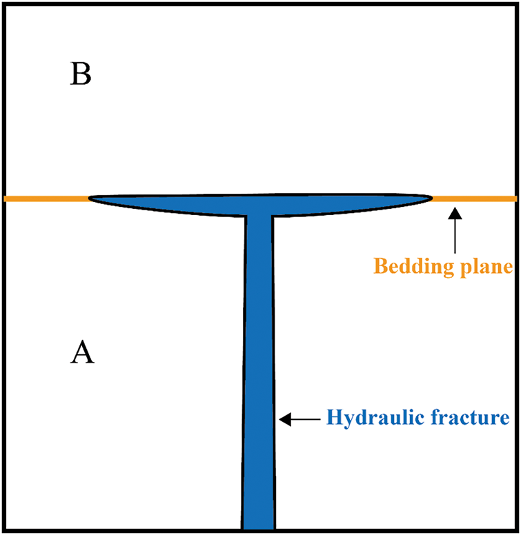
Figure 1: The T-shaped growth of hydraulic fractures
Previous studies have demonstrated that rock mechanical properties and bedding planes significantly influence fracture propagation in shale reservoirs. However, fracture height growth is influenced by multiple factors. A thorough analysis of reservoir stress state, material properties, and structural characteristics is necessary to improve prediction accuracy and optimize fracturing outcomes. Given the complexity of reservoir systems, conducting large-scale fracture propagation studies solely through laboratory experiments is prohibitively difficult. Therefore, numerical simulations, which integrate these reservoir characteristics with field data, have become widely adopted for studying fracture height growth. Several numerical methods are frequently employed, including the Discrete Element Method (DEM), the Displacement Discontinuity Method (DDM), the Extended Finite Element Method (XFEM), and the Cohesive Zone Method (CZM) are commonly applied. For example, Xie et al. employed 3D displacement discontinuity modeling to investigate the effects of shear displacement discontinuities along bedding planes on vertical fracture growth [12]. Zheng et al. applied a block-based discrete element method to analyze the influence of operational parameters, such as fluid viscosity and injection rate, on hydraulic fracture penetration through bedding planes [13]. Cong et al. developed a numerical model to simulate fracture propagation in stratified formations, incorporating in-situ stress, rock mechanical properties, and operational parameters [14]. Ma et al. applied XFEM and CZM to study fracture trajectories and morphology evolution under different lithological combinations and stress conditions [15]. Wang et al. utilized global cohesive zone elements to investigate fracture height growth in shale reservoirs, considering interface strength, perforation location, and injection rate [16]. Existing research suggests that the Displacement Discontinuity Method (DDM) provides efficient and accurate fracture propagation simulations. However, DDM encounters limitations when applied to heterogeneous materials such as bedding planes. XFEM enhances fracture geometry simulation accuracy by converting nodes into specialized crack-tip elements. Nevertheless, XFEM encounters difficulties in modeling complex interactions between hydraulic fractures and multilayer rock formations.
Incorporating cohesive elements into finite element meshes enables the simulation of interactions between hydraulic fractures and bedding planes. In stratified reservoirs, fracture propagation typically involves multiple coupled mechanisms rather than a single failure mode. The cohesive element method can simulate fracture propagation under various fracture modes, including tensile, shear, and mixed-mode extension.
This study employs numerical simulations using finite element meshes with zero-thickness cohesive elements to examine the combined effects of bedding planes and mechanical differences between layers on fracture height growth. The simulations specifically investigate the influence of bedding plane properties (including bedding strength and dip angle), toughness contrast (Kc), stress difference between layers (Lc), and stress difference between the vertical stress and the horizontal minimum principal stress (SD) on fracture height growth. Simulation results are illustrated through parametric diagrams, clearly depicting various fracture propagation scenarios. These findings enhance understanding of fracture height propagation mechanisms in stratified formations and provide practical insights for optimizing fracture design processes in unconventional reservoirs.
To model the hydraulic fracturing process, the governing equations for fluid–solid coupling in porous media must include several key components: momentum balance equations describing solid (rock) deformation, continuity equations governing fluid flow within both the rock matrix and fractures, and criteria defining fracture initiation and propagation.
2.1 Momentum Balance Equations for Solid Deformation
A shale reservoir is a porous medium consisting of a rock skeleton, pore fluid, and the pore space. Shales can be modeled as multiphase materials, in which effective stress as a key parameter describing stress and pore pressure interactions. According to Biot’s theory [17], the effective stress in the rock matrix can be expressed as:
where
The deformation equation in the rock matrix can be derived from Eq. (1) [18]:
where I is the unit matrix;
2.2 Continuity Equations for Fluid Flow
(1) Fluid flow in porous rock matrix
According to mass conservation, the fluid mass entering a rock’s pore space over a time interval equals the sum of the fluid stored in the pore volume and the fluid flowing out. Therefore, the continuity equation governing fluid flow in the matrix can be expressed as [19]:
where J is the change in fluid volume within the rock matrix (dimensionless); ρw is the fluid density, kg/m3; nw is the void ratio, related to the porosity of the rock matrix (dimensionless); vw is the fluid seepage velocity, m/s, x is a space vector, m.
Assuming that fluid flow in the rock pores around the fracture follows Darcy’s Law, the fluid seepage velocity can be expressed as:
where k is the permeability coefficient of the rock matrix, m/s; g is the gravitational acceleration, m/s2; and
Wherein the permeability coefficient is k:
where
(2) Fluid flow within the fracture
To simplify the analysis and avoid additional complexity arising from fluid property changes during flow (such as with fracturing fluids), it is assumed that the fluid within the fracture behaves as an incompressible Newtonian fluid. Fluid flow within an open fracture is classified into tangential and normal flow, as illustrated in Fig. 2. Tangential flow occurs in the direction of fracture propagation, and normal flow is the fluid filtration from fracture surfaces into the formation. The tangential flow can be expressed as [20]:
where w is the fracture width, m;
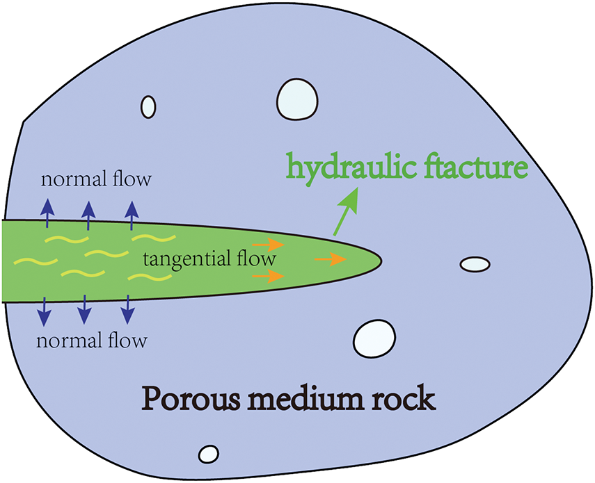
Figure 2: Fluid flow in propagating fracture
The normal flow equation is:
where qt and qb represent the normal flow rates into the top and bottom surfaces of the fracture, respectively. ct and cb are the corresponding fluid leak-off coefficients. pf is the fluid pressure within the fracture. pt and pb refer to the pore pressures at the top and bottom surfaces of the fracture, respectively.
Mass conservation within the fracture (for fluid volume) requires that the divergence of tangential flow plus the leak-off through the fracture surfaces equals the injection source. In weak form, the continuity (volume balance) for the fracture can be written including a Dirac delta for the injection point [21]:
where Q(t) is the injection rate, m2/s; δ(x,y) is the Dirac delta (which is zero except at the injection location).
2.3 Fracture Initiation and Propagation Criteria
(1) Initiation criteria
In the cohesive damage theory, fracture propagation initiates at the fracture tip or within the cohesive zone when cohesive forces are overcome, leading to gradual separation. Cohesive element adopts a traction-separation model, where linear elastic behavior is assumed prior to damage initiation. This linear elastic behavior represents the intrinsic elastic response of the material, defining the relationship between traction and separation before damage onset. Prior to damage initiation, stress and strain within the cohesive element follow a linear elastic relationship, expressed mathematically as follows:
where t represents the stress vector carried by the cohesive element, while tn, ts and tt denote the stresses in the normal and two tangential directions, respectively. K denotes the elastic stiffness matrix of the cohesive element.
The maximum nominal stress damage criterion specifies that damage in a cohesive element occurs when the stress in any direction exceeds the critical threshold. The criterion for initial damage is expressed as follows:
where
(2) Propagation criteria
Once the material within a cohesive element meets the initial damage criterion, the damage evolution criterion describes the progression of stiffness degradation. When the material satisfies the condition outlined in Eq. (12), the element enters the damage evolution stage, during which its stiffness gradually degrades under the influence of external forces. The governing equations for this stage are given by:
where
The variation of the damage variable D depends on the softening properties of the material and can be either linear or exponential, based on the effective displacement (as shown in Fig. 3). It is given by:
where
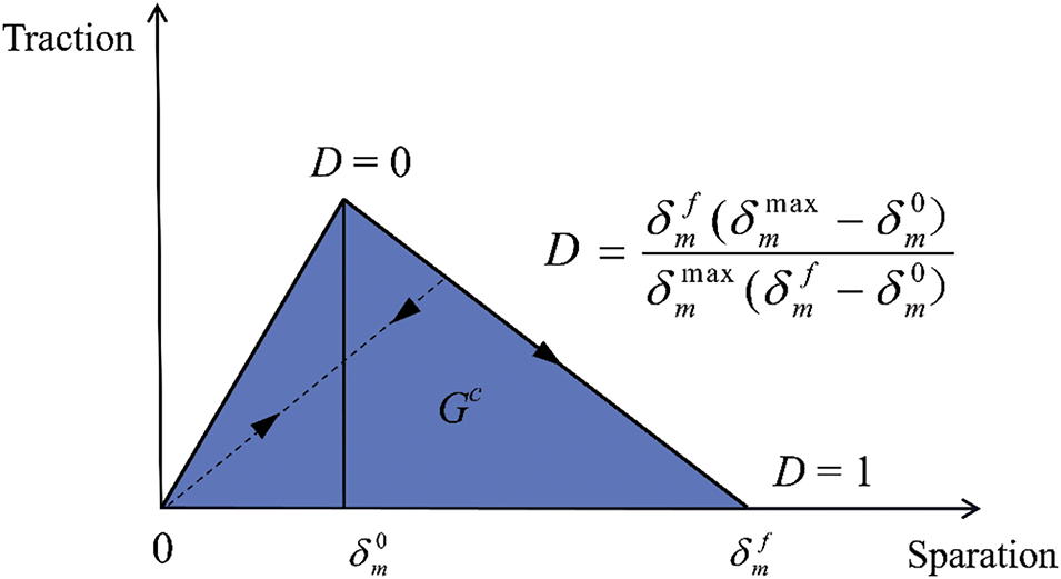
Figure 3: Cohesive traction-separation law
3 Model Validation and Numerical Example Setting
3.1 Embedding Process of the Cohesive Element
The fracture tip region is influenced by the mechanical behavior of the rock and pore pressure. To simulate the growth of fracture height, a cohesive element incorporating pore pressure degrees of freedom is introduced. This element is defined as a 6-node quadrilateral, with displacement degrees of freedom at the four corner nodes (nodes 1, 2, 3, and 4) and pore pressure degrees of freedom at the two middle nodes (nodes 5 and 6), as shown in Fig. 4.
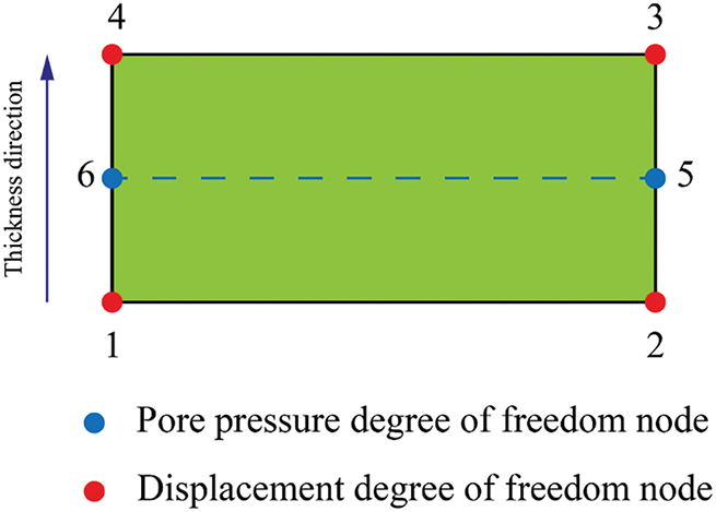
Figure 4: Cohesive elements with pore pressure nodes
The process of embedding the cohesive element into the finite element mesh involves three main steps: mesh processing, insertion of the cohesive element, and node merging, as shown in Fig. 5. The first step is to preprocess the global finite element mesh nodes (parent nodes) in the target area. Based on the mesh topology, the node numbers are updated to ensure the new sub-nodes remain independent. This step creates the interface needed to embed the cohesive element. Next, additional pore pressure nodes are inserted between the sub-nodes at the interface. Following the counterclockwise numbering principle, the independent sub-nodes are connected to the pore pressure nodes to form new interface elements. These interface elements are then aligned along the direction of the pore pressure nodes to form virtual double-node line elements, completing the embedding of the cohesive element. Finally, at the intersections of the cohesive elements in different directions, the pore pressure nodes are merged using a shared node method, ensuring fluid continuity throughout the region.
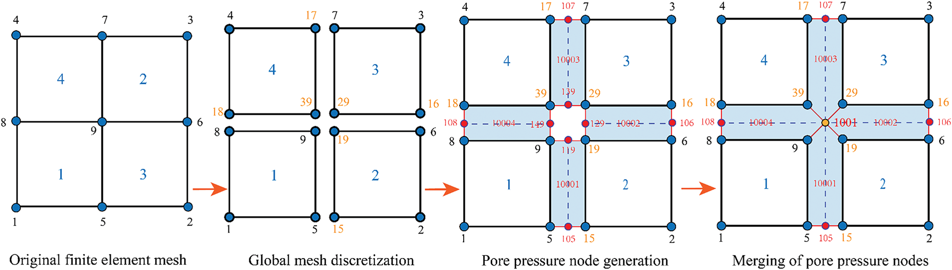
Figure 5: The process of embedding the zero-thickness cohesive element
3.2 Validation of the Numerical Model
In the absence of fluid leak-off, hydraulic fracture propagation involves two primary energy dissipation regimes: viscous-dominated and toughness-dominated. In the viscous-dominated regime, energy dissipation primarily results from the fracturing fluid flow. In the toughness-dominated regime, energy dissipation mainly arises from rock fracture and the creation of new fracture surfaces. Under plane strain conditions, these regimes can be distinguished using a dimensionless toughness parameter κ [22,23]:
where KIC is the Mode I fracture toughness,
where w is fracture width; x represents the distance from the injection point; l is the fracture length; and t is the injection time; The normalized coordinate along the fracture width is given by ξ = x/l. Specific parameters used for model validation are provided in Table 1.
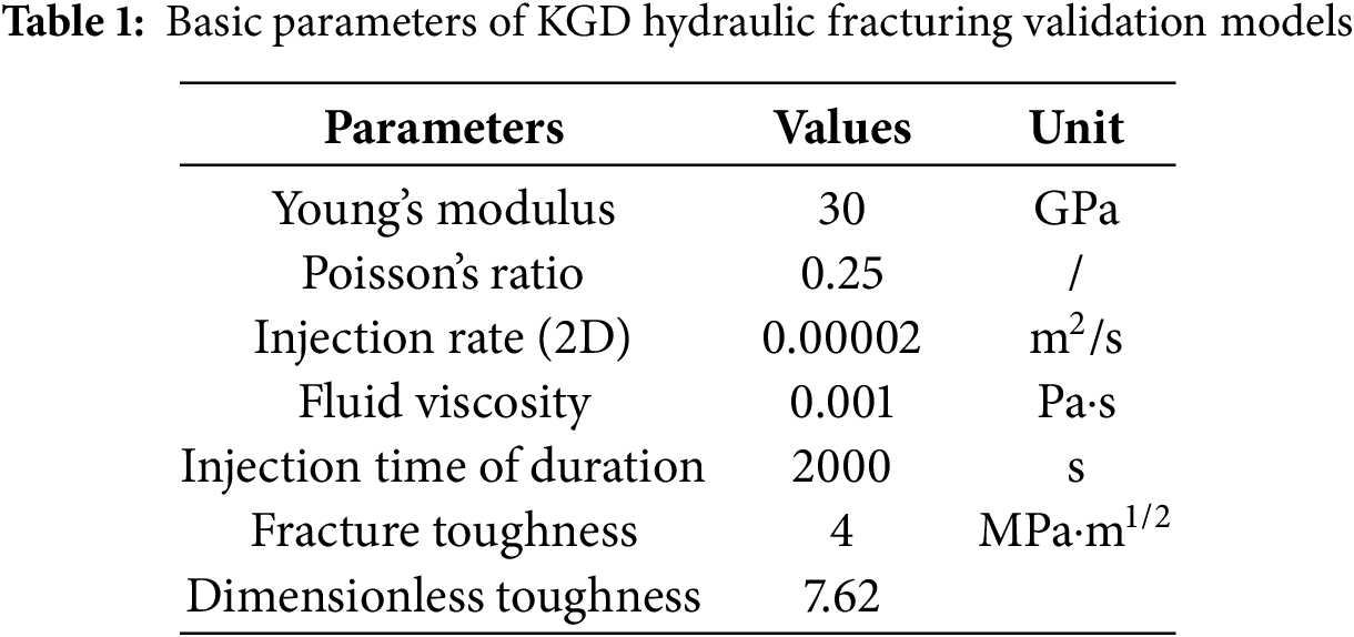
Using these inputs, our simulation produced fracture lengths and widths over time. Fig. 6 compares the numerical results (fracture length and width as functions of time) with the analytical KGD solution for a toughness-dominated fracture. Two main factors contribute to the minor discrepancies between the numerical and analytical solutions: (1) The analytical solution assumes an infinite domain, whereas the numerical solution is computed within a finite range. (2) The KGD model assumes the medium is impermeable; however, absolute impermeability cannot be fully realized in the numerical simulations using cohesive elements.
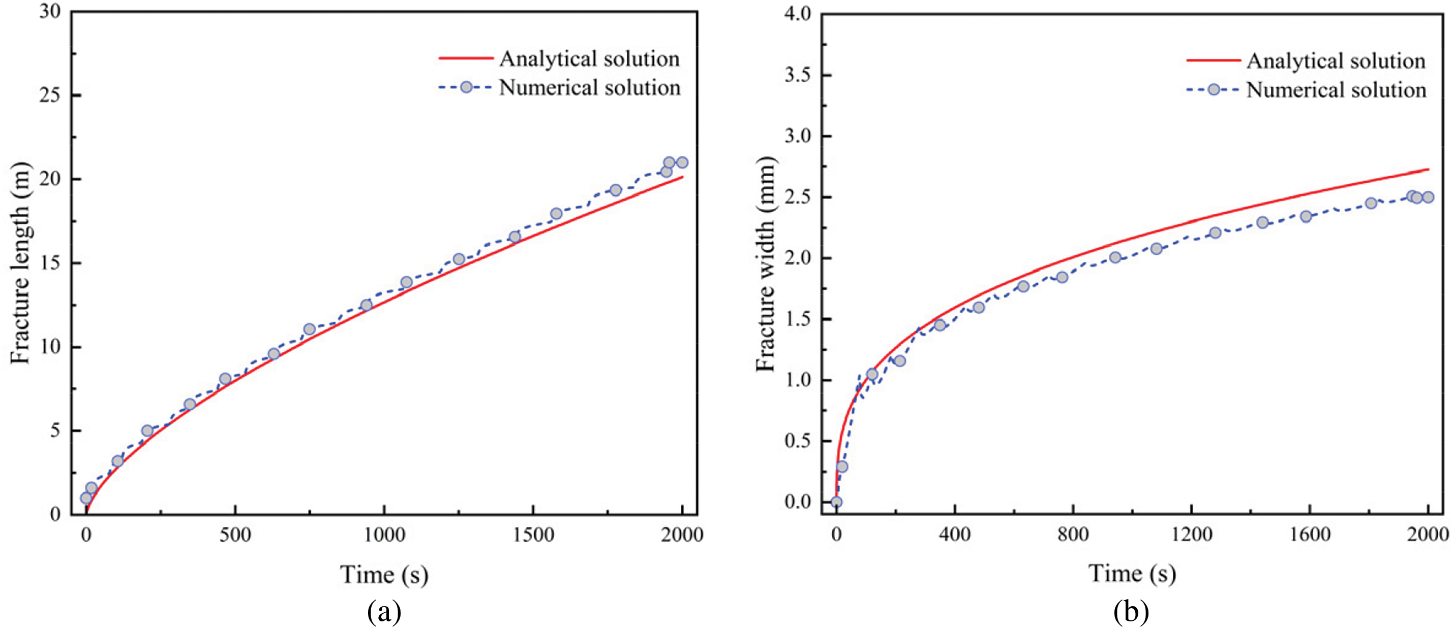
Figure 6: Comparison of numerical and analytical KGD solutions: (a) hydraulic fracture length and (b) hydraulic fracture width at fracture inlet
Before establishing the numerical model, it is essential to validate the mesh size to ensure a suitable balance between computational accuracy and efficiency. In this study, three different mesh sizes were tested: 0.25, 0.5, and 1 m. As shown in Fig. 7, the injection pressure curve fluctuated significantly with a grid size of 1 m, indicating lower computational accuracy. Conversely, decreasing the grid size to 0.25 m improved calculation accuracy but substantially increased computational time. Thus, after carefully balancing precision and efficiency, a grid size of 0.5 m was selected for subsequent simulations.
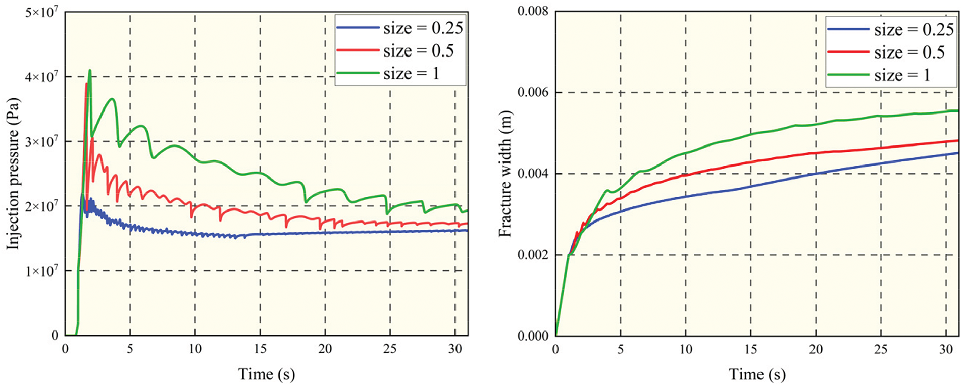
Figure 7: Mesh independence validation of injection pressure and fracture width
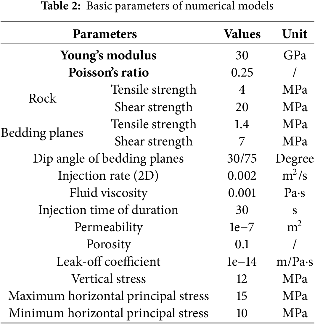
Reservoir fracturing operations commonly encounter bedding planes with low dip angles (0°–30°), which has prompted extensive research. However, more complex geological structures featuring high bedding dip angles (60°–85°) frequently occur in regions such as Xinjiang’s Tarim and Junggar Basins [25,26]. Given this context, this study specifically examines fracture height growth at formation dip angles of 30° and 75°, as illustrated in Fig. 8. The numerical model employed is a 2D plane strain configuration measuring 50 m × 50 m, divided into three distinct regions: upper and lower barrier layers, with the central section representing the reservoir. The injection point is positioned at the model’s center, maintaining an equal vertical distance of 10 m from both the upper and lower bedding planes. This setup ensures the hydraulic fracture encounters the bedding planes at consistent vertical distances for both dip angles. In the model, the minimum horizontal principal stress is oriented along the X-axis, while the vertical stress is aligned along the Y-axis. Initially, a geostatic equilibrium period of 1 s is implemented to stabilize the geo-stress and pore pressure before fracturing simulations commence. Fracturing fluid injection continues for 30 s, with an initial fracture width set at 0.002 m. The key parameters employed in the numerical model are summarized in Table 2. To maintain the comparability of simulation results, injection conditions remain consistent across all scenarios. During the parametric analysis examining fracture toughness contrast (Kc), stress differences between layers (Lc), and stress differences between the vertical stress and the horizontal minimum principal stress (SD), only the parameter under investigation is varied; all other parameters are held constant.
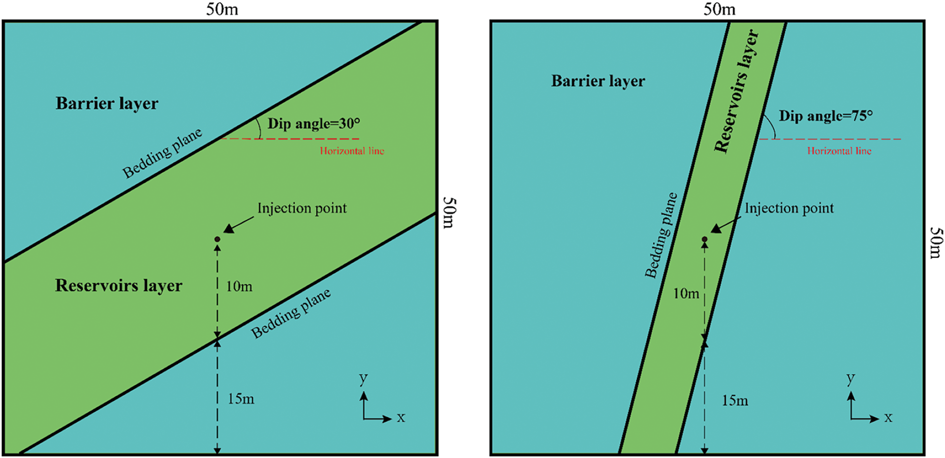
Figure 8: Numerical model setup and geometry
To quantify the impact of rock mechanics parameters on fracture height growth, these parameters were expressed in dimensionless forms. The parameters include the bedding shear strength (Bs), the bedding tensile strength (Bt), the toughness contrast between layers (Kc), the stress difference between layers (Lc), and the stress difference (SD). The bedding shear strength coefficient (Bs) is defined as the ratio of shear strength between the bedding plane and the rock matrix. Similarly, the bedding tensile strength coefficient (Bt) represents the tensile strength ratio between the bedding plane and the rock matrix. The toughness contrast between layers (Kc) is defined as the ratio of fracture toughness between the reservoir and barrier layers.
The stress difference between layers Lc is defined as:
where
Vertical to minimum horizontal stress difference SD is defined as:
where
Under different stress conditions and bedding dip angles, the fracture mode on bedding planes may vary. Under the influence of vertical stress, at lower dip angles, such as 30°, the shear stress acting on the bedding planes increases, leading to shear failure. In contrast, at higher dip angles, such as 75°, the formation tends to align with the vertical stress direction, increasing the tensile stress on the bedding planes and causing tensile failure. Therefore, this study specifically investigates how shear strength and tensile strength affect the vertical propagation of hydraulic fractures under these conditions. The key parameters used for numerical simulations are listed in Tables 3 and 4. Additional relevant parameters are provided in Table 2. In this study, interactions between hydraulic fractures and bedding planes are classified as either traversal or diversion. Traversal refers to situations where hydraulic fractures penetrate through bedding planes, whereas diversion describes cases where hydraulic fractures propagate along bedding planes. These behaviors are illustrated in Fig. 9.
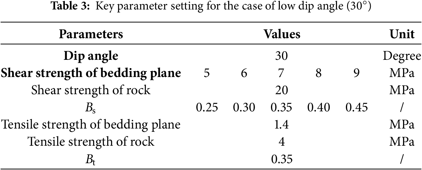
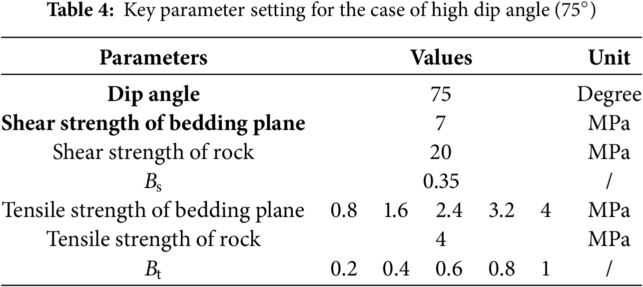
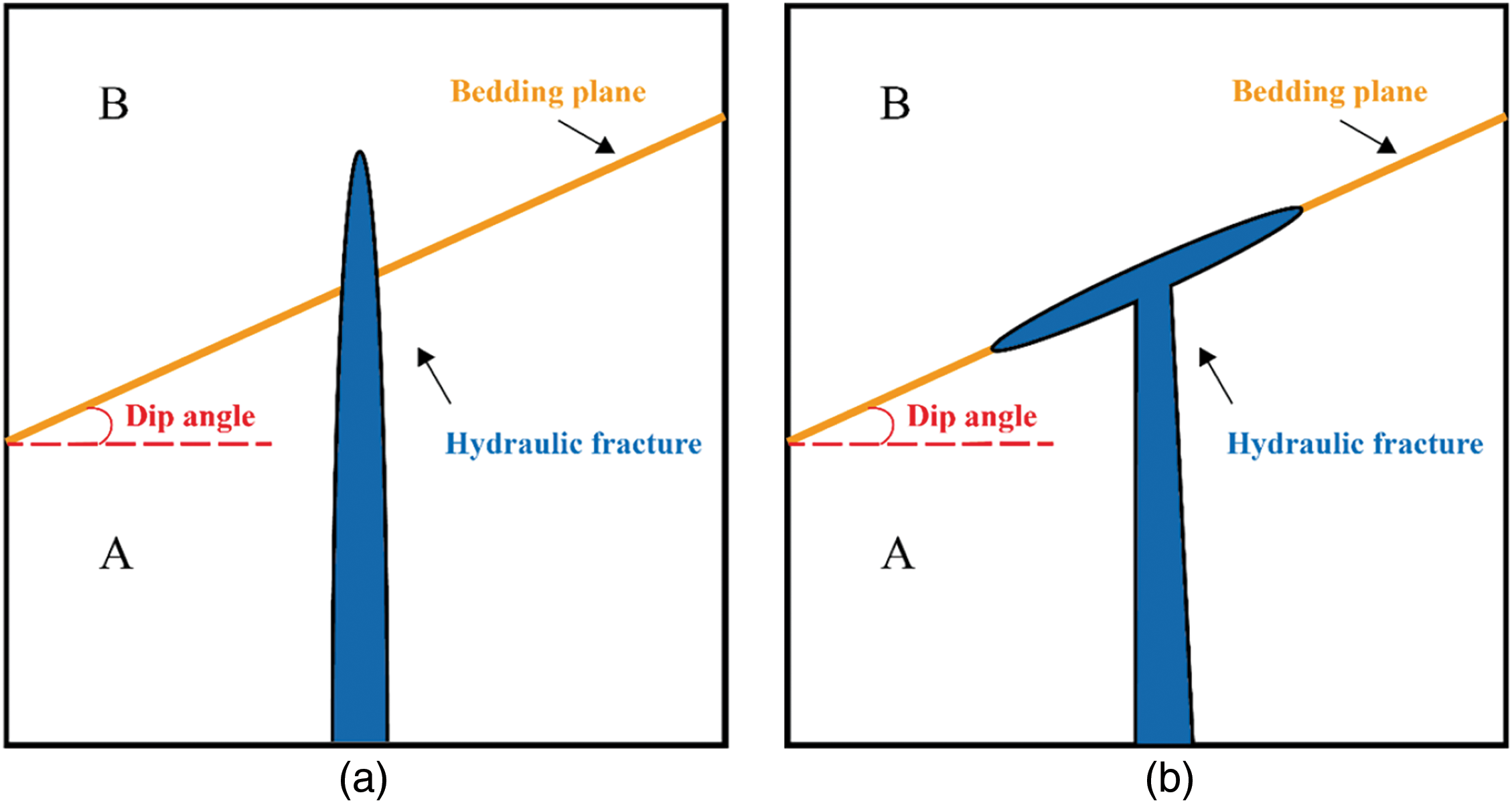
Figure 9: Fracture traversal and diversion behavior: (a) traversal; (b) diversion
4.1 Influence of Stress Difference between Layers on Height Growth
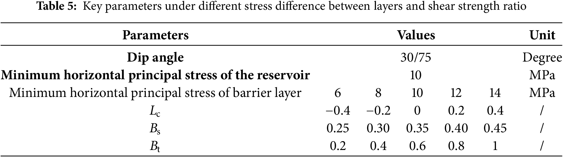
To examine the impact of stress difference between layers (Lc) on hydraulic fracture height growth, we tested Lc values of −0.4, −0.2, 0, 0.2, and 0.4. Correspondingly, the minimum horizontal principal stress of the barrier layer was set to 6, 8, 10, 12, and 14 MPa (Table 5). All other parameters are shown in Table 2.
(1) Low dip angle
At a low dip angle of 30°, the hydraulic fracture height growth is analyzed with respect to varying stress difference between layers (Lc) and shear strength ratio (Bs), as shown in Fig. 10. Higher Bs or lower Lc promote hydraulic fracture traversal through bedding planes. Elevated fluid pressure under these conditions drives vertical propagation into the barrier layer. Conversely, lower Bs or greater Lc enhance the tendency of hydraulic fractures to divert along bedding planes. The critical shear strength threshold between traversing and diversion behavior varies according to stress difference between layers. When Lc < 0.4, fracture propagation behavior becomes relatively insensitive to changes in stress difference between layers, making Bs the dominant factor influencing fracture height growth. However, when Lc = 0.4, hydraulic fractures predominantly divert along the bedding planes, primarily due to the strong barrier effect imposed by the stress field.
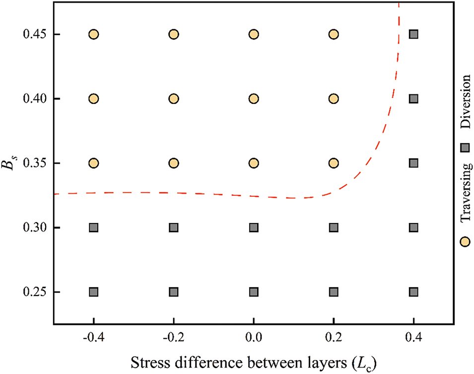
Figure 10: Numerical simulation results under the combined effect of bedding shear strength and stress difference between layers
Figs. 11 and 12 illustrate fracture morphology and stress distribution along the X-axis under different bedding shear strengths when Lc is 0.4. In these figures, PFOPEN represents the fracture width, while S and S11 represent the stress magnitude along the X-axis. The results show that as the bedding shear strength increases, the diversion distance of hydraulic fractures decreases, fracture width increases, and stress along the X-axis correspondingly rises.
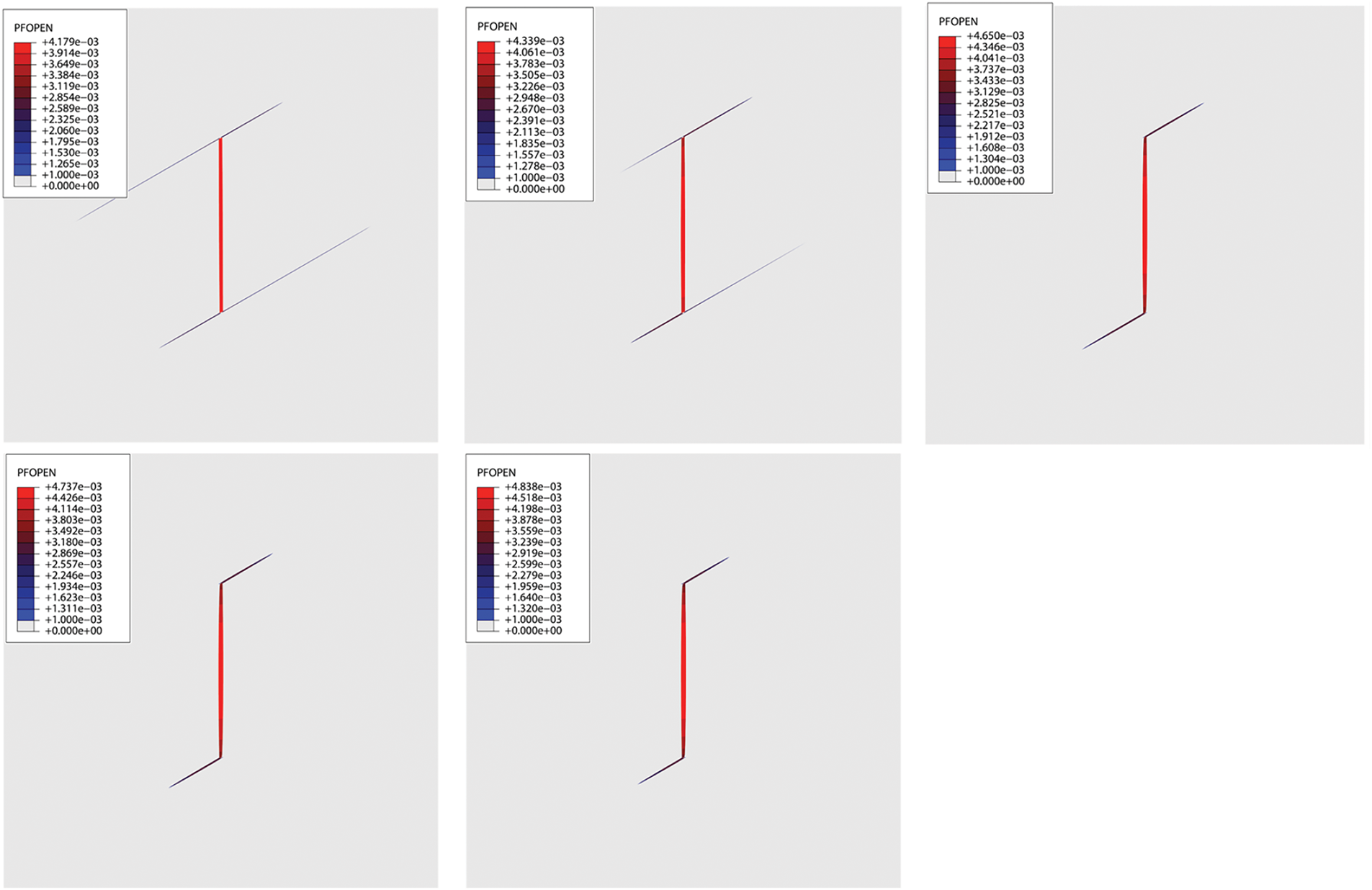
Figure 11: Fracture morphology at different bedding strength (Lc = 0.40)
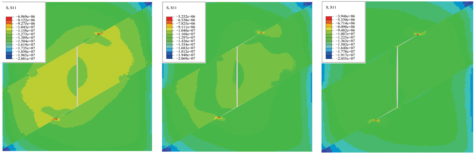
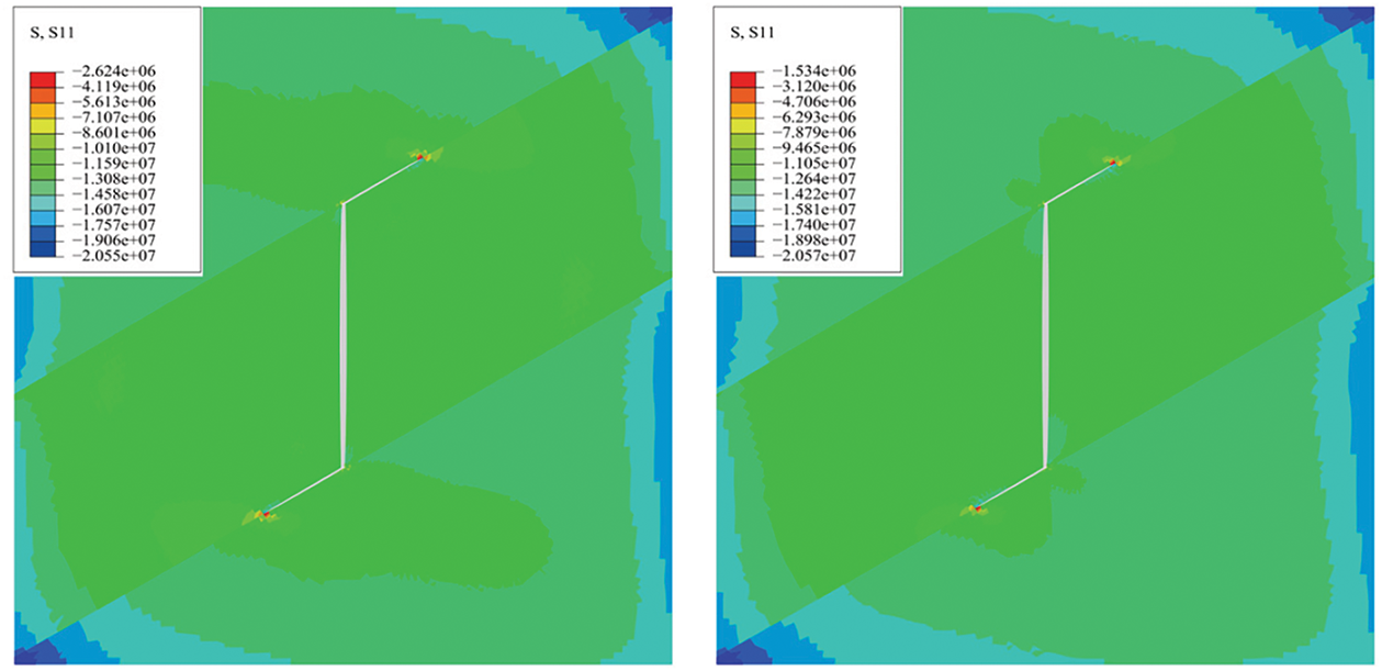
Figure 12: Stress distribution in the horizontal direction at different bedding strengths (Lc = 0.40)
(2) High dip angle
Fig. 13 illustrates fracture height growth at a high dip angle of 75°, considering varying Lc and Bt. The findings suggest that lower bedding plane tensile strength or larger stress difference between layers promote the diversion of hydraulic fractures along bedding planes. Furthermore, the threshold of tensile strength separating traversing and diversion behavior varies with the stress difference between layers. Unlike the scenario at low dip angles, the stress contrast between layers consistently impacts fracture propagation, regardless of whether the barrier layer exhibits higher or lower stress compared to the reservoir. When Lc < 0, hydraulic fractures traverse the bedding plane and propagate into the barrier layer under all examined tensile strength conditions. However, for Lc ≥ 0, the bedding tensile strength required to prevent fracture diversion increases nearly linearly with the minimum horizontal principal stress of the barrier layer.
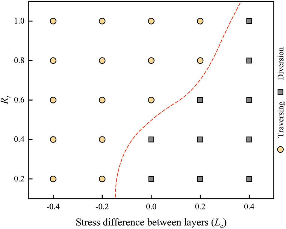
Figure 13: Numerical simulation results under the combined effect of tensile strength and stress difference between layers
For all bedding tensile strength scenarios examined, hydraulic fractures divert along bedding planes when Lc = 0.4, similar to the low dip angle case. This behavior indicates that stress difference between layers completely dominates fracture traversal or diversion behavior when Lc ≥ 0.4. Under such conditions, all hydraulic fractures divert along the bedding plane regardless of bedding strength, highlighting the significant control exerted by the high interlayer stress difference.
(3) Injection pressure and fracture width
Fig. 14 shows the injection pressure curves and fracture widths under different stress difference between layers at a tensile strength ratio of 1. The results indicate that the initiation and propagation pressures of hydraulic fractures increase with the interlayer stress difference. A larger Lc enhances the stress concentration in the adjacent barrier layers, resulting in greater compression of the reservoir layer. Consequently, this increased compression makes fracture initiation and vertical propagation more difficult. As a result, the fracture width increases, as illustrated in Fig. 14b.
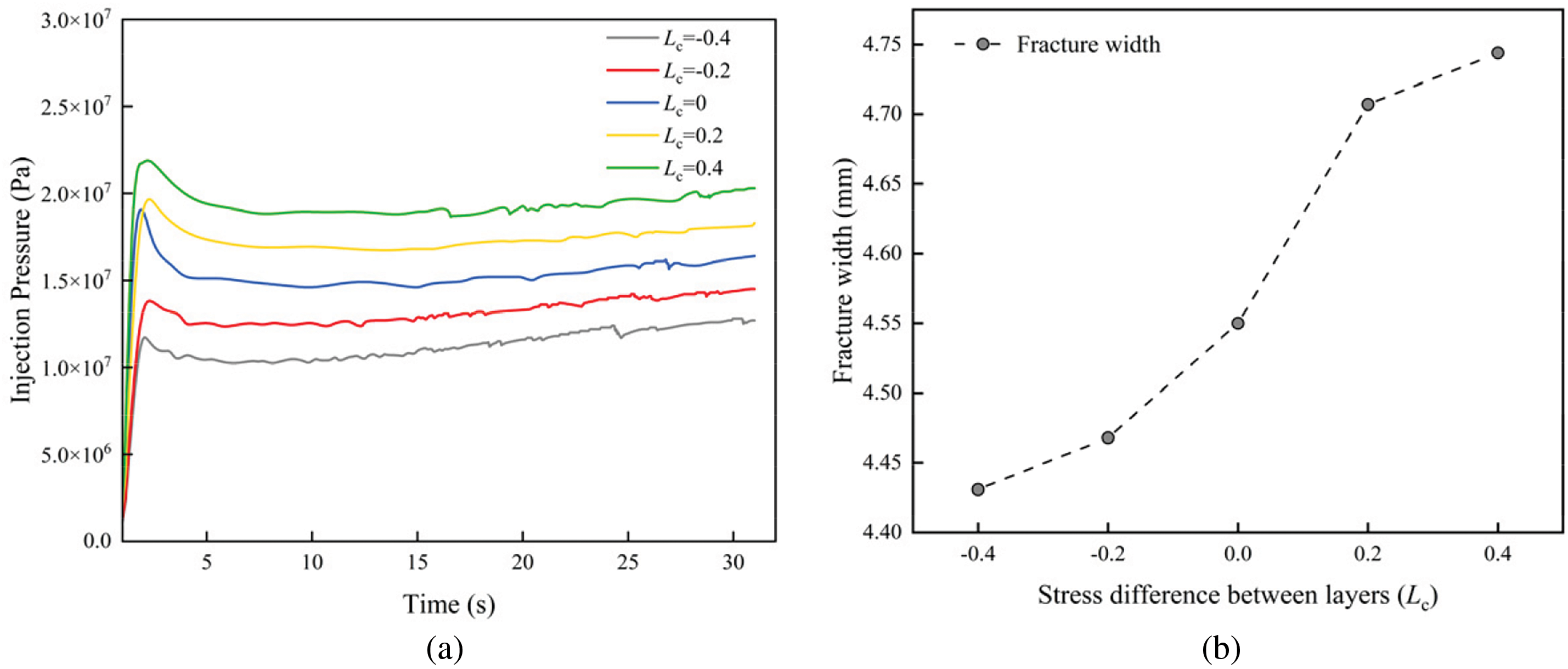
Figure 14: Injection pressure curves and fracture width at 75° dip angle (Bt = 1): (a) Injection pressure curves; (b) Fracture width
4.2 Influence of the Stress Difference on Height Growth
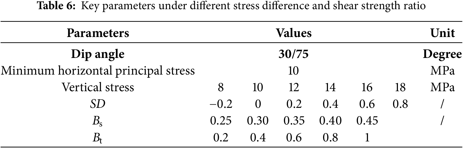
In stratified shale reservoirs, hydraulic fractures often exhibit non-planar growth patterns due to the combined effects of stress differences and bedding planes. In this study, vertical stress was varied to investigate how bedding planes influence fracture height growth under different stress conditions. The stress differences between the vertical stress and the horizontal minimum principal stress (SD) were set at −0.2, 0, 0.2, 0.4, 0.6, and 0.8, corresponding to vertical stress values of 8, 10, 12, 14, 16, and 18 MPa, respectively. The specific parameters are listed in Table 6, while all other parameters remain the same as those listed in Table 2.
(1) Low dip angle
At a low dip angle of 30°, fracture height growth was analyzed under varying SD and Bs, as shown in Fig. 15. Results indicate that lower Bs or smaller SD promote fracture propagation along the bedding planes, while higher Bs or larger SD favor hydraulic fracture traversal through the bedding planes. When SD < 0.2, vertical stress shows limited influence on further height growth; even with high bedding shear strength, hydraulic fractures tend to divert along the bedding plane. However, when SD ≥ 0.2, the shear strength threshold between fracture traversal and diversion becomes independent of the stress difference, making bedding shear strength the primary controlling factor. Under such conditions, shear failure predominantly occurs along bedding planes. When a hydraulic fracture encounters a bedding plane, it propagates along the path of lower fracture energy, which is determined by shear strengths of the bedding plane and the surrounding rock matrix. For example, at low bedding shear strengths (Bs < 0.35), hydraulic fractures are consistently contained by the bedding plane.
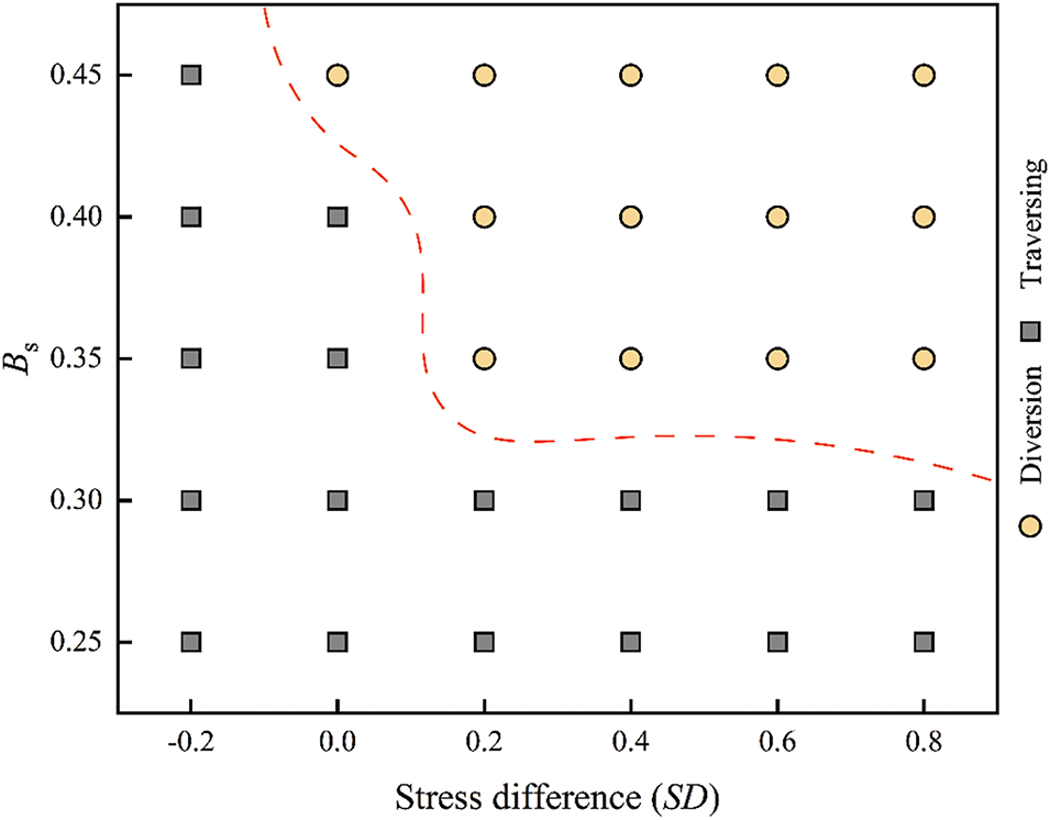
Figure 15: Numerical simulation results under the combined effect of bedding shear strength and stress difference
(2) High dip angle
Fig. 16 illustrates the growth of fracture height under different SD and Bt at a high dip angle of 75°. Results show that lower Bt or smaller SD promote hydraulic fracture diversion along bedding planes. Compared to the low dip angle scenario, hydraulic fractures at high dip angles show greater sensitivity to SD. Such sensitivity is attributed to the fact that higher stress differences promote shear failure along bedding planes. Based on the analysis in Section 4.2 (1), hydraulic fractures penetrate the bedding plane when Bs ≥ 0.35. In this study, the bedding plane is assigned a higher shear strength (Bs = 0.35) under high dip angle. Therefore, at high stress differences (SD > 0.2), the differences in fracture behavior between low and high dip angles primarily stem from differences in Bs. When SD ≤ 0.2, fractures divert only when the bedding tensile strength is low. This suggests that at low stress differences and high dip angles, the tensile strength of the bedding plane significantly influences fracture height growth.
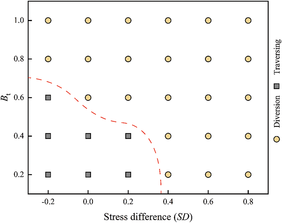
Figure 16: Numerical simulation results under the combined effect of bedding shear strength and horizontal stress difference
Fig. 17 shows fracture morphologies under different stress differences between the vertical stress and the horizontal minimum principal stress (SD). At a low stress difference (SD = −0.4), hydraulic fractures propagate horizontally instead of vertically (Fig. 17a). This behavior is typical when the vertical stress is lower than the minimum horizontal principal stress—a condition often observed in shallow coal and rock layers (less than 400 m depth). With low bedding strength and small stress difference (SD = 0), fractures still propagate easily along bedding planes due to reduced resistance (Fig. 17b). However, under conditions of high bedding strength and elevated horizontal stress difference (SD = 0.4), increased normal stress on the bedding plane enhances resistance, causing fractures to more frequently traverse the bedding plane (Fig. 17c).
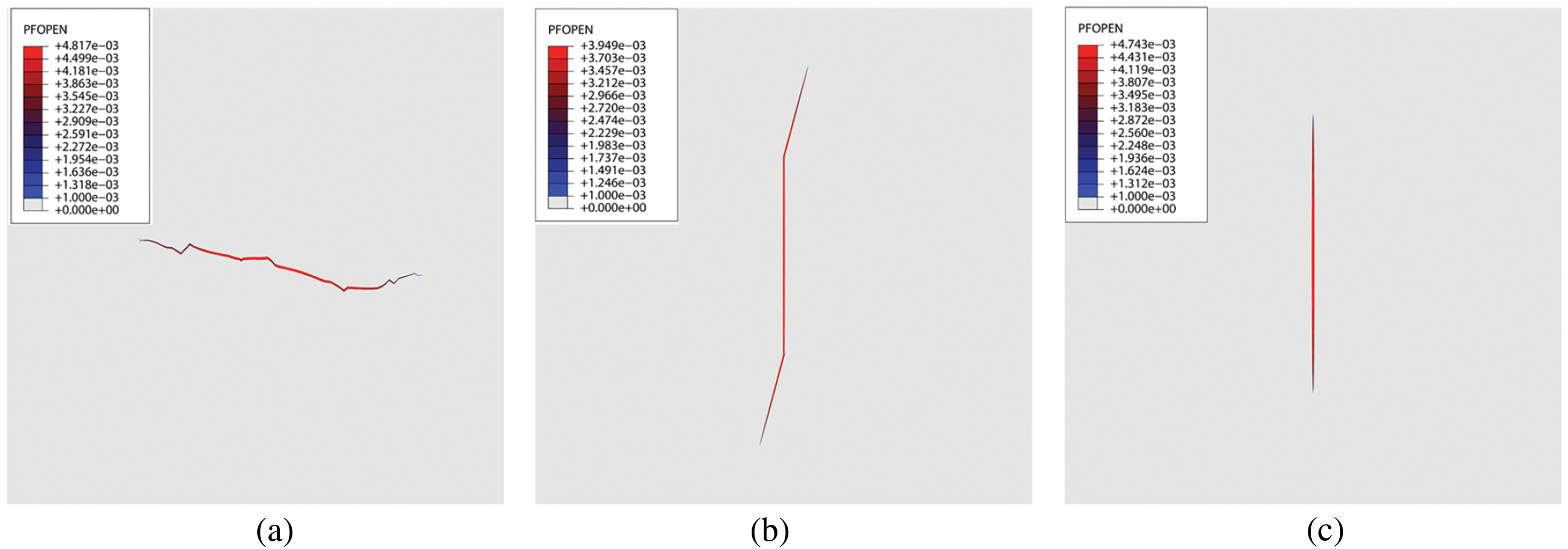
Figure 17: Fracture morphology at different horizontal stress difference: (a) SD = −0.4; (b) SD = 0; (c) SD = 0.4 (3) Injection pressure and fracture width
Fig. 18 shows the injection pressure curves and fracture widths under different SD when Bs is 0.45. As the stress difference increases, both the initiation and propagation pressures of hydraulic fractures rise. At higher stress differences, more energy is required to induce rock fracturing, which increases the resistance to fracture propagation. As a result, a higher net pressure is needed to overcome the high horizontal stress difference. With constant injection conditions, an increased stress difference drives the fracture to grow vertically, resulting in a reduced width.
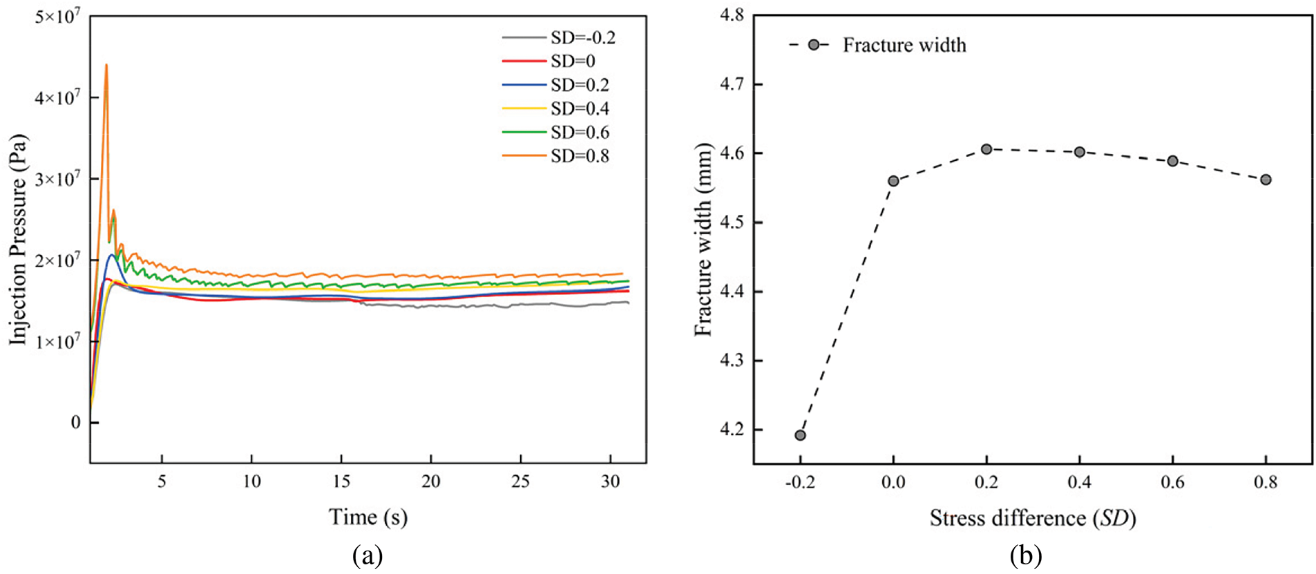
Figure 18: Injection pressure curves and fracture width at dip angle = 30° (Bs = 0.45): (a) Injection pressure curves; (b) Fracture width
4.3 Influence of Toughness Contrast on Height Growth
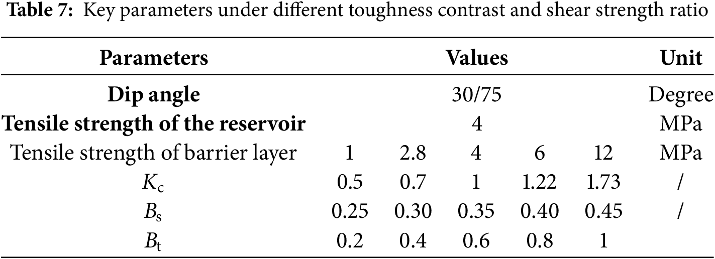
To study the effect of fracture toughness contrast between layers on hydraulic fracture height growth, the fracture toughness (Kc) was assigned values of 0.5, 0.83, 1, 1.22, and 1.73. These values correspond to barrier rock matrix tensile strengths of 1, 2.8, 4, 6, and 12 MPa, respectively, as shown in Table 7. Other parameters remain the same as those in Table 2. The fracture toughness of the rock is calculated using the following equation [27]:
where KIC is the fracture toughness, v is Poisson’s ratio, E is the elasticity modulus, T is the maximum critical stress, and
(1) Low dip angle
At a low dip angle of 30°, hydraulic fracture growth was examined under various Kc and Bs conditions, as shown in Fig. 19. The results indicate that a higher Bs or a lower Kc requires less energy for the fluid to overcome resistance, thereby facilitating hydraulic fracture propagation across the bedding plane. Conversely, a lower Bs or a higher Kc promote the hydraulic fracture diversion along the bedding plane.
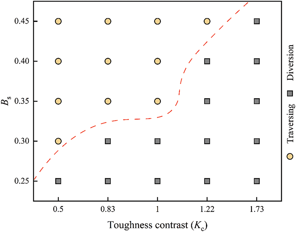
Figure 19: Numerical simulation results under the combined effect of bedding shear strength and toughness contrast
The threshold shear strength that differentiates between traversing and diversion behavior depends on the value of Kc. As Kc increases, the shear strength required to resist hydraulic fracture propagation along the bedding planes increases. When Kc is 0.5, the fracture toughness of the barrier rock (1.27 MPa
(2) High dip angle
At a high dip angle of 75°, fracture height growth under different Kc and Bt conditions is presented in Fig. 20. Similar to the low dip angle case, lower Bt or larger Kc promote the hydraulic fractures be constrained by the bedding planes. The tensile strength threshold that determines whether the fracture traverses or diverts varies with the fracture toughness contrast. When Kc is 0.5, hydraulic fractures penetrate the bedding planes and propagate into the barrier layers regardless of the bedding tensile strength. However, when Kc is 1.73, hydraulic fractures extend along the bedding plane for all tensile strength levels, indicating that fracture toughness contrast exerts a dominant effect on hydraulic fracture behavior relative to the bedding plane strength.
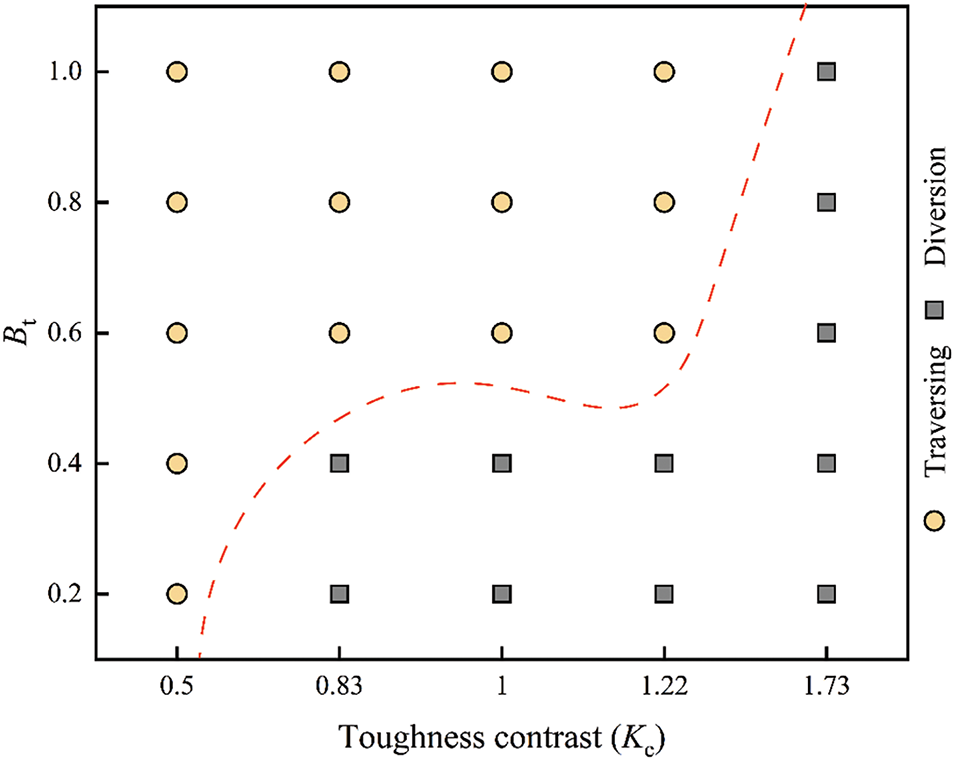
Figure 20: Numerical simulation results for the combined effect of bedding tensile strength and toughness contrast
Fig. 21 shows the horizontal displacements (U, U1) for both low (30°) and high (75°) dip angles when hydraulic fractures divert under a fracture toughness contrast of 1.73 and high bedding strength (Bs = 0.45 or Bt = 1). Here, U and U1 represent the displacement along the x-axis. The results indicate that horizontal displacement is greater at the high dip angle compared to the low dip angle. Moreover, the propagation distance of the hydraulic fracture along the bedding plane is longer at the low dip angle. This suggests that under a high toughness contrast, more fracturing fluid leaks through low dip bedding planes, while less fluid leaks through high dip bedding planes.
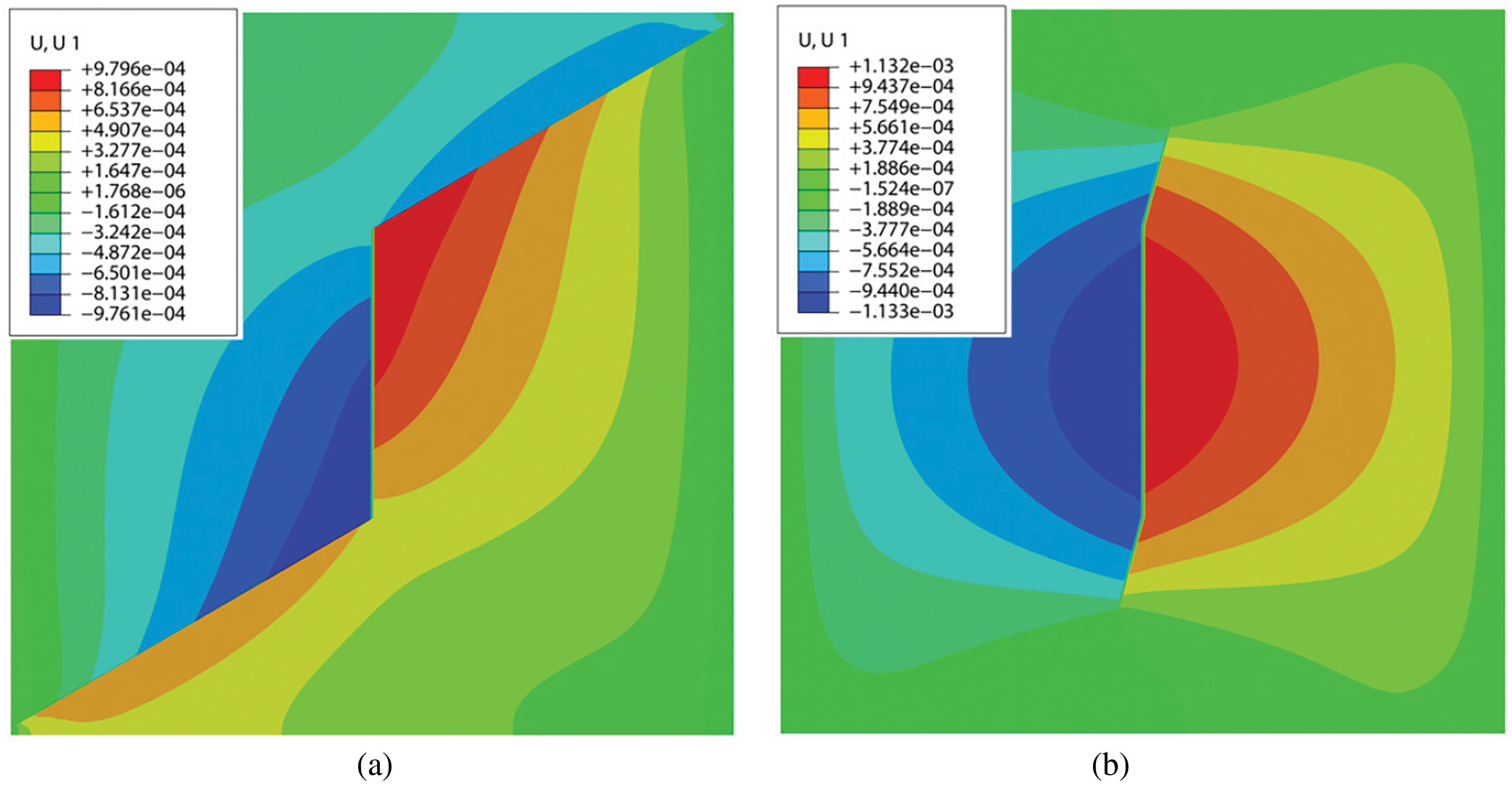
Figure 21: Horizontal displacements: (a) Low dip angle of 30°; (b) High dip angle of 75°
(3) Injection pressure and fracture width
Fig. 22 shows the injection pressure curves and fracture widths for different fracture toughness contrasts. When Kc < 1.73, hydraulic fractures penetrate the bedding planes. As Kc increases, the propagation pressure decreases while fracture width increases. For a high fracture toughness contrast (Kc = 1.73), the barrier layer exhibits significant resistance to fracture propagation. Due to the combined effect of high shear strength in the barrier layers and the high fracture toughness contrast, vertical fracture propagation is inhibited, resulting in fluid accumulation within the fracture. Once the fluid pressure exceeds the fracture pressure of the bedding plane, the fracture diverts along the bedding plane. This diversion further reduces the propagation pressure (Fig. 22a) and results in a narrower fracture width (Fig. 22b). At a fluid injection time of 30.49 s, the hydraulic fracture nearly reaches the model boundary, as indicated by the red dashed box in Fig. 23. In the following time step, the fracture breaches the boundary, leading to significant fluid loss, a drop in pressure, and further narrowing of the fracture.
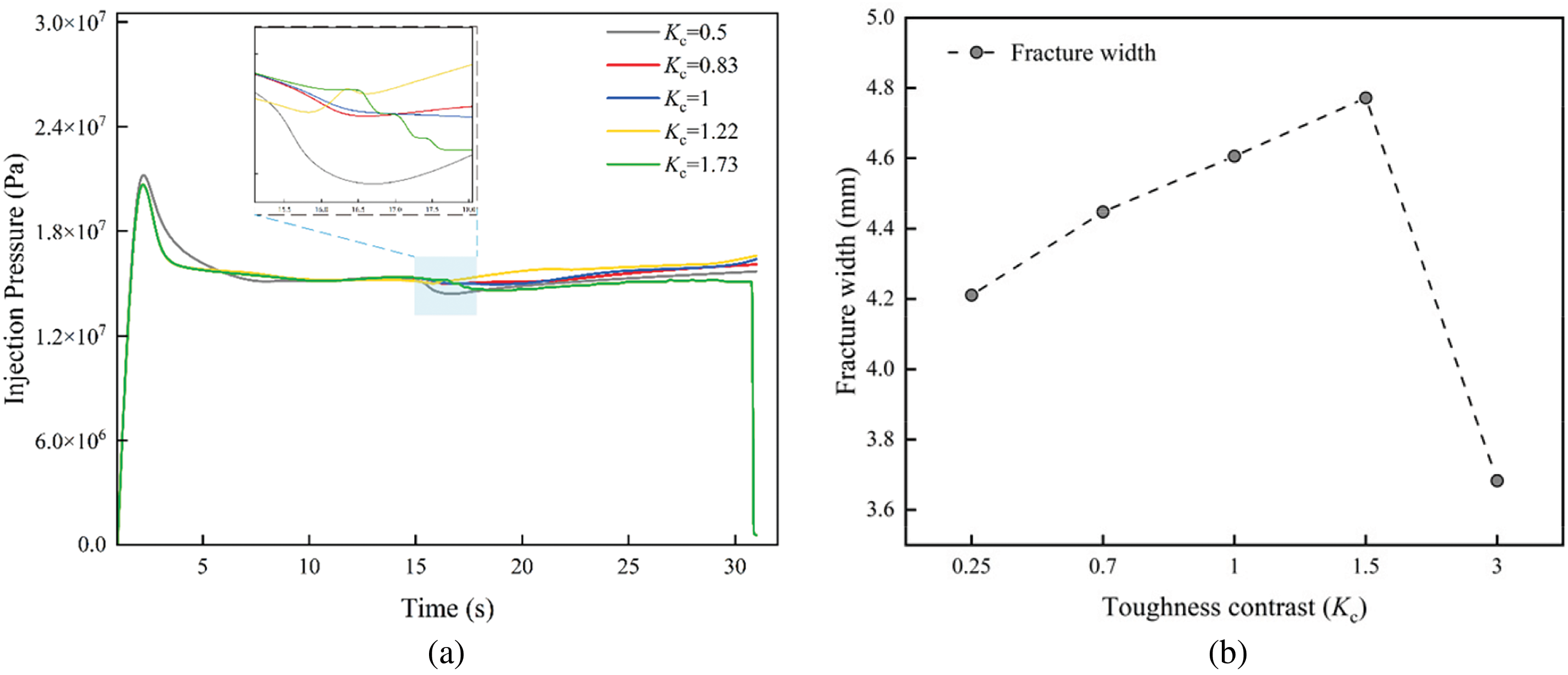
Figure 22: Injection pressure curves and fracture width at dip angle = 30° (Bs = 0.45): (a) Injection pressure curves; (b) Fracture width
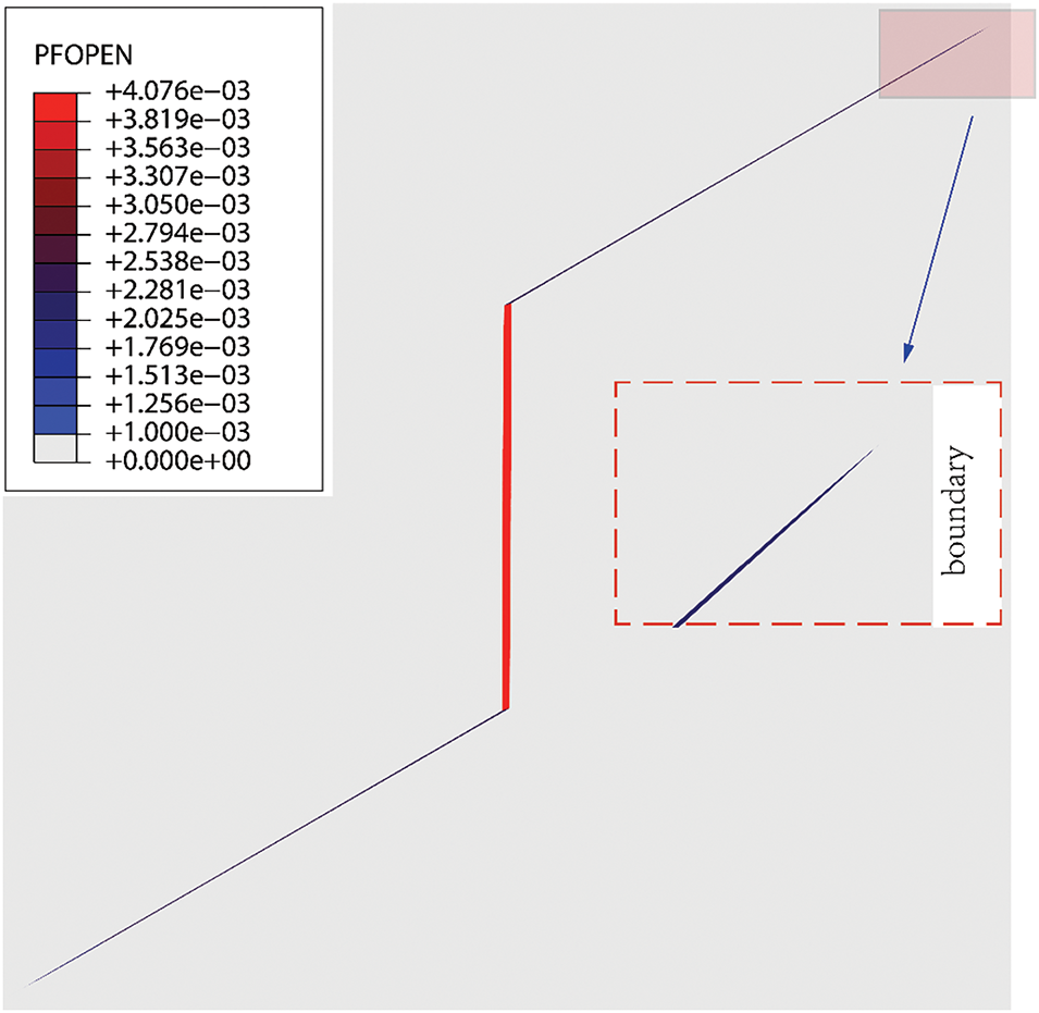
Figure 23: Fracture reaching model boundary under high toughness contrast at 30° dip angle (Kc = 1.73)
This study conducted numerical simulations using a finite element method with zero-thickness cohesive elements to investigate the height growth of hydraulic fractures under the combined effects of the bedding planes (including bedding strength and dip angle), the toughness contrast (Kc), the stress difference between layers (Lc), and the stress difference between the vertical stress and the horizontal minimum principal stress (SD). The analysis focused on the behavior of hydraulic fractures as they traverse or divert based on each parameter. The key findings are as follows:
(1) Lower bedding strength, reduced stress difference (SD), higher stress difference between layers (Lc), and greater toughness contrast (Kc) promote hydraulic fracture containment within the reservoir layer. These conditions drive fractures to propagate along bedding planes rather than vertically into the barrier layers. In contrast, elevated bedding strength, increased SD, diminished Lc, and lower Kc promote vertical fracture penetration through bedding planes. Such vertical growth can be suppressed in reservoirs with weak interfacial strength and high stress/toughness barriers. In field terms, this suggests that in reservoirs with weak interfaces and high stress or toughness barriers, fractures will remain more confined in height. Optimizing injection parameters (such as injection rate and fluid viscosity) can help limit excessive height growth when such unfavorable conditions exist, thereby improving reservoir stimulation efficiency while avoiding fracture growth into unwanted layers.
(2) For a given bedding strength, increasing either the Lc or SD increases the fracture initiation and propagation pressures required. Moreover, a higher Lc leads to a wider fracture (greater width) within the reservoir, as the fracture extends laterally along the interface instead of vertically. A higher Kc similarly promotes shear slip along the bedding plane and reduces the pressure needed once the fracture diverts. In our simulations, when Kc = 1.73, the high toughness contrast caused the fracture to slide along the bedding plane, accompanied by a noticeable reduction in propagation pressure.
(3) When the vertical stress is sufficiently small relative to horizontal (SD < −0.2), hydraulic fractures did not propagate upward at all—instead, they extended laterally, essentially forming horizontal fractures. Conversely, when Lc is 0.4, fractures consistently divert along bedding planes regardless of other parameters. Stronger bedding planes shorten lateral extension distances while amplifying horizontal stress fields.
Acknowledgement: Not applicable.
Funding Statement: This research was funded by the National Natural Science Foundation of China (No. 52204052), the National Natural Science Foundation of China (No. U23B20156), and the Sichuan Science and Technology Program (No. 2023NSFSC0933).
Author Contributions: The authors confirm contribution to the paper as follows: Conceptualization, Manqing Qian and Xiyu Chen; methodology, Xiyu Chen; software, Manqing Qian; validation, Manqing Qian and Yongming Li; formal analysis, Manqing Qian; investigation, Yongming Li; resources, Xiyu Chen; data curation, Manqing Qian; writing—original draft preparation, Manqing Qian; writing—review and editing, Xiyu Chen; visualization, Manqing Qian; supervision, Yongming Li; project administration, Yongming Li; funding acquisition, Yongming Li. All authors reviewed the results and approved the final version of the manuscript.
Availability of Data and Materials: The data that support the findings of this study are available on request from the corresponding author.
Ethics Approval: Not applicable.
Conflicts of Interest: The authors declare no conflicts of interest to report regarding the present study.
Nomenclature
| Bs | Bedding shear strength |
| Bt | Bedding tensile strength |
| Kc | Toughness contrast between layers |
| SD | Stress difference |
| Lc | Stress difference between layers |
| Q | Injection rate |
| E | Young’s modulus |
| v | Poisson’s ratio |
| Fluid viscosity | |
| KIC | The Mode I fracture toughness |
| κ | Dimensionless toughness |
| w | Fracture width at inlet |
| l | Fracture length |
References
1. Simonson ER, Abou-Sayed AS, Clifton RJ. Containment of massive hydraulic fractures. Soc Petrol Eng J. 1978;18(1):27–32. doi:10.2118/6089-PA. [Google Scholar] [PubMed] [CrossRef]
2. Palmer ID, Carroll HB Jr. Three-dimensional hydraulic fracture propagation in the presence of stress variations. Soc Petrol Eng J. 1983;23(6):870–8. doi:10.2118/10849-PA. [Google Scholar] [PubMed] [CrossRef]
3. Ali Daneshy A. Factors controlling the vertical growth of hydraulic fractures. In: SPE Hydraulic Fracturing Technology Conference; 2009 Jan 19–21; The Woodlands, TX, USA: SPE; 2009. SPE-118789-MS. doi:10.2118/118789-ms. [Google Scholar] [PubMed] [CrossRef]
4. Nie Y, Wang X, Wu B, Zhang G, Gamage RP, Li S, et al. Influences of the stress ratio and local micro mineral aggregates on small fatigue crack propagation in the shale containing bedding planes. Int J Rock Mech Min Sci. 2025;185(6):105980. doi:10.1016/j.ijrmms.2024.105980. [Google Scholar] [CrossRef]
5. Rutledge J, Weng X, Yu X, Chapman C, Leaney S. Bedding-plane slip as a microseismic source during hydraulic fracturing. In: SEG Technical Program Expanded Abstracts 2016; 2016; Dallas, TX, USA: Society of Exploration Geophysicists; 2016. p. 2555–9. doi:10.1190/segam2016-13966680.1. [Google Scholar] [CrossRef]
6. Daneshy AA. Hydraulic fracture propagation in layered formations. Soc Petrol Eng J. 1978;18(1):33–41. doi:10.2118/6088-PA. [Google Scholar] [PubMed] [CrossRef]
7. Xu W, Prioul R, Berard T, Weng X, Kresse O. Barriers to hydraulic fracture height growth: a new model for sliding interfaces. In: SPE Hydraulic Fracturing Technology Conference and Exhibition; 2019 Feb 5–7; The Woodlands, TX, USA: SPE; 2019. D011S002R005. doi:10.2118/194327-ms. [Google Scholar] [PubMed] [CrossRef]
8. Huang L, Li B, Wu B, Li C, Wang J, Cai H. Study on the extension mechanism of hydraulic fractures in bed-ding coal. Theor Appl Fract Mech. 2024;131(3):104431. doi:10.1016/j.tafmec.2024.104431. [Google Scholar] [CrossRef]
9. Gudmundsson A, Brenner SL. How hydrofractures become arrested. Terra N. 2001;13(6):456–62. doi:10.1046/j.1365-3121.2001.00380.x. [Google Scholar] [CrossRef]
10. Jeffrey RG, Bunger A. A detailed comparison of experimental and numerical data on hydraulic fracture height growth through stress contrasts. SPE J. 2009;14(3):413–22. doi:10.2118/106030-PA. [Google Scholar] [PubMed] [CrossRef]
11. Huang L, Dontsov E, Fu H, Lei Y, Weng D, Zhang F. Hydraulic fracture height growth in layered rocks: per-spective from DEM simulation of different propagation regimes. Int J Solids Struct. 2022;238(12):111395. doi:10.1016/j.ijsolstr.2021.111395. [Google Scholar] [CrossRef]
12. Xie J, Tang J, Yong R, Fan Y, Zuo L, Chen X, et al. A 3-D hydraulic fracture propagation model applied for shale gas reservoirs with multiple bedding planes. Eng Fract Mech. 2020;228(2):106872. doi:10.1016/j.engfracmech.2020.106872. [Google Scholar] [CrossRef]
13. Zheng Y, He R, Huang L, Bai Y, Wang C, Chen W, et al. Exploring the effect of engineering parameters on the penetration of hydraulic fractures through bedding planes in different propagation regimes. Comput Geotech. 2022;146(7):104736. doi:10.1016/j.compgeo.2022.104736. [Google Scholar] [CrossRef]
14. Cong Z, Li Y, Tang J, Martyushev DA, Hubuqin, Yang F. Numerical simulation of hydraulic fracture height layer-through propagation based on three-dimensional lattice method. Eng Fract Mech. 2022;264:108331. doi:10.1016/j.engfracmech.2022.108331. [Google Scholar] [CrossRef]
15. Ma J, Li X, Yao Q, Tan K. Numerical simulation of hydraulic fracture extension patterns at the interface of coal-measure composite rock mass with Cohesive Zone Model. J Clean Prod. 2023;426:139001. doi:10.1016/j.jclepro.2023.139001. [Google Scholar] [CrossRef]
16. Wang Y, Hou B, Wang D, Jia Z. Features of fracture height propagation in cross-layer fracturing of shale oil reservoirs. Petrol Explor Dev. 2021;48(2):469–79. doi:10.1016/S1876-3804(21)60038-1. [Google Scholar] [CrossRef]
17. Biot MA. General theory of three-dimensional consolidation. J Appl Phys. 1941;12(2):155–64. doi:10.1063/1.1712886. [Google Scholar] [CrossRef]
18. Zienkiewicz OC, Taylor RL. The finite element method. 5th ed. London, UK: Elsevier Pte Ltd.; 2005. [Google Scholar]
19. Wang B, Zhou FJ, Wang D, Liang T, Yuan L, Hu J. Numerical simulation on near-wellbore temporary plugging and diverting during refracturing using XFEM-Based CZM. J Nat Gas Sci Eng. 2018;55(2):368–81. doi:10.1016/j.jngse.2018.05.009. [Google Scholar] [CrossRef]
20. Boone TJ, Ingraffea A. A numerical procedure for simulation of hydraulically-driven fracture propagation in poroelastic media. Int J Numer Anal Meth Geomech. 1990;14(1):27–47. doi:10.1002/nag.1610140103. [Google Scholar] [CrossRef]
21. Peirce A, Detournay E. An implicit level set method for modeling hydraulically driven fractures. Comput Meth Appl Mech Eng. 2008;197(33–40):2858–85. doi:10.1016/j.cma.2008.01.013. [Google Scholar] [CrossRef]
22. Detournay E. Propagation regimes of fluid-driven fractures in impermeable rocks. Int J Geomech. 2004;4(1):35–45. doi:10.1061/(ASCE)1532-3641(2004)4:1(35). [Google Scholar] [CrossRef]
23. Cheng S, Wu B, Zhang X, Huppert HE, Jeffrey RG. How energy dissipation mode controls the evolution of multiple plane-strain hydraulic fractures under isotropic stresses. JGR Solid Earth. 2024;129(8):e2024JB029179. doi:10.1029/2024JB029179. [Google Scholar] [CrossRef]
24. Dontsov EV. An approximate solution for a plane strain hydraulic fracture that accounts for fracture toughness, fluid viscosity, and leak-off. Int J Fract. 2017;205(2):221–37. doi:10.1007/s10704-017-0192-4. [Google Scholar] [CrossRef]
25. Tang S, Liu S, Tang D, Tao S, Zhang A, Pu Y, et al. Occurrence of fluids in high dip angled coal measures: geological and geochemical assessments for southern Junggar Basin. China J Nat Gas Sci Eng. 2021;88(4):103827. doi:10.1016/j.jngse.2021.103827. [Google Scholar] [CrossRef]
26. Kang J, Fu X, Gao L, Liang S. Production profile characteristics of large dip angle coal reservoir and its impact on coalbed methane production: a case study on the Fukang west block, southern Junggar Basin. China J Petrol Sci Eng. 2018;171:99–114. doi:10.1016/j.petrol.2018.07.044. [Google Scholar] [CrossRef]
27. Haddad M, Sepehrnoori K. XFEM-based CZM for the simulation of 3D multiple-cluster hydraulic fracturing in quasi-brittle shale formations. Rock Mech Rock Eng. 2016;49(12):4731–48. doi:10.1007/s00603-016-1057-2. [Google Scholar] [CrossRef]
Cite This Article
 Copyright © 2025 The Author(s). Published by Tech Science Press.
This work is licensed under a Creative Commons Attribution 4.0 International License , which permits unrestricted use, distribution, and reproduction in any medium, provided the original work is properly cited.
 Downloads
 Citation Tools