
 Submit a Paper
 Propose a Special lssue
 Open Access
ARTICLE

Evaluation of Estimated Ultimate Recovery for Shale Gas Infill Wells Considering Inter-Well Crossflow Dynamics
1 Geological Exploration and Development Research Institute, CNPC Chuanqing Drilling Engineering Company Limited, Chengdu, 610000, China
2 Sichuan Yuesheng Oil & Gas Field Technical Service Company Limited, Chengdu, 610000, China
3 Sichuan Hengyi Petroleum Technology Service Company Limited, Chengdu, 610000, China
4 Sichuan Changning Natural Gas Development Company Limited, Chengdu, 610000, China
5 CNPC Chuanqing Drilling Engineering Company Limited Sulige Project Management Department, Erdos, 017300, China
* Corresponding Authors: Cuiping Yuan. Email: ; Sicun Zhong. Email:
(This article belongs to the Special Issue: Fluid and Thermal Dynamics in the Development of Unconventional Resources III)
Fluid Dynamics & Materials Processing 2025, 21(7), 1689-1710. https://doi.org/10.32604/fdmp.2025.065151
Received 05 March 2025; Accepted 19 May 2025; Issue published 31 July 2025
 View Full Text
 Download PDF
Abstract
Field development practices in many shale gas regions (e.g., the Changning region) have revealed a persistent issue of suboptimal reserve utilization, particularly in areas where the effective drainage width of production wells is less than half the inter-well spacing (typically 400–500 m). To address this, infill drilling has become a widely adopted and effective strategy for enhancing reservoir contact and mobilizing previously untapped reserves. However, this approach has introduced significant inter-well interference, complicating production dynamics and performance evaluation. The two primary challenges hindering efficient deployment of infill wells are: (1) the quantitative assessment of hydraulic and pressure connectivity between infill wells and their associated parent wells, and (2) the accurate estimation of platform-scale Estimated Ultimate Recovery (EUR) following infill implementation. This study presents a novel framework to quantify inter-well connectivity by deriving a material balance equation tailored for shale gas infill well groups, explicitly incorporating gas adsorption and desorption mechanisms. The model simultaneously evaluates formation pressure evolution and crossflow behavior between wells, offering a robust analytical basis for performance prediction. For infill wells intersecting the drainage boundaries of parent wells, EUR is estimated using an analytical model developed for multi-stage hydraulically fractured horizontal wells. Meanwhile, the EUR of the parent wells is obtained by summing their pre-infill EUR with the final inter-well crossflow contribution.Keywords
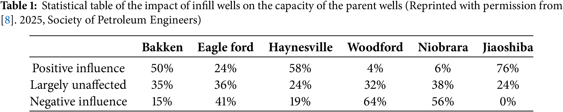
The Changning shale gas region faces challenges including low extraction rates and inadequate reserve utilization as development progresses. Initial shale gas extraction in the Changning area adopted a well spacing of 400–600 m, based on North American development experience. Over 80 horizontal wells with this spacing were drilled before 2017 [1]. However, production data reveal that the average fracture length of horizontal wells is only 100–200 m—less than half the inter-well distance—indicating underutilized reserves between wells. Additionally, the Changning block’s recovery rate of approximately 10% is far below the 20%–50% rates seen in other shale blocks [2,3]. Infill wells have become critical for enhancing shale gas output, but reduced well spacing and pressure depletion zones from parent wells may alter fracture orientations in infill wells [4,5], causing inter-well interference that reduces production efficiency in both wells [6,7]. This poses challenges for quantifying interference between wells and evaluating productivity. Large-scale infill well deployment in U.S. shale gas fields, analyzed through over 3100 interference cases across five North American basins, shows three interference categories: positive, negative, or no effect on parent wells [8,9]. Notably, infill well deployment in China’s Fuling Jiaoshiba block has generally improved parent well performance, as shown in Table 1.
The primary methods for assessing inter-well interference include tracer analysis, production dynamics, and interference well testing [10–12]. While these methods are well-established, few have been applied to evaluate interference from child wells to the parent well. Luo [13] developed linear plots to predict Estimated Ultimate Recovery (EUR) in tight reservoir after infill drilling, categorizing EUR improvements into two mechanisms: enhanced extraction rates and improved recovery in undrained zones. The latter was used to determine optimal infill well spacing. Esquivel and Blasingame [14] analyzed pressure data from 65 parent wells in the Haynesville shale gas field, creating four quantitative metrics and a grading system to measure inter-well connectivity. They also introduced a daily vs. cumulative production plot to assess infill impacts on parent wells but provided only qualitative assessments without quantifying EUR changes. Wang et al. [15] defined three child-parent well distribution models and used machine learning to predict first-year child well production by integrating well location data, fracturing parameters, and production history. However, parent well performance post-infill was not extensively analyzed. Tugan and Weijermars [16] applied a 3-segment decline curve analysis (DCA) to calculate EURs for both parent and child wells, showing high accuracy. However, this method requires substantial production history (4 years for parent wells and 18 months for child wells) are required to ensure reliability.
Huang et al. [17] used numerical simulation to analyze stress shadow effects in multi-stage fractured horizontal wells (MFHWs) in shale reservoirs and their impact on productivity. By integrating hydraulic fracture modeling with reservoir simulation, this study established a workflow to quantify the relationship between fracture interference and well performance. The research identified how key fracturing parameters—including cluster number, stage spacing, and injection rate—control fracture geometry and production outcomes, offering critical insights for optimizing fractures. However, the analysis focused primarily on stress interactions between fracture clusters within a single well and did not examine how fracture-driven interactions in infill well groups affect productivity.
All existing methods only assess the impact of infill wells on parent well EUR qualitatively or calculate EUR for parent or child wells individually, lacking systematic analysis of parent-child well interference and EUR for infill well pats. To address this gap, this study introduces a novel approach: first establishing a multi-well material balance equation with connectivity transmissibility to quantify inter-well flow capacity, then developing a crossflow calculation method to determine infill pad EUR. This work not only addresses the theoretical gap in quantifying inter-well interference but also provides critical foundations for accurate EUR prediction and development optimization in shale oil/gas infill drilling. Additionally, it offers actionable insights to improve unconventional reservoir development efficiency.
2 Impact of Shale Gas Child Wells Infill on Parent Wells
The Changning shale gas infill pilot test platform CN1 includes three parent wells (CN1, CN2, CN3) spaced 500 m apart, each with a horizontal section length of 1500–1800 m. These wells were commissioned in 2015. Prior to infill drilling, the parent wells had an average cumulative production exceeding 0.86 × 10⁸ m3. In 2022, two infill wells (CN4 and CN 5) were drilled between the parent wells at a spacing of 250 m. Their horizontal sections measure 1601 and 1803 m, respectively, with the vertical wellbore trajectory offset 8 m from the parent wells. The platform layout is shown in Fig. 1. The thicknesses of Layers 1, 2, 3, and 4 are 0.9, 7.9, 7.5, and 24.3 m, respectively. The horizontal sections of parent wells CN1–CN3 are located between Layers 3 and 4, while infill wells CN4-CN5 are between Layers 1 and 2.
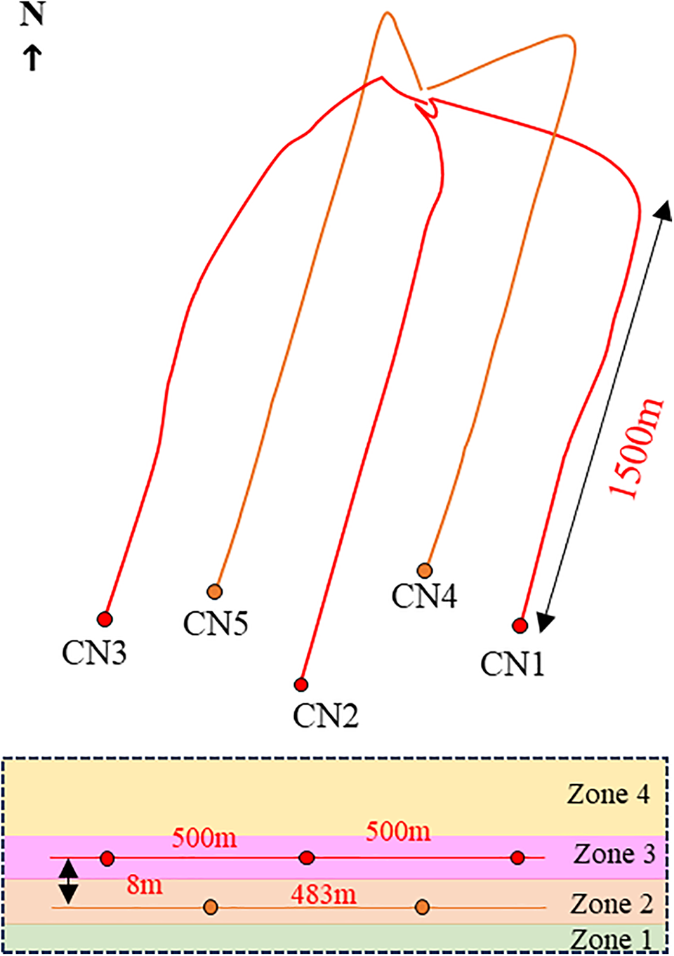
Figure 1: Schematic of CN1 platform well location
2.1 Wellhead Pressure Monitoring during Fracturing
Inter-well interference occurs throughout gas well production. During infill well fracturing, pressure changes in offset wells reflects the degree of hydraulic fractures interference. Stronger fracturing-induced interference correlates with higher wellhead pressure increases, while weaker interference causes smaller fluctuations. The cumulative pressure increases per stage in each well quantifies interference intensity between the monitored and fracturing wells. Additionally, the ratio of each stage’s pressure increase to the total cumulative represents the relative contribution of individual fracturing stages [18].
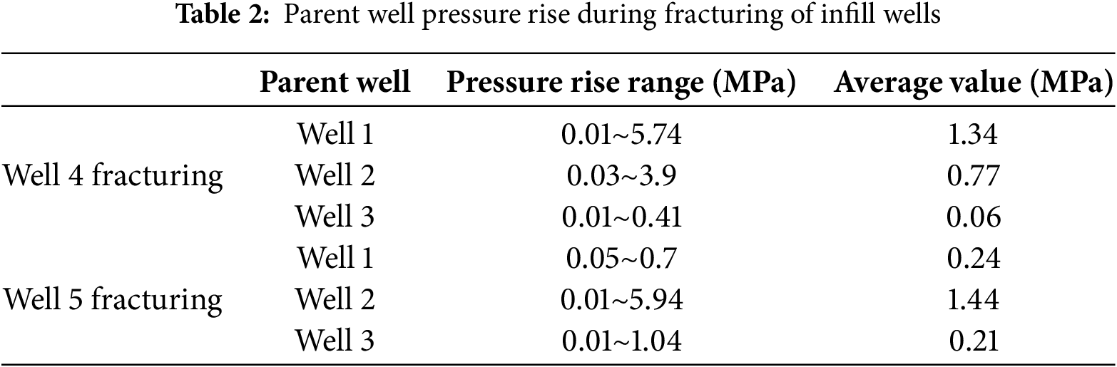
The wellhead pressure rise of the parent well was monitored during the fracturing of the infill, and the results are shown in Figs. 2 and 3. Well 4 fractured 21 segments, the pressure of well 1 responded to 13 segments with a pressure increase of 0.01~5.71 MPa, well 2 responded to 15 segments with a pressure increase of 0.03~3.9 MPa, and well 3 responded to 13 segments with a pressure increase of 0.01~0.41 MPa during the fracturing period. Well 5 was fractured in 23 sections, the pressure response of well 1 was 8 sections with a pressure increase of 0.05~0.7 MPa, the pressure response of well 2 was 19 sections with a pressure increase of 0.01~0.5.94 MPa, and the pressure response of well 3 was 13 sections with a pressure increase of 0.01~1.04 MPa during the fracturing period, the results are shown in Table 2.
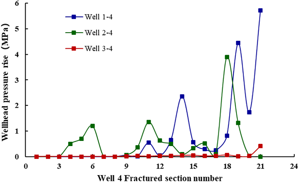
Figure 2: Well 4 wellhead pressure rise in parent wells during fracturing
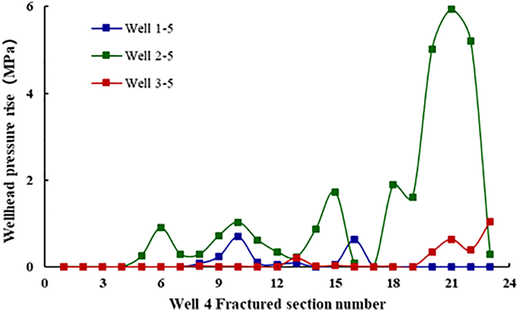
Figure 3: Well 5 wellhead pressure rise in parent wells during fracturing
The wellhead pressure increases in monitoring wells were calculated using the fracturing timeline of each infill well stage (Tables 3 and 4). Using Well 4 as a case study. Well 1 recorded a total pressure rise of 17.47 MPa during Well 4’s fracturing, with notably high spikes in Stages 14, 19, 20 and 21 (13.51%, 25.42% and 32.68%, respectively), indicating strong fracture-driven interference. Well 2 displayed a total increase of 11.57 MPa, with higher responses (>10%) in Stages 6, 11, 18 and 19, demonstrating substantial interference. Well 3 experienced only a minor rise of 0.74 MPa, suggesting weak interference with Well 4.
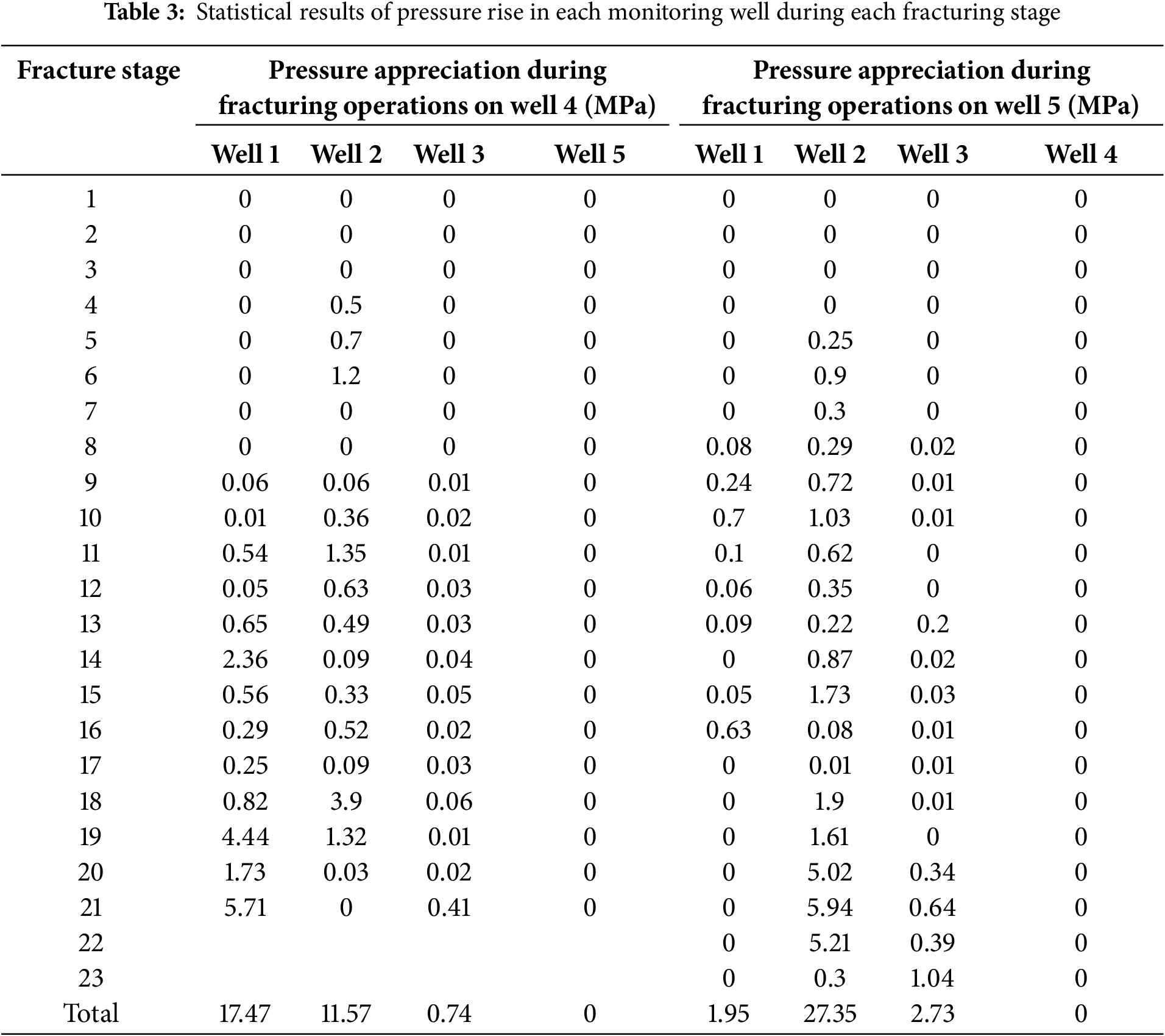
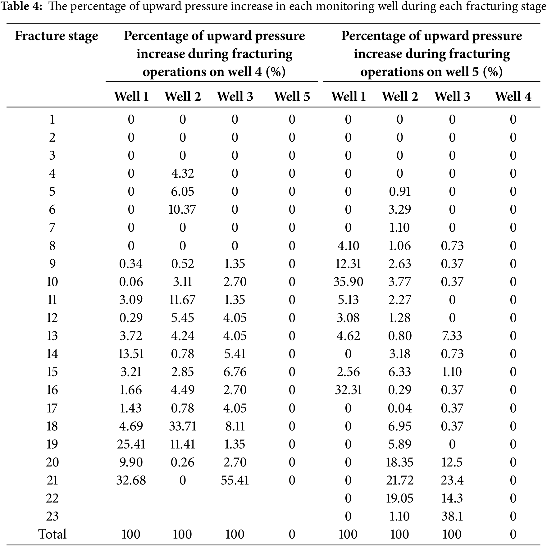
During Well 5’s hydraulic fracturing, cumulative pressure increases were 1.95 MPa (Well 1), 27.35 MPa (Well 2), and 2.73 MPa (Well 3), with strongest interference between Wells 2 and 5 (Stages 20–22: 18.35%, 21.72%, 19.05%). Well positioning significantly influenced pressure responses: closer distances correlated with stronger interference, while no fracturing response was observed between infill Wells 4 and 5.
2.2 Tracer Monitoring during the Flowback Phase
In fracture networks with large cracks, tracer output displays a sharp, narrow single-peak curve. In systems dominated by microfractures, the curve shows a short, broad single or multi-peak pattern, where the peak count depends on the number of high-permeability channels [19,20]. Therefore, fracture connectivity can be determined by analyzing tracer curve shapes, as illustrated in Fig. 4.
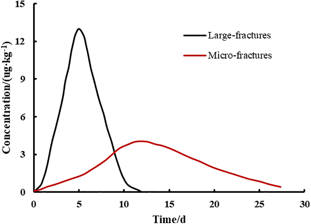
Figure 4: Schematic tracer flowback curve
A fracturing fluid, containing 44 gas-phase tracers was injected via infill wells CN4 and CN5. Subsequent to the opening of the wells, varying concentrations of tracers were observed in all three parent wells, with concentration curves illustrated in Fig. 5. Wells 1 and 2 (from Well 4) and Well 2 (from Well 5) showed elevated tracer concentrations with double peaks, indicating connectivity through large fractures. Well 3 exhibited low concentrations with a single late peak, suggesting microfracture-dominated connectivity. Wells 3 and 5 did not detect tracer injection from well 4, whereas wells 1 and 4 did not detect tracer injection from well 5. Cross-well tracer monitoring showed no mutual tracer detection between Wells 4 and 5. Peak intensity and curve width analysis revealed stronger connectivity in well pairs 1–4, 2–4, and 2–5 compared to 3–5.
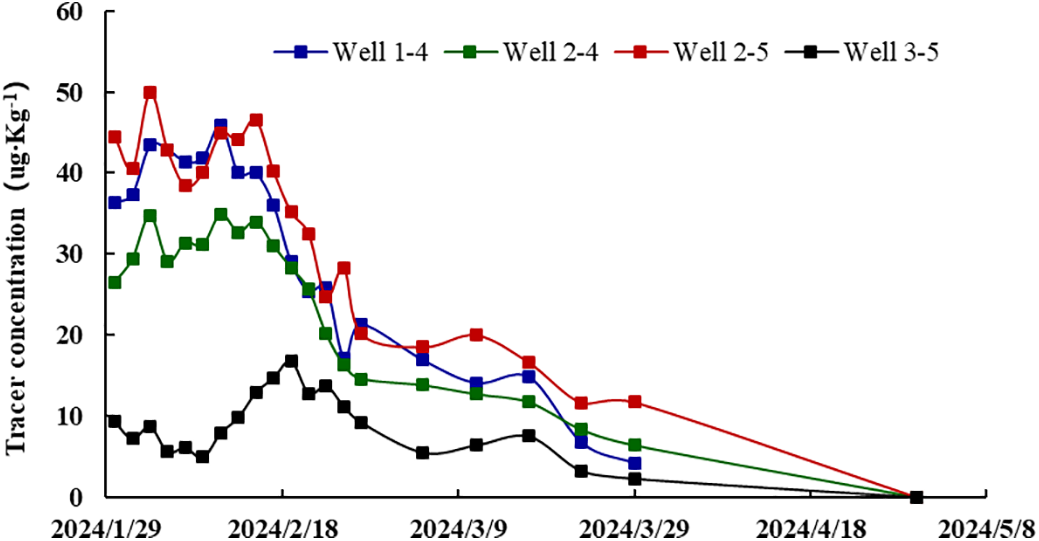
Figure 5: CN1 platform tracer monitoring concentration curves
As shown in Fig. 6, tracer concentrations peaked then declined. By the final monitoring stage, concentration in multiple wells dropped to undetectable levels, signifying that fractures between infill and parent wells gradually closed under stress, reducing inter-well flow.
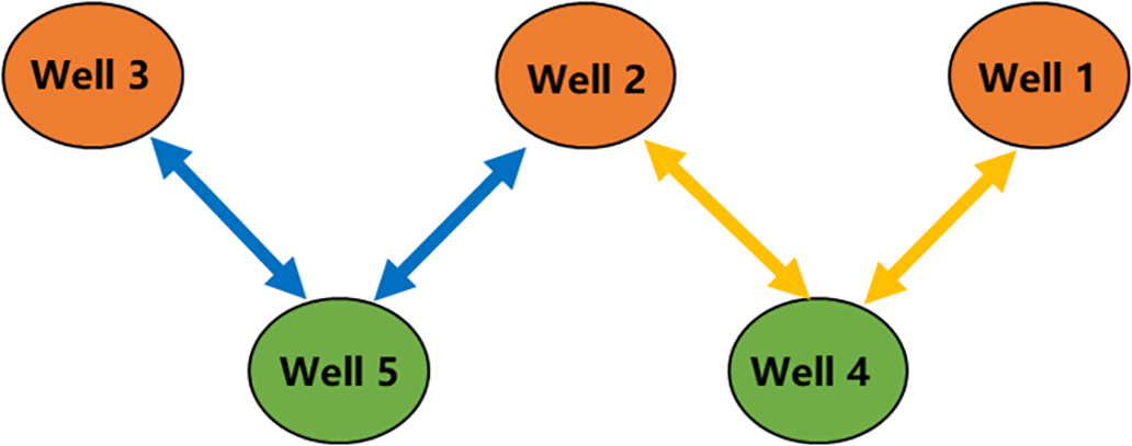
Figure 6: Tracer monitoring shows the connectivity of infill to parent wells
Fig. 7 shows the spatial distribution of micro-seismic monitoring results for Platform CN1. Green dots denote the parent well events, while purple dots denote child well events. Both color-coded event clusters are symmetrically distributed along the wellbore. Prior to infill drilling, micro-seismic events between parent wells were sparsely distributed. Following infill operations, the micro-seismic events between parent and child wells demonstrate uniform spatial coverage across the entire pad. Additionally, micro-seismic data from this platform indicate a well-defined natural fracture network connecting wells 1, 2, 4, and 5. This fracture system is marked by clustered micro-seismic events, consistent with tracer detection results.
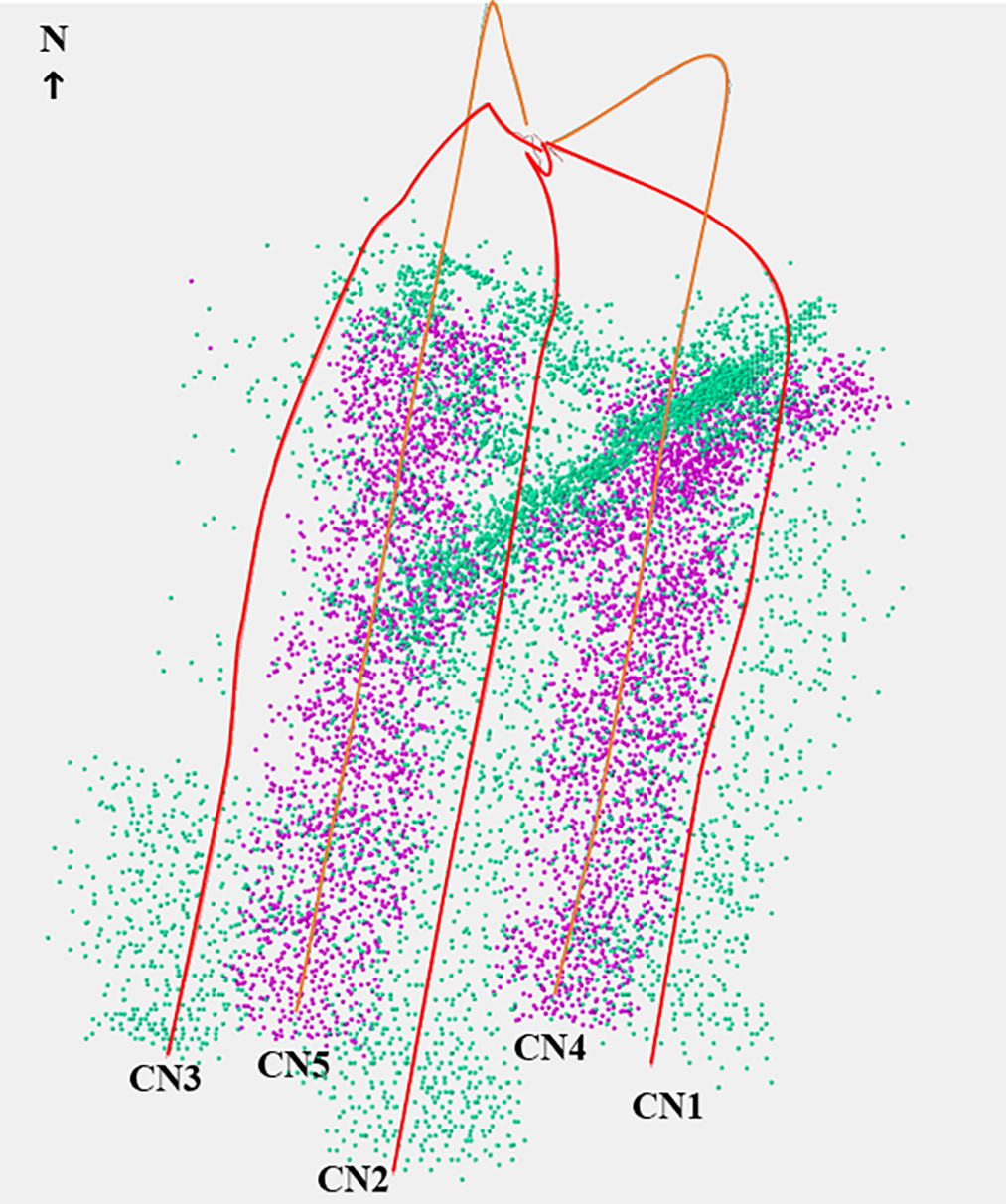
Figure 7: CN1 platform micro-seismic event points
2.3 Analysis of Interference Well Test in the Early Stage of Production
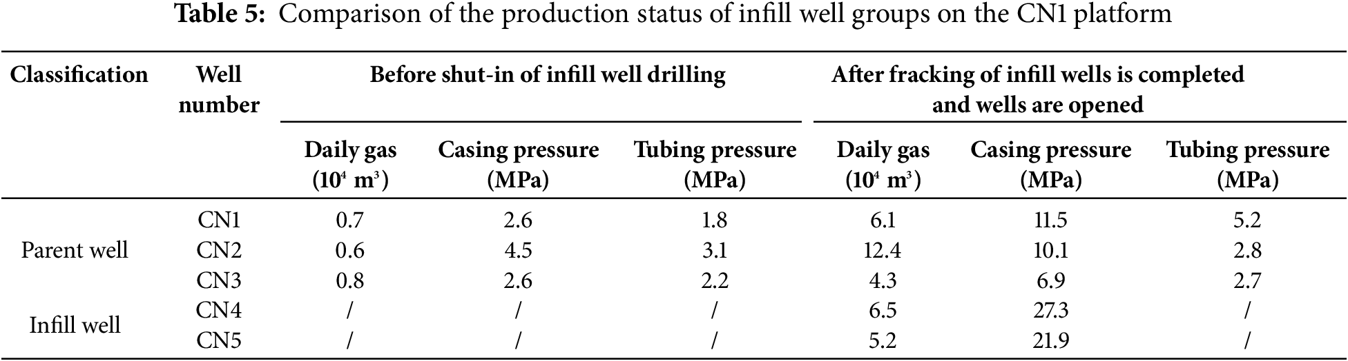
In January 2023, five wells commenced production. Post-infill reopening of parent wells resulted in higher initial output compared to pre-infill levels (Table 5).
To verify the inter-well connectivity, an interference test was conducted on the platform in April 2023. Two wells between Wells 4 and 5 remained open during the test due to partially closed wellhead gates. Wells CN1, CN4, and CN5 were selected as test wells to evaluate connectivity by analyzing pressure fluctuation timing and patterns in observation wells [21]. The distance from well CN1 to 4 is 251 m, and the results of the interference test for the well CN1 and 4 groups are illustrated in Fig. 8. The CN4 well exhibited an opening pressure excitation response time [22] of 1.8 h, a propagation speed of 139 m per hour, an excitation duration of 307.87 h, and a pressure drop of 1.79 MPa. The CN4 well exhibited a shut-in excitation reaction time of 2.67 h, a propagation velocity of 94 m per hour, an excitation duration of 122.62 h, and a pressure increase of 1.29 MPa.
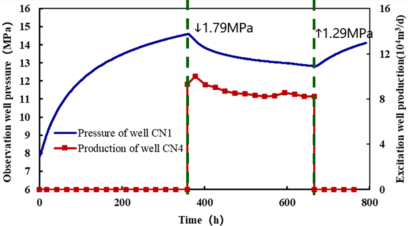
Figure 8: CN1 well pressure response during CN4 well excitation
The distance from CN4 to well 5 was 483 m, and the results of the interference test for the CN4 and well 5 groups are illustrated in Fig. 9. The reaction time for the CN4 well shut-in excitation is 10.43 h, the propagation speed is 46 m per hour, the excitation duration is 112.55 h, and the pressure increase is 0.17 MPa.
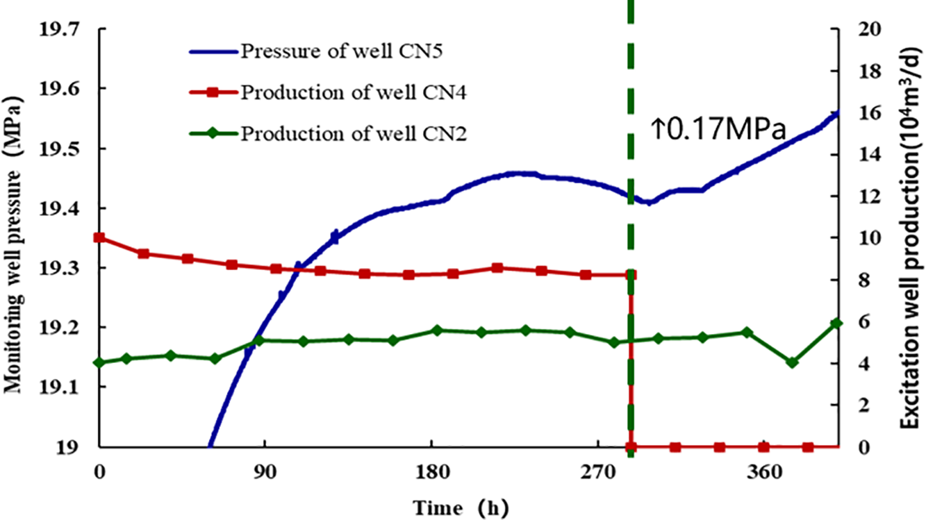
Figure 9: CN5 well pressure response during CN4 well excitation
The interference test findings indicate that wells CN1 and CN4 demonstrate connectivity through propped fractures. With a spacing of 483 m between Wells CN4 and CN5, pressure interference is evident, confirming that infill wells establish hydraulic connectivity with parent wells. This connectivity provides pressure support, enhancing parent well productivity during early production phases.
During fracturing, flowback, and production operations, child wells induce notable interference on parent wells. As child well pressure declines, fracture connectivity initially remains high but gradually decreases due to stress-induced fracture closure. Therefore, quantifying transient flow rates between parent and infill wells is critical for accurate EUR evaluation of infill wells.
3 Calculation of Crossflow between Child Wells and Parent Wells Considering Desorption Action
3.1 Material Balance Equation for an Infill Well Group
Assumptions in this study:
1. Pre-infilling conditions:
-The parent wells, comprising a total of n wells, had been in production for several years prior to the deployment of infill wells.
- No connectivity was observed between of the any parent wells during this period. Therefore, we assume that the parent wells operated as independent systems before infill well activation.
2.Post-infilling conditions:
- When infill wells begin production, communication develops between the infill and parent wells.
- This communication induces pressure differentials attributable to variations in remaining reserves and disparities in cumulative gas production per well [23].
- The variations in pressure create conductive pathways between wells, thereby establishing a replenishment relationship between wells.
3.Connectivity constraints:
- Only adjacent wells demonstrate connectivity.
- Non-adjacent wells remain non-connected.
4.Shale-specific considerations:
- The model accounts for adsorbed/desorbed gas volumes from shale formations.
A schematic diagram of the connectivity of the infill well to the parent well is shown in Fig. 10.
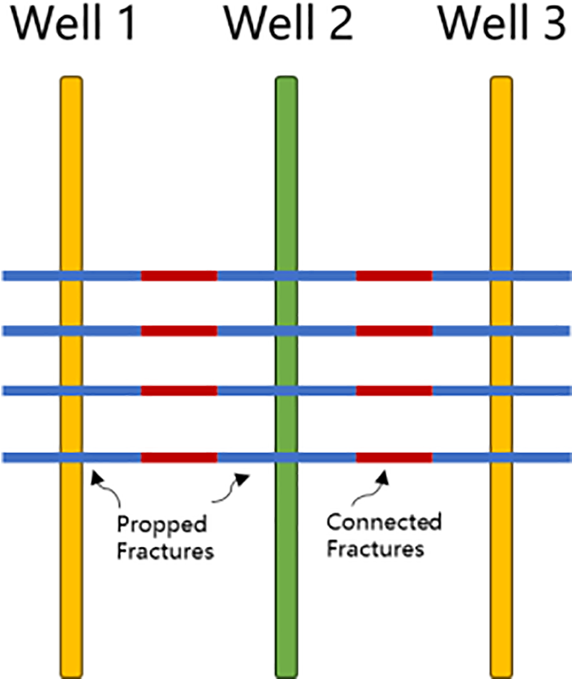
Figure 10: Schematic diagram of inter-well connectivity of the infill platform. (where: wells 1 and 3 are parent wells, and well 2 is infill well, connectivity between infill wells and parent wells is achieved through connected fractures)
Shale gas reservoirs contain both free gas and adsorbed gas. Free gas is stored in fractures and matrix pores, while adsorbed gas is bound to the internal surfaces of the matrix [24]. During production, reservoir pressure declines. When the pressure falls below the critical desorption threshold, adsorbed gas begins to desorb. Assuming t isothermal reservoir conditions, the Langmuir adsorption isotherm equation is used to derive the material balance equation [25,26], namely:
VL represents the Langmuir volume, indicating the maximum theoretical saturated adsorption capacity of shale when formation pressure approaches infinity. PL denotes the Langmuir pressure, corresponding to the pressure at which 50% of gas adsorption capacity is achieved on the Langmuir isotherm curve. A lower Langmuir pressure indicates that adsorbed gas is less prone to desorption during production.
Under conditions of initial formation pressure, denoted as pi, the reserves of shale gas comprise the total amount of both free and adsorbed gas, specifically:
Based on the principle of mass conservation (ρ1V1 = ρ2V2), the original subsurface adsorbed gas volume in the adsorbed phase can be calculated as:
Assuming constant densities for both the adsorbed gas phase and free gas phase, the volume of the remaining subsurface adsorption gas adsorption term volume is expressed as follows:
When the formation pressure drops, the volume of expansion of the rock with bound water is:
As the formation pressure diminishes and a portion of the free-state adsorbed gas is extracted, the volume of the remaining free-state adsorbed gas in the subsurface is:
According to the principle of subsurface volume equilibrium can be obtained:
Original free gas volume + Original adsorbed gas volume = Remaining free gas volume + Remaining adsorbed gas desorption volume + Remaining adsorbed gas adsorption term volume + Rock and bound water expansion volume
Setting
By bringing Eq. (8) into Eq. (7) and dividing both sides by GBgi at the same time:
Setting Enhanced gas deviation factor:
The material balance equation, which accounts for adsorption-desorption processes and inter-well connectivity, is as follows:
From Eq. (11), Accounting for adjacent well interference exhibiting sequential j − 1 → j → j + 1 chained conductivity, the material balance equation for the j well (1 < j < n) is:
In Eq. (12): Gj(j+1) and G(j−1)j are the cumulative gas flurries from well j to well j + 1 and from well j − 1 to well j, respectively, at a given time, 108 m3. In this paper, it is assumed that well j crossflow to well j + 1, and j − 1 crossflow to well j. The amount of crossflow between well j and a non-adjacent well is zero.
The material balance equation of the 1st well is:
The material balance equation for the n-th well is:
Eq. (11) is the material balance equation for shale gas wells, which accounts for adsorption, desorption, and inter-well connectivity. To facilitate the crossflow calculation, this study employed the methodology outlined in reference [27] for the solution.
When the reserves are known, Eqs. (12)–(14) are actually functions about the pressure of each well, then Eqs. (12)–(14) are rewritten as:
For the calculation of gas crossflow from well j to well k at a given time in Eq. (12), we assume Darcy’s law applies, resulting in the following equation:
There is:
Setting:
Then it is obtained from Eq. (10):
The pseudo-pressures for Well j and Well k are respectively defined as:
Then:
To quantitatively characterize the connectivity between Well j and Well k, connected conductivity:
Since the accurate acquisition of average permeability and the contact area between wells is practically challenging, the introduction of connectivity transmissibility avoids potential errors from the direct calculation.
Then Eq. (24) can be rewritten as:
At the moment t + Δt, the cumulative gas crossflow from well j to well k is solved using the iterative step-by-step method, which is calculated as:
Substituting Eq. (24) into Eq. (25) obtains:
To ascertain the formation pressure of each well at any given moment and the volume of inter-well crossflow, the Newton-Raphson iterative method for nonlinear systems of equations was employed in conjunction with the established material balance calculation model for a well group. The calculation formula is as follows:
In Eq. (29), l is the number of iterations. According to Eq. (29), the nonlinear iterative matrix equation can be constructed:
The formula for each variable in the Jacobi coefficient matrix on the left-hand side of Eq. (30) is:
Connectivity exists between neighboring wells, then:
No connectivity between non-adjacent wells:
According to Eqs. (31)–(33), it can be seen that the constructed Jacobi iteration coefficient matrix is a tridiagonal coefficient matrix. Therefore, the pressure of each well at each time step can be solved by Eq. (30).
3.2 Calculation and Validation of Crossflow from Child Wells to Parent Wells in an Infill Well Group
Formation pressure and crossflow in the CN1 platform infill well group were determined using the methodology from Section 3.1. Initial parent and child well pressures were derived from Diagnostic Fracture Injection Testing (DFIT), and initial reserves were estimated via declining production analysis. Inter-well conductivity was initialized using Eq. (25). The model computed formation pressure at discrete time steps, iteratively updating conductivity and crossflow values based on pressure build-up data. Results are shown in Fig. 11.
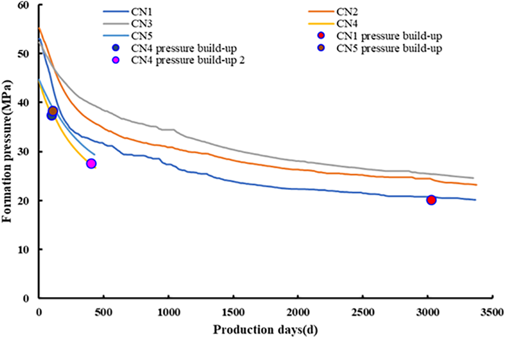
Figure 11: CN1 platform formation pressure calculation results
Fig. 11 indicates strong agreement between simulated and measured pressures, validating the model’s reliability. After infill drilling, the child well’s initial pressure was lower than the parent well. However, prolonged parent well production prior to child well activation caused reservoir pressure decline. Consequently, child well pressure exceeded parent well pressure during activation, triggering crossflow.
To validate the computational accuracy, this study uses the Rate Transient Analysis (RTA) module in IHS Harmony™ [28] to simulate parent well formation pressure before infill drilling (pr-2700 days in Fig. 11). A comparison between our method and RTA results (Fig. 12) shows consistent pressure trends and numerical alignment, with a mean relative error <5%, confirming the method’s reliability for single-well pressure prediction.
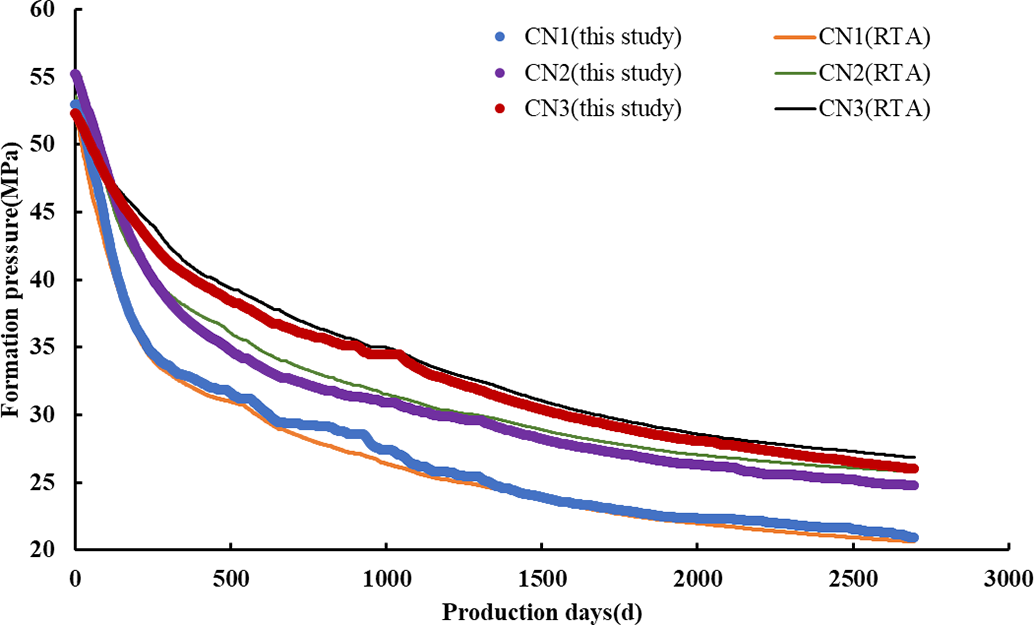
Figure 12: CN1 platform formation pressure calculation results
However, after child well activation (i.e., post-fracturing), the original single-well model fails to accurately predict pressures due to hydraulic connectivity between parent and child wells via engineered fractures. Post-infill pressure calculations therefore rely on measured formation pressure data (Fig. 11).
Figs. 13 and 14 calculate the instantaneous and cumulative crossflows from each child well to the parent well, respectively. Well 4 had 471 × 104 m3 of crossflow to well 1 and 579 × 104 m3 of crossflow to well 2. Well 5 had 433 × 104 m3 of crossflow to well 2 and 313 × 104 m3 of crossflow to well 3.
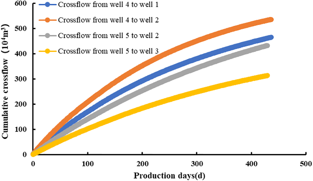
Figure 13: Results of CN1 platform cumulative inter-well crossflow calculations
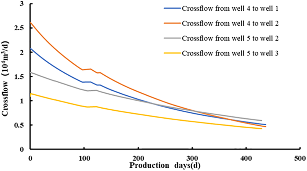
Figure 14: Instantaneous crossflow from child wells to parent wells
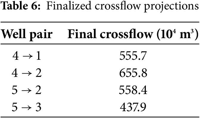
As production continues, child well pressure declines, reducing the pressure differential between child and parent wells. Consequently, instantaneous crossflow to the parent well gradually decreases. The study defines negligible crossflow as instantaneous values below 10% of the parent well’s pre-infill production rate. Using this threshold, the cumulative crossflow volume from child to parent wells—equivalent to the parent well’s EUR increment post-infill—was calculated (Table 6).
4 Evaluation of Infill Wells EUR
4.1 Diagnosis of Analytical Modeling of Diminishing Production in Infill Wells
EUR can be estimated via the Rate Transient Analysis (RTA) method once a gas well reaches boundary-dominated flow (BDF). Shale gas wells typically require years of linear flow before achieving BDF [29,30]. Diagnostic plots for Wells CN4 and CN5 (Figs. 15 and 16) confirm both wells have entered BDF due to inter-well interference: infill well production propagates into parent well depletion zones, accelerating BDF onset. The multi-stage fractured horizontal well model was applied to calculate EUR. Results show simulated EURs for Wells CN4 and 5 are 0.78 × 10⁸ m3 and 0.85 × 10⁸ m3, respectively.
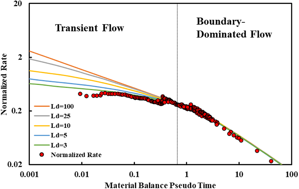
Figure 15: CN4 well characterization curve determination
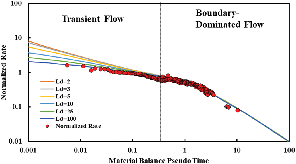
Figure 16: CN5 well characterization curve determination
4.2 EUR Calculation for Infill Well Platforms
The EUR for the CN1 platform can be ascertained once it is confirmed that shale gas infill wells are suitable for EUR calculations using the horizontal well multi-stage fracturing analytical model. Additionally, parent wells can be employed to compute post-infill EUR by adding the pre-infill calculated EUR to the total crossflow volume. Table 7 presents the EUR calculations for the parent wells both prior to and following infill.
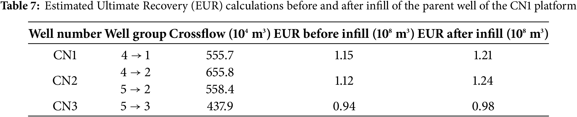
Post-infill analysis reveals EUR increments of 0.04~0.12 × 10⁸ m3 across three parent wells, cumulatively reaching 0.22 × 10⁸ m3. The CN2 well is located between the two child wells and obtains recharge from the two infill wells, with the largest incremental increase in EUR. The total EUR of the two infill wells is 1.63 × 10⁸ m3 and adding the increased EUR of the parent well, the EUR of the infill platform increases by 1.85 × 10⁸ m3.
This study introduces an innovative technical approach for the development of shale gas through the formation of a multi-well material balance equation and a quantitative method for calculating inter-well crossflow. By incorporating the connectivity transmissibility parameter (Eq. (25)), this methodology facilitates the quantitative evaluation of inter-well interference effects, thereby offering a more precise assessment of production performance for infill well pads. Practically, this novel approach provides a theoretical basis for optimizing production designs and adjusting fracturing strategies in shale gas reservoirs, ultimately improving development efficiency. Future research will further explore the effects of well spacing and fracturing parameters on the productivity of infill well groups, based on these findings, to achieve higher recovery rates.
1. Various monitoring techniques employed during the fracturing, flowback, and production phases have revealed inter-well interference between the infill and parent wells subsequent to the establishment of the infill wells. The interference response of the parent well situated between two infill wells was more pronounced than that of the parent well located adjacent to only one infill well.
2. This study formulates a multi-well material balance equation that integrates the processes of shale gas adsorption and desorption. This formulation facilitates the determination of formation pressure and allows for the quantitative evaluation of inter-well crossflow.
3. Child wells exhibit boundary flow characteristics that enable the estimation of EUR through a multi-stage fracturing analytical model for horizontal wells. The parent well EUR is the EUR prior to infill plus the total cumulative infill crossflow.
Acknowledgement: Not applicable.
Funding Statement: The authors received no specific funding for this study.
Author Contributions: The authors confirm contribution to the paper as follows: Conceptualization, Cuiping Yuan; methodology, Sicun Zhong; software, Cuiping Yuan; validation, Jia Chen; formal analysis, Ying Wang; investigation, Yinping Cao; resources, Yijia Wu, Man Chen; data curation, Yinping Cao; writing—original draft preparation, Cuiping Yuan; writing—review and editing, Sicun Zhong, Yijia Wu; supervision, Sicun Zhong. All authors reviewed the results and approved the final version of the manuscript.
Availability of Data and Materials: The data that support the findings of this study are available from the corresponding author upon reasonable request.
Ethics Approval: Not applicable.
Conflicts of Interest: The authors declare no conflicts of interest to report regarding the present study.
Nomenclature
| pi | Original formation pressure of the gas reservoir (MPa) |
| VE | Isothermal adsorption at the pressure p (m3·m−3) |
| VL | Langmuir’s volume (m3·m−3) |
| pL | Langmuir’s pressure (MPa) |
| p | Formation pressure (MPa) |
| G | Geologic reserves of the gas reservoir (108 m3) |
| Gp | Cumulative gas production (108 m3) |
| Gv | Amount of runoff from the neighboring well to this well (108 m3) |
| Gk | Amount of runoff from this well to the neighboring well (108 m3) |
| Gf | Geologic reserves of free gas (108 m3) |
| Ga | Geologic reserves of adsorbed gas (108 m3) |
| φ | Porosity (fraction) |
| Sgi | Gas saturation of the original free gas (fraction) |
| Swi | Initial water saturation (fraction) |
| Bgi | The original gas volume factor (m3·m−3) |
| Bg | Gas reservoir volume factor, pressure-dependent (m3·m−3) |
| μg | Viscosity, pressure-dependent (mPa·s) |
| ρB | Rock density (g·cm−3) |
| Cf | Rock compressibility (MPa−1) |
| Cw | Water compressibility (MPa−1) |
| Gais | Volume of the adsorbed gas at a formation pressure of pi (108 m3) |
| Gas | Volume of the adsorbed gas at a formation pressure of p (108 m3) |
| ΔVep | Sum of the altered volumes of rock and irreducible water (108 m3) |
| ΔVed | Remaining free-state adsorbed gas in the subsurface (108 m3) |
| zi | Original gas deviation coefficient |
| z | Gas deviation factor when the pressure is p |
| z* | Enhanced gas deviation factor |
| zi* | Enhanced gas deviation factor in original condition |
| zj* | Enhanced gas deviation factor of the well j |
| pj | Pressure at a certain moment in well j (MPa) |
| pk | Pressure at a certain moment in well k (MPa) |
| Gj | Geologic reserves of the well j (108 m3) |
| Gpj | Cumulative gas production of the well j (108 m3) |
| Gj(j+1) | Cumulative crossflow at a certain moment from well j to well j + 1 (108 m3) |
| G(j−1)j | Cumulative crossflow at a certain moment from well j − 1 to well j (108 m3) |
| Gjk | Cumulative crossflow at a certain moment from well j to well k (108 m3) |
| Fj | Pressure-dependent function |
| qjk | Gas channeling velocity between wells j and k (m3·d−1) |
| kjk | Seepage channel permeability between wells j and k (10−3 μm2) |
| Ajk | Cross-sectional area between wells j and k (m2) |
| Ljk | Distance between wells j and k |
| α | Unit conversion factor 0.0864 |
| T | Temperature (K) |
| psc | Standardized gas reservoir pressure 0.101 MPa |
| Tsc | Standardized gas reservoir temperature 298.15 K |
| mj | Pseudo-pressure for wells j (MPa) |
| mk | Pseudo-pressure for wells k (MPa) |
| t | Time (d) |
| Δt | Time increment |
References
1. Zhao SS, Xia ZQ, Zheng MJ, Zhang DL, Liu SJ, Liu YY, et al. Evaluation of the remaining reserves of shale gas and countermeasures to increase the utilization of reserves: case study of the Wufeng-Longmaxi formations in Changning area, southern Sichuan Basin. J Nat Gas Geosci. 2023;34(8):1401–11. (In Chinese). doi:10.1016/j.jnggs.2023.11.002. [Google Scholar] [CrossRef]
2. Baihly JD, Altman RM, Malpani R, Luo F. Shale gas production decline trend comparison over time and basins. In: The SPE Annual Technical Conference and Exhibition; 2010 Sep 19–22; Florence, Italy. p. 1–25. doi:10.2118/135555-ms. [Google Scholar] [PubMed] [CrossRef]
3. Thorkelson J, Fox P, Kulkarni MM, Jensen T. Data driven Woodford Shale risk characterization. In: The SPE/AAPG/SEG Unconventional Resources Technology Conference; 2013 Aug 12–14; Denver, CO, USA. 1229 p. doi:10.1190/urtec2013-243. [Google Scholar] [CrossRef]
4. Mukherjee H, Poe BD, Heidt JH, Watson TB, Barree RD. Effect of pressure depletion on fracture-geometry evolution and production performance. SPE Prod & Fac. 2000;15(3):144–50. doi:10.2118/30481-ms. [Google Scholar] [PubMed] [CrossRef]
5. King GE, Rainbolt MF, Swanson C. Frac hit induced production losses: evaluating root causes, damage location, possible prevention methods and success of remedial treatments. In: Proceedings of the SPE Annual Technical Conference and Exhibition; 2017 Oct 9–11; San Antonio, TX, USA. 44 p. doi:10.2118/187192-MS. [Google Scholar] [PubMed] [CrossRef]
6. Alzahabi A, Kamel A, Harouaka A, Trindade AA. A model for estimating optimal spacing of the Wolfcamp in the Delaware Basin. In: Proceedings of the 8th Unconventional Resources Technology Conference; 2020 Jul 20–22; Austin, TX, USA. doi:10.15530/urtec-2020-2645. [Google Scholar] [CrossRef]
7. Crespo P, Pellicer M, Crovetto C, Gait J. Quantifying the parent-child effect in Vaca Muerta Formation. In: Proceedings of the 8th Unconventional Resources Technology Conference; 2020 Jul 20–22; Austin, TX, USA. doi:10.15530/urtec-2020-1035. [Google Scholar] [CrossRef]
8. Grant M, Garrett L, Jason B, Xu T. Parent well refracturing: economic safety nets in an uneconomic market. In: The SPE Low Perm Symposium; 2016 May 5–6; Denver, CO, USA. p. 1–15. doi:10.2118/180200-ms. [Google Scholar] [PubMed] [CrossRef]
9. Gupta I, Rai C, Devegowda D, Sondergeld C. A data-driven approach to detect and quantify the impact of frac-hits on parent and child wells in unconventional formations. In: The Unconventional Resources Technology Conference; 2020 Jul 20–22; Austin, TX, USA. doi:10.15530/urtec-2020-2190. [Google Scholar] [CrossRef]
10. Chu WC, Kyle DS, Ray F, Chen C, Michael DZ. A new technique for quantifying pressure interference in fractured horizontal shale wells. SPE Res Eval Eng. 2020;23(1):143–57. doi:10.2118/191407-pa. [Google Scholar] [PubMed] [CrossRef]
11. Ilkay U, Wisam A, Erdinc E. Application of Well interference test using distributed pressure sensors to optimize well spacing in unconventional shale reservoirs. In: The Abu Dhabi International Petroleum Exhibition & Conference; 2019 Nov 11–14; Abu Dhabi, United Arab Emirates. p. 1–16. doi:10.2118/197936-ms. [Google Scholar] [PubMed] [CrossRef]
12. Qin J, Cheng S, Zhu J. Integrated approach for well interference diagnosis considering complex fracture networks combining pressure and rate transient analysis. In: The SPE Annual Technical Conference & Exhibition; 2020 Oct 26–29; Denver, CO, USA. p. 1–25. doi:10.2118/201284-ms. [Google Scholar] [PubMed] [CrossRef]
13. Luo S, Kelkar M. Infill-drilling potential in tight gas reservoirs. J Energy Resour Technol. 2013;135(1):013401. doi:10.1115/1.4007662. [Google Scholar] [CrossRef]
14. Esquivel R, Blasingame T. Optimizing the development of the Haynesville Shale—lessons learned from well-to-well hydraulic fracture interference. In: Proceedings of the 5th Unconventional Resources Technology Conference; 2017 Jul 24–26; Austin, TX, USA. p. 1–22. doi:10.15530/urtec-2017-2670079. [Google Scholar] [CrossRef]
15. Wang H, Chen Z, Chen SN, Hui G, Kong B. Production forecast and optimization for parent-child well pattern in unconventional reservoirs. J Pet Sci Eng. 2021;203:108899. doi:10.1016/j.petrol.2021.108899. [Google Scholar] [CrossRef]
16. Tugan MF, Weijermars R. Improved EUR prediction for multi-fractured hydrocarbon wells based on 3-segment DCA: implications for production forecasting of parent and child wells. Amsterdam, The Netherlands: Elsevier; 2020. doi:10.1016/j.petrol.2019.106692. [Google Scholar] [CrossRef]
17. Huang L, Jiang P, Zhao XY, Yang L, Lin JY, Guo XY. A modeling study of the productivity of horizontal wells in hydrocarbon-bearing reservoirs: effects of fracturing interference. Geofluids. 2021;2021(1):2168622. doi:10.1155/2021/2168622. [Google Scholar] [CrossRef]
18. Liu L, Tang YW, Zheng AW, Zhang Q, Wang YM, Cai J. New approach of evaluating fracturing interference based on wellhead pressure monitoring data: a case study from the well group-A of Fuling shale gas field. J Pet Explor Prod Technol. 2024;14(1):139–48. doi:10.1007/s13202-023-01713-3. [Google Scholar] [CrossRef]
19. Liu WD, Liu TJ, Ji YJ, Zhang LF, Chu FD, Zhang L. Determination of inter-well connectivity of fractured fractures in glutenite reservoirs by micro-seismic monitoring results: a case study of Mahu Oilfield in the Junggar Basin. Oil Geophys Prospect. 2022;57(2):395–404. (ln Chinese). doi:10.27643/d.cnki.gsybu.2018.000167. [Google Scholar] [CrossRef]
20. Du DF, Hao FH, Li Y, Li D, Tang YJ. Study on interpretation method of multistage fracture tracer flowback curve in tight oil reservoirs. ACS Omega. 2024;9(10):11628–36. doi:10.1021/acsomega.3c08411. [Google Scholar] [PubMed] [CrossRef]
21. Qiu ZY, Xie D, Pu YL, Gao ZW, Guo R. Research on connectivity of extra-low porosity and permeability fracture-pore type glutenite oil reservoir in interference well test way—a case study of the area of Well Hong153 in Junggar Basin. Sino-Glob Energy. 2019;24:40–6.(ln Chinese). [Google Scholar]
22. Kumar A, Seth P, Shrivastava K, Manchanda R, Sharma M. Integrated analysis of tracer and pressure-interference tests to identify well interference. SPE J. 2020;25:1623–35. doi:10.2118/201233-pa. [Google Scholar] [PubMed] [CrossRef]
23. Weijermars R, Tugan MF, Khanal A. Production rates and EUR forecasts for interfering parent-parent wells and parent-child wells: fast analytical solutions and validation with numerical reservoir simulators. J Pet Sci Eng. 2020;190(3):107032. doi:10.1016/j.petrol.2020.107032. [Google Scholar] [CrossRef]
24. Abdel AR, Aljehani A, Alatefi S. Estimation of free and adsorbed gas volumes in shale gas reservoirs under a poro-elastic environment. Energies. 2023;16(15):5798. doi:10.3390/en16155798. [Google Scholar] [CrossRef]
25. Shi JT, Jia YR, Zhang LL, Ji CJ, Li GF, Xiong YX, et al. The generalized method for estimating reserves of shale gas and coalbed methane reservoirs based on material balance equation. Pet Sci. 2022;19(6):2867–78. doi:10.1016/j.ptesci.2022.07009. [Google Scholar] [CrossRef]
26. Abdel AR, Alatefi S, Alkouh A. Estimation of shale gas reserves: a modified material balance equation and numerical simulation study. Processes. 2023;11(6):1746. doi:10.3390/pr11061746. [Google Scholar] [CrossRef]
27. Meng FK, Liu XH, Guo ZH, Luo RL, Liu J. Evaluation on inter-well groups connectivity with material balance equation (MBE) for heterogeneous gas reservoirs. Nat Gas Geosci. 2023;35:1070–81. (In Chinese). doi:10.11764/j.issn.1672-1926.2023.10.021. [Google Scholar] [CrossRef]
28. Quintero G. Quantitative analysis of rate transient analysis in unconventional shale gas reservoirs [master’s thesis]. Morgantown, WV, USA: West Virginia University; 2021. [Google Scholar]
29. Yousuf W, Blasingame TA. New models for time-cumulative behavior of unconventional reservoirs—diagnostic relations, production forecasting, and EUR methods. In: The 4th Unconventional Resources Technology Conference; 2016 Aug 1–3; San Antonio, TX, USA. p. 3102–25. doi:10.15530/urtec-2016-2461766. [Google Scholar] [CrossRef]
30. Arifur R, Fatema Akter H, Mahbub A, Enamul M. An investigation of pressure and production data using decline and type curve analysis. In: Proceedings of the ASME, 2017 36th International Conference on Ocean, Offshore and Arctic Engineering; 2017 Jun 25–30; Trondheim, Norway. doi:10.1115/omae2017-62472. [Google Scholar] [CrossRef]
Cite This Article
 Copyright © 2025 The Author(s). Published by Tech Science Press.
This work is licensed under a Creative Commons Attribution 4.0 International License , which permits unrestricted use, distribution, and reproduction in any medium, provided the original work is properly cited.
 Downloads
 Citation Tools