
 Submit a Paper
 Propose a Special lssue
 Open Access
ARTICLE

Temperature and Pressure Profiles during Prolonged Working Fluid Injection in Wellbores: Mechanisms and Key Influencing Factors
1 Engineering Technology Research Institute of PetroChina Southwest Oil & Gasfield Company, Chengdu, 610017, China
2Erlian Branch of Huabei Oilfield Company, CNPC, Xilinhaote, 026000, China
3 State Key Laboratory of Oil & Gas Reservoir Geology and Exploitation, Southwest Petroleum University, Chengdu, 610500, China
* Corresponding Author: Le Shen. Email:
(This article belongs to the Special Issue: Fluid and Thermal Dynamics in the Development of Unconventional Resources III)
Fluid Dynamics & Materials Processing 2025, 21(7), 1623-1639. https://doi.org/10.32604/fdmp.2025.065832
Received 22 March 2025; Accepted 18 June 2025; Issue published 31 July 2025
 View Full Text
 Download PDF
Abstract
In the context of the global “Carbon Peaking and Carbon Neutrality” initiative, the injection of carbon dioxide (CO2) into depleted gas reservoirs represents a dual-purpose strategy—facilitating long-term carbon sequestration while enhancing hydrocarbon recovery. However, variations in injection parameters at the wellhead can exert pronounced effects on the temperature and pressure conditions at the bottom of the well. These variations, in turn, influence the geomechanical behavior of reservoir rocks and the displacement efficiency of CO2 within the formation. Precise prediction of downhole thermodynamic conditions is therefore essential for optimizing injection performance and ensuring reservoir stability. To address this need, the present study develops a robust coupled model to simulate the behavior of CO2 within the wellbore, incorporating momentum conservation, mass continuity, and steady-state heat transfer equations. Validation against field-measured data confirms the model’s reliability and applicability under real-world operating conditions. Parametric analysis reveals the complex influence of injection conditions on bottom-hole states. Injection pressure primarily affects downhole pressure, exerting minimal influence on temperature. In contrast, low injection temperatures and elevated flow rates lead to reduced bottom-hole temperatures and heightened pressures. Owing to the interplay of convective and conductive heat transfer mechanisms, the relationship between injection rate and bottom-hole temperature exhibits nonlinearity. Notably, injection scenarios characterized by low temperature, high pressure, and high velocity promote a deeper penetration of the CO2 critical phase transition point within the tubing. Among the parameters examined, injection temperature emerges as the dominant factor affecting the depth of CO2’s phase transformation, followed by injection rate, with pressure exerting the least influence. A strong correlation is observed between injection rate and the depth of the critical phase transition, offering a practical framework for tailoring injection strategies to enhance both CO2 storage capacity and recovery efficiency.Keywords
The injection of carbon dioxide into a gas reservoir has been demonstrated to enhance recovery rates [1–5] and facilitate long-term geological storage of CO2 [6–9], a strategy that is currently regarded as a viable means for the commercialization of CCUS (Carbon Capture, Utilization and Storage) projects [10]. However, upon the injection of CO2 fluid into the wellbore, a substantial alteration in pressure and temperature at the bottom hole will ensue. Concurrently, the presence of CO2 in a supercritical state at the bottom hole will also be observed. Supercritical CO2 (Sc-CO2) exhibits deep penetration characteristics [11,12] that may cause rock wettability alterations [3] and induce mineral dissolution through water-rock interactions [13,14]. This phase also promotes microcrack generation [15–18], which compromises rock mechanical strength [19,20], while simultaneously enhancing reservoir physical properties to boost productivity [21]. Furthermore, Sc-CO2 demonstrates superior adsorption affinity to rock surfaces in comparison to liquid/gaseous CO2 [6], facilitating enhanced methane displacement during flow [22] and consequently improving recovery efficiency. The establishment and resolution of a temperature and pressure distribution model for CO2 injection into the wellbore is imperative. This can facilitate the accurate prediction of wellbore temperature and pressure, thereby optimizing CO2 injection parameters.
A substantial body of research has been dedicated to calculating the temperature field inside the wellbore by preceding researchers. Ramey [23] provided an analytical solution for the temperature field. This solution was based on the assumption of steady-state heat transfer inside the wellbore and non-steady-state heat transfer between the wellbore and the formation. This assumption was found to be in good agreement with the observed long-term experimental results. Satter [24] conducted further research on the basis of Ramey’s research and proposed that the heat loss in the wellbore was mainly affected by injection rate, injection time, injection well completion type, etc. Despite the notable strengths of Ramey’s model, particularly its high degree of accuracy, certain limitations were identified with regard to its practical application. These limitations included an insufficient focus on short-term immediacy. Consequently, a significant number of scholars have conducted in-depth research on this basis. Willhite [25] derived the composition of the total heat transfer coefficient based on previous research and improved the steady-state heat transfer calculation method. Shiu and Beggs [26] believed that calculating the total heat transfer coefficient made the program more complex. Consequently, a methodology grounded in empirical evidence was devised as an alternative to mathematical expressions characterized by strictures. Wu and Pruess [27] advanced the concept of wellbore thermal resistance as a comprehensive heat transfer coefficient. This pioneering study yielded analytical solutions for heat transfer in both real space and Laplace space, providing a foundation for further advancements in the field. This analytical solution has been demonstrated to be capable of effectively predicting the wellbore heat transfer profile following 3.5 h of fluid injection. The aforementioned studies are based on the assumption of steady-state heat transfer inside the wellbore, and temperature predictions under long-term injection conditions are usually relatively accurate, thus rendering them a high reference value. For the calculation of the pressure field inside the wellbore, momentum, and mass conservation are usually used to solve it [28]. Currently, some scholars have proposed a method for coupling temperature and pressure fields to solve problems, which has been reliably verified [29].
The injection fluid considered in this article is CO2, which is highly sensitive to changes in temperature and pressure [30–34]. Consequently, when formulating a wellbore temperature and pressure distribution model, the physical changes of CO2 itself cannot be disregarded. The objective of this article is to establish a coupled model of flow, heat transfer, and CO2 physical parameters inside the wellbore. It is anticipated that the establishment of this model can enhance calculation accuracy and guide subsequent engineering optimization.
The model of the well and the heat transfer profile that have been selected for the purposes of this study are shown in Fig. 1. Before conducting a flow and heat transfer analysis, it is necessary to establish certain assumptions:
1. Before injection, the fluid in the wellbore reaches thermal equilibrium with the formation;
2. The temperature, pressure, and flow rate are the same at the same section inside the oil pipe;
3. Ground injection rate and temperature remain constant;
4. The heat transfer in the wellbore is a steady-state process, while the heat transfer from the wellbore to the formation is a non-steady state.
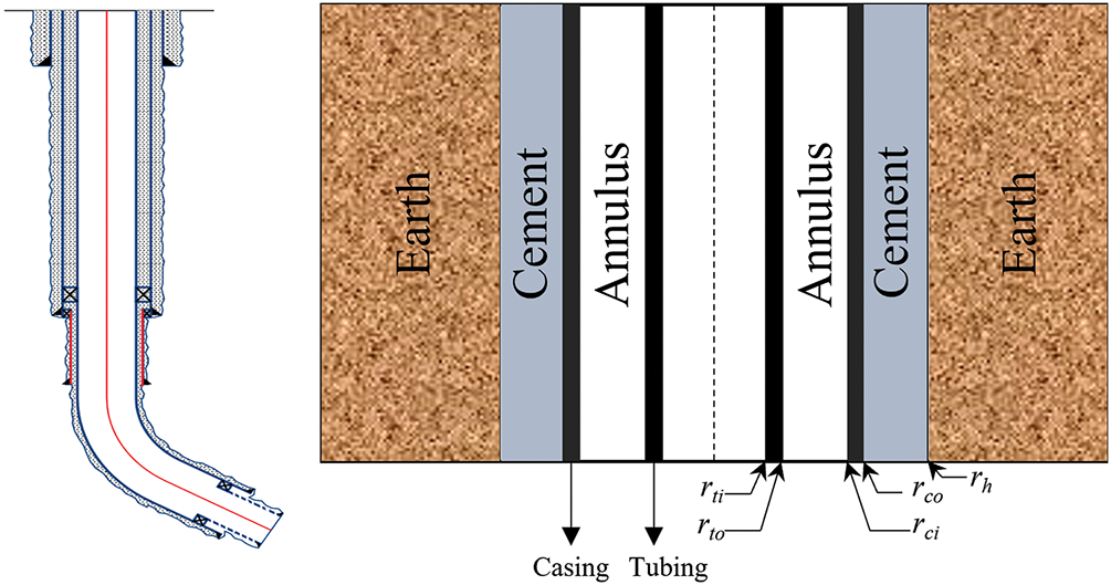
Figure 1: Schematic diagram of wellbore physical model and heat transfer profile
The one-dimensional steady-state continuity equation is established with the wellbore axis as the z-axis:
In addition, the fluid inside the tubing also follows the momentum equation:
Combining with Eqs. (1) and (2), the pressure drop equation for carbon dioxide flow in the tubing can be obtained as follows [35]:
The friction coefficient is responsible for handling the loss of fluid kinetic energy [36]. It can be calculated by the explicit formula proposed by Chen [37], which applies to any Reynolds number Re and roughness Δ:
According to the statistical data in the literature [38], the roughness range of the new oil pipe is approximately 0.0127 to 0.01524 mm. This article took 0.0152 mm.
According to Fig. 2, for one-dimensional steady-state heat transfer inside the wellbore, there is the following energy conservation equation [39]:
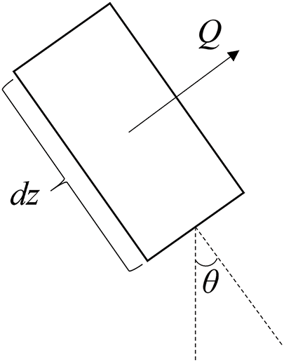
Figure 2: Schematic diagram of tubing unit section
The heat transfer Q between the tubing and the formation can be characterized by the following equation [40]:
Consider the definition of specific enthalpy (Eq. (8)) and the specific enthalpy gradient equation (Eq. (9)):
According to Eqs. (1) and (6)–(9), combined with pressure drop Formula (3), the heat transfer equation for carbon dioxide in the tubing can be derived:
The total heat transfer coefficient U depends on the heat transfer capacity of the fluid inside the tubing [41] and the surrounding medium. Willhite pointed out that the overall heat transfer coefficient is the sum of the fluid inside tubing, tubing wall, annulus fluid, casing wall, cement sheath, and formation thermal resistance. In the radius coordinate system, except for the formation and convective heat transfer areas, other thermal resistances can be obtained by integrating Fourier’s law of heat conduction (Eq. (11)).
According to the reference [42,43], the thermal resistance of convective regions is contributed by their respective heat transfer coefficients. The thermal resistance in the formation is determined using the procedure proposed by Ramey [23]. Finally, the expression for the total heat transfer coefficient U is as follows:
The forced convection heat transfer coefficient ht of tubing fluid can be calculated according to the following equation [44]:
The natural convection heat transfer coefficient ha in the annulus is calculated according to the parallel plate model proposed by Dropkin and Somerscales [45]:
f(t) represents the transient heat loss function, which is time-dependent. We use the empirical formula proposed by Chiu and Thakur, which is effective at any time, to calculate it [46]:
2.4 The Calculation of CO2 Thermodynamic and Transport Properties
In contrast to methane and water, the thermophysical properties of CO2 are sensitive to temperature and pressure [47]. It is imperative that precise models are adopted in order to adequately describe these properties. The S-W Helmholtz free energy equation was utilized to calculate the thermodynamic properties of CO2, as demonstrated in the subsequent equation:
According to the above equation, the density, heat capacity and Joule-Thomson coefficient can be obtained [32]:
For the transport properties of CO2 such as viscosity and thermal conductivity, the model proposed by Vesovic and Fenghour was used to calculate them.
Eq. (22) indicates the three independent contributions of transport properties, and the specific calculation method can be found in the literature [31,33].
As explained in the previous section, solving for the temperature and pressure distribution after CO2 injection into the wellbore requires consideration of the coupling between the pressure and temperature fields and the physical properties of the CO2. To achieve this, we employed iterative methods. The specific calculation steps were as follows: First, the temperatures of the fluid inside the tubing, the inner wall of the tubing, the outer wall of the tubing, and the inner wall of the casing were assumed. Then, the pressure field could be converged. Finally, the convergence of the CO2 fluid temperature inside the tubing was determined by calculating the total heat transfer coefficient. If it did not converge, the temperature was assumed again to continue the calculation. If it converged, the calculation of the next depth began. From this, the temperature and pressure distribution within the entire tubing can be obtained. For the convenience of understanding, the solving algorithm of the model is shown in Fig. 3.
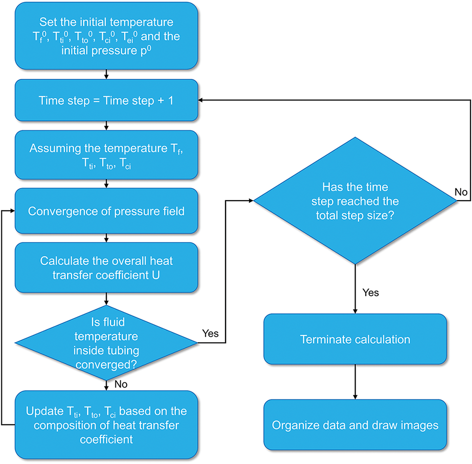
Figure 3: Model solving algorithm
As only vertical wells have actual measured temperature and pressure data in the literature, the model was modified to reflect this. The temperature and pressure distribution after 13 h of carbon dioxide injection into the tubing was iteratively solved based on on-site injection data [48]. The results are shown in Fig. 4. Under the simulation of on-site injection, it can be seen that the temperature and pressure of CO2 in the tubing showed a continuous increase along the wellbore. However, the changes in the time domain were not significant. The comparison between the measured temperature and pressure data and the calculated data is shown in Fig. 5. As the well depth increased under the influence of gravity, the pressure of CO2 in the tubing increased linearly. The measured bottom-hole pressure is 52.02 MPa and the calculated bottom-hole pressure is 52.54 MPa. The relative error is 1%. Compared to the depth of 500~3100 m, the decrease in CO2 temperature at the depth of 0~500 m was greater. This was because as the injection time increased, the heat transfer effect between the CO2 fluid in the shallow well section and the formation was stronger. The measured bottomhole temperature is 374.15 K, and the calculated bottomhole temperature is 373.15 K, with a relative error of −0.27% (if converted to °C, the error is −1%). In summary, the calculated bottom-hole temperature and pressure values were in good agreement with the measured data. This proves the model is correct and provides effective guidance for the subsequent analysis of influencing factors.
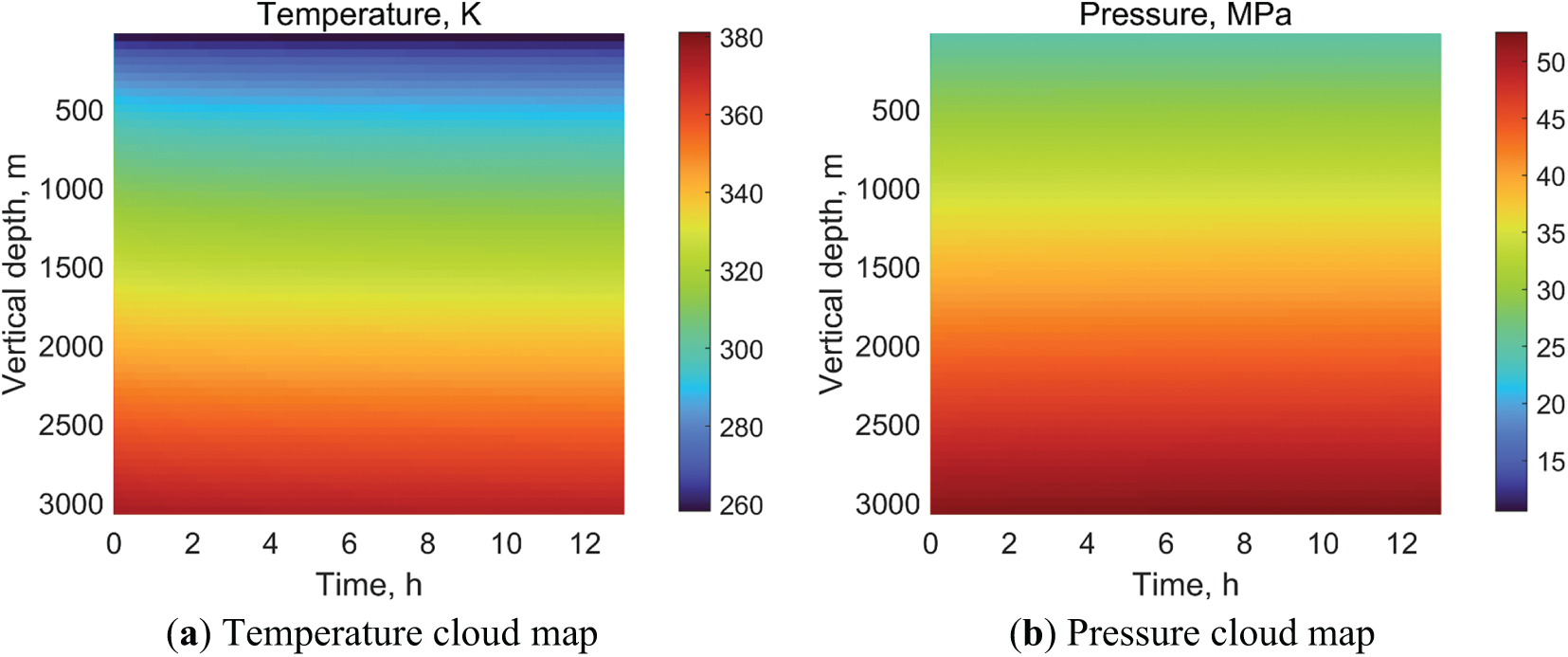
Figure 4: Temperature and pressure distribution after CO2 injection into the tubing
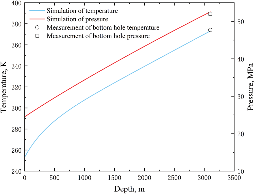
Figure 5: Comparison between measured data and calculated values
3.2 Analysis of Influencing Factors
The temperature and pressure at the bottom of the well, as the initial boundary condition of the reservoir, play a crucial role in subsequent reservoir simulation. In order to study the mechanism of changes in bottom-hole temperature and pressure, we simulated the bottom-hole temperature and pressure under different CO2 injection parameters based on the data in Table 1.
3.2.1 Different Injection Temperatures
Fig. 6 shows how bottom-hole CO2 temperature and pressure vary over time at different injection temperatures at the wellhead. As can be seen, the bottom-hole pressure increased very quickly due to gravity and then stabilized. However, there were different variations in bottom-hole pressure under different injection temperatures. An increase in injection temperature resulted in a corresponding decrease in the increase of bottom-hole pressure over a shorter time. This was because an elevated injection temperature resulted in a diminished density of CO2 within the tubing, thereby weakening the promoting effect of gravity on bottom-hole pressure. As time elapsed, the bottom-hole pressure underwent a gradual stabilization, ultimately manifesting the characteristic that an increase in injection temperature was concomitant with a decrease in bottom-hole pressure. Furthermore, an increase in injection temperature increased the CO2 temperature at the bottom of the well. Within the injection temperature range under discussion, the CO2 temperature at the bottom of the well was greater than 330 K. This meant that under normal surface injection temperature conditions, the CO2 injected for a long time at the bottom hole existed in a supercritical state (The critical pressure and temperature of CO2 are 7.38 MPa and 304.25 K).
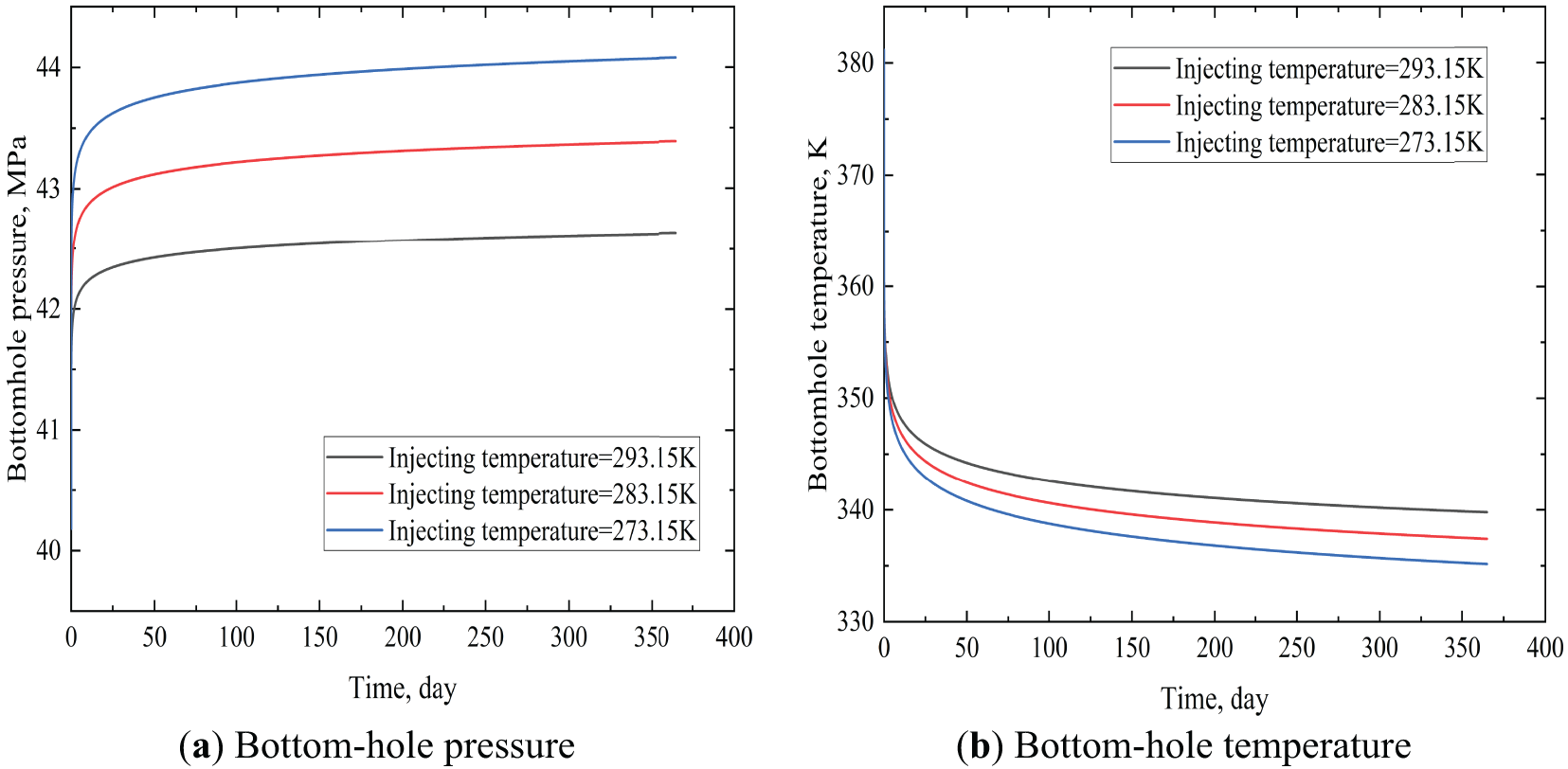
Figure 6: Bottom hole temperature and pressure at different injecting temperatures
Under different injecting temperatures, CO2 only existed in liquid and supercritical states since the CO2 pressure inside the tubing was above the critical pressure. Elevated injection temperatures reduced CO2’s thermal transfer efficiency in the tubing, yielding shallower critical-phase-transition depths and diminished liquid fractions (Fig. 7). The injection temperatures near room temperature intensified phase shifts in the tubing, substantially reducing liquid CO2 fractions while elevating supercritical CO2 (ScCO2) proportions.
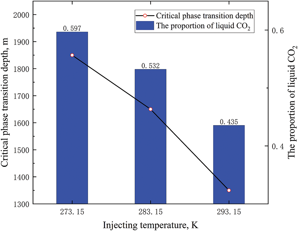
Figure 7: Phase distribution of CO2 in tubing at different injecting temperatures
3.2.2 Different Injection Pressures
As shown in Fig. 8a, the effect of different injection pressures on bottom-hole pressure was significant. At pressures ranging from 15 to 20 MPa, the bottom-hole pressure demonstrated an initial increase, subsequently reaching a state of equilibrium. However, when the injection pressure was set at 10 MPa, the bottom-hole pressure underwent an initial decrease, followed by an increase, and ultimately reached a state of stability. The underlying cause of the aforementioned phenomenon can be attributed to the fact that when the injection pressure was inadequate, the impact of tubing friction on pressure consumption was amplified, consequently leading to a diminished bottom-hole pressure at the commencement of injection in comparison to the initial state. It was observed that as the injection time was increased, the bottom-hole pressure gradually increased to a stable value. Compared to this, bottom-hole temperature decreases with injection pressure elevation (as shown in Fig. 8b). This was due to the higher heat absorption capacity of high-density carbon dioxide caused by high pressure, which led to a decrease in temperature. Nevertheless, in comparison to the alteration in bottom-hole pressure, the modification in bottom-hole temperature was negligible.
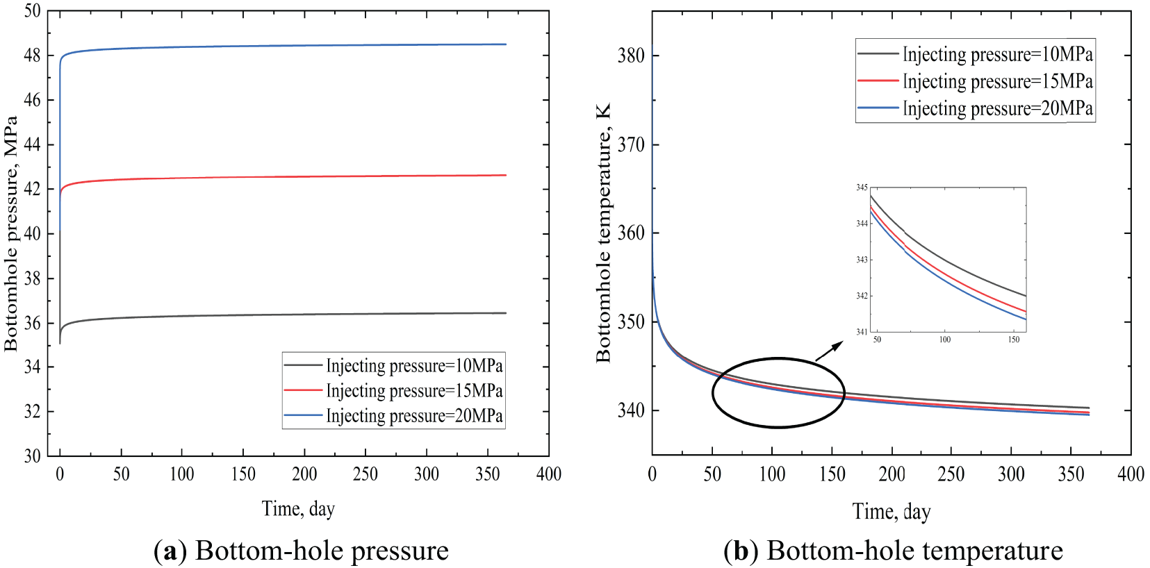
Figure 8: Bottom hole temperature and pressure at different injecting pressures
Under different injecting pressures, the influence of different injection pressures on the phase distribution of CO2 inside the tubing was relatively small (as shown in Fig. 9). The injection pressure increased by 5 MPa, and the proportion of liquid CO2 in the tubing increased by less than 5%. The well depth considered in the calculation example was 3100 m. If it was for a deeper well, the impact of injection pressure on the CO2 phase of the tubing would be smaller.
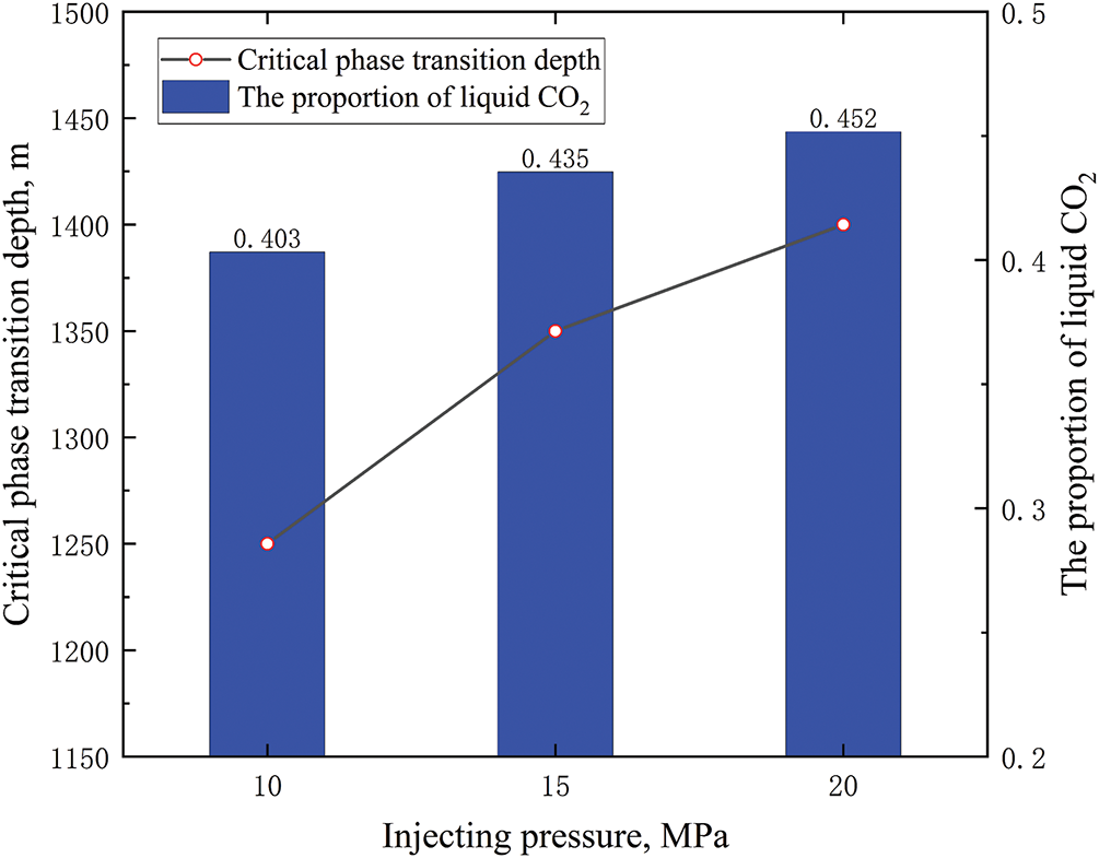
Figure 9: Phase distribution of CO2 in tubing at different injecting pressures
3.2.3 Different Injection Velocities
As shown in Fig. 10, there was a significant difference in bottom-hole temperature and pressure under different injection rates. Higher CO2 injection rates increased its accumulation density at the well bottom, thereby elevating bottom-hole pressure. Higher injection rates enhanced heat extraction capacity, accelerating the temperature decline of CO2 at the well bottom. Notably, identical increments in injection rate yielded distinct response characteristics in bottom-hole temperature vs. pressure. It was evident that if a line perpendicular to the time axis was imagined, intersecting with curves at varying injection rates at three points, it can be deduced that these three points were not equidistant. This was the result of the nonlinear term in Eqs. (3) and (10).
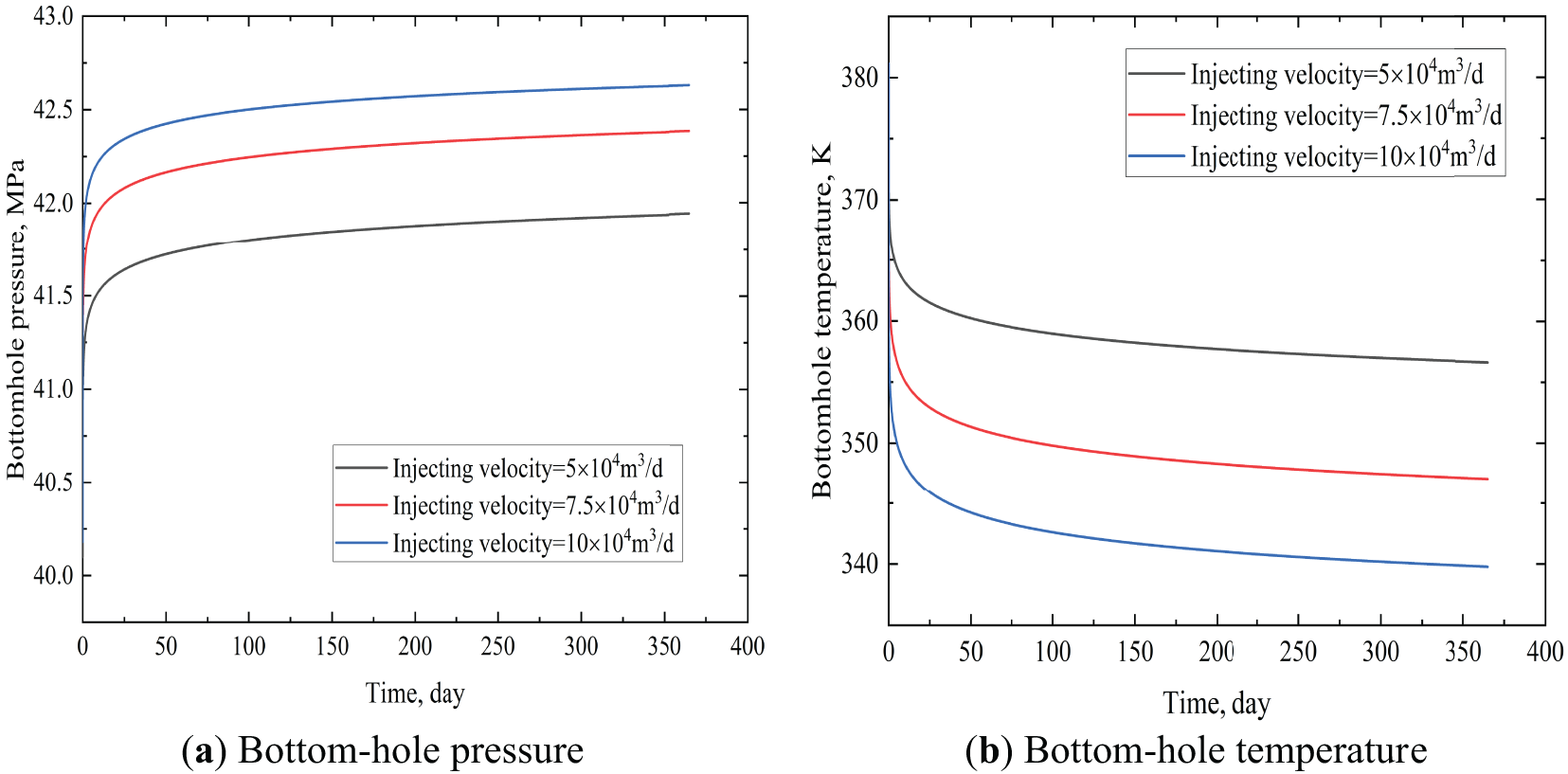
Figure 10: Bottom hole temperature and pressure at different injecting velocities
As the injection rate was increased, the critical phase transition depth of CO2 within the tubing, as well as the proportion of liquid CO2, also increased (see Fig. 11). The linear increase in the critical phase transition depth of CO2 indicated a good correspondence between the injection rate and the phase distribution of CO2 in the tubing. Consequently, in the context of actual injection processes, it is imperative to meticulously monitor the phase changes of CO2 in the tubing, triggered by fluctuations in the wellhead injection rate.
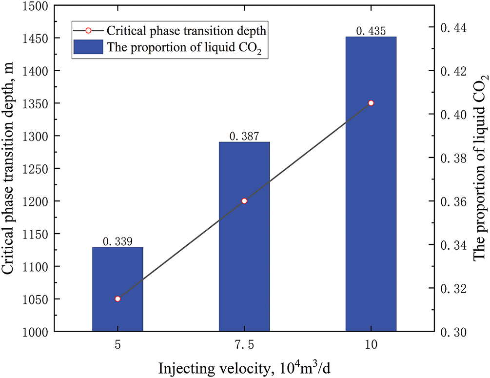
Figure 11: Phase distribution of CO2 in tubing at different injecting velocities
1. A model was developed to predict the distribution of temperature and pressure in the wellbore over time in the context of long-term CO2 injection. This model was developed using established equations, namely the steady-state heat transfer equation, the momentum equation, and the continuity equation. The solution was found by employing advanced and accurate transient heat transfer functions.
2. The injection pressure exerts a substantial influence on the bottom-hole pressure; however, its effect on the bottom-hole temperature can be disregarded. The presence of nonlinear terms in the heat transfer mechanism, relating to the injection rate, gives rise to a nonlinear response between the bottom-hole temperature and injection rate.
3. It is evident that the low injection temperature, the high injection pressure, and the injection rate can lead to an increase in the critical phase transition depth of CO2 in the tubing and an increase in the proportion of liquid CO2. However, the impact of injection pressure is minimal, with the greatest impact being exerted by injection rate, followed by injection temperature. A positive linear relationship has been observed between injection rate and critical phase transition depth.
Acknowledgement: The authors acknowledge the National Natural Science Foundation of China for providing support.
Funding Statement: This study was supported by the National Natural Science Foundation of China (Nos. 52304046, 52204051, 52174033 and U23B20156).
Author Contributions: The authors confirm contribution to the paper as follows: study conception and design: Yu Sang, Anqi Du, Yazhou Guo; data collection: Le Shen; analysis and interpretation of results: Changqing Ye, Jianhua Xiang, Yi Chen; draft manuscript preparation: Anqi Du, Le Shen. All authors reviewed the results and approved the final version of the manuscript.
Availability of Data and Materials: The datasets generated and/or analyzed during the current study are available from the corresponding author on reasonable request.
Ethics Approval: Not applicable.
Conflicts of Interest: The authors declare no conflicts of interest to report regarding the present study.
Nomenclature
| A | Cross-sectional area of the unit segment, m2 |
| Ac | Thermal conductivity area, m2 |
| cp | Isobaric specific heat capacity of fluids, J/(kg·K) |
| d | Inner diameter of tubing, m |
| E | Internal energy of fluid per unit mass, J/kg |
| f | Friction coefficient, dimensionless |
| f(t) | Transient heat loss function, dimensionless |
| g | Gravitational acceleration, 9.8m/s2 |
| Gr | Grayshev number, dimensionless |
| h | Specific enthalpy, J/kg |
| ht | Forced convection heat transfer coefficient of tubing, W/(m2·K) |
| ha | Natural convection heat transfer coefficient in the annulus, W/(m2·K) |
| k | Heat conduction coefficient, W/(m·K) |
| L | Tubing characteristic length, m |
| p | Fluid pressure, Pa |
| Pr | Prandtl number, dimensionless |
| Q | Heat transfer between tubing fluid and formation, J/s |
| Qc | Heat exchange through heat conduction, J/s |
| rh | Wellbore radius, m |
| rci | Inside radius of casing, m |
| rco | Outside radius of casing, m |
| rti | Inside radius of tubing, m |
| rto | Outside radius of tubing, m |
| R | Specific gas constant, 0.1889kJ/(kg·K) |
| Re | Reynolds number, dimensionless |
| t | Injection time, s |
| Tc | Critical temperature, K |
| Tci | Casing inside surface temperature, K |
| Te | Earth temperature, K |
| Tf | Tubing fluid temperature, K |
| Tti | Tubing inside surface temperature, K |
| Tto | Tubing outside surface temperature, K |
| U | Overall heat transfer coefficient, W/(m2·K) |
| Fluid velocity in tubing, m/s | |
| X | Transport property of CO2 |
| X0 | Contribution to the transport property in the zero-density limit |
| ΔX | Critical enhancement |
| ΔcX | Contribution of all other effects |
| z | Depth from the wellhead,m |
| Joule-Thomson coefficient, K/Pa | |
| Thermal expansion coefficient of annular fluid, 1/K | |
| Reduced density, | |
| Δ | Tubing roughness, mm |
| Helmholtz free energy, dimensionless | |
| Ideal gas part of Helmholtz free energy, dimensionless | |
| Residual fluid part of Helmholtz free energy, dimensionless | |
| Partial derivative of | |
| Well inclination angle, degree | |
| Thermal conductivity of tubing fluid, W/(m·K) | |
| Thermal conductivity of annular fluid, W/(m·K) | |
| Thermal conductivity of casing, W/(m·K) | |
| Thermal conductivity of cement, W/(m·K) | |
| Thermal conductivity of earth, W/(m·K) | |
| Thermal conductivity of tubing, W/(m·K) | |
| μ | Fluid viscosity, Pa·s |
| Annular fluid viscosity, Pa·s | |
| μf | Viscosity of fluids at qualitative temperature, Pa·s |
| μw | Viscosity of fluid at wall temperature, Pa·s |
| Tubing fluid density, kg/m3 | |
| Annular fluid density, kg/m3 | |
| Critical fluid density, kg/m3 | |
| Earth density, kg/m3 | |
| Reduced temperature, |
References
1. Feng W. Recovery enhancement at the later stage of supercritical condensate gas reservoir development via CO2 injection: a case study on Lian 4 fault block in the Fushan sag, Beibuwan Basin. Nat Gas Ind B. 2016;3(5):460–6. doi:10.1016/j.ngib.2017.02.007. [Google Scholar] [CrossRef]
2. Shi YQ, Jia Y, Pan WY, Huang L, Yan J, Zheng RC. Potential evaluation on CO2-EGR in tight and low-permeability reservoirs. Nat Gas Ind B. 2017;4(4):311–8. doi:10.1016/j.ngib.2017.08.013. [Google Scholar] [CrossRef]
3. Zhang L, Cao C, Wen S, Zhao Y, Peng X, Wu J. Thoughts on the development of CO2-EGR under the background of carbon peak and carbon neutrality. Nat Gas Ind B. 2023;10(4):383–92. doi:10.1016/j.ngib.2023.07.007. [Google Scholar] [CrossRef]
4. Heidarabad R, Shin K. Carbon capture and storage in depleted oil and gas reservoirs: the viewpoint of wellbore injectivity. Energies. 2024;17(5):1201. doi:10.3390/en17051201. [Google Scholar] [CrossRef]
5. Jones C, Spearing M, Marrion M, Maulana A, Silitonga F. A laboratory investigation of enhanced gas recovery by CO2 injection. Petro S Journ. 2025;66(1):54–66. doi:10.30632/pjv66n1-2025a4. [Google Scholar] [CrossRef]
6. Asif M, Junussov M, Longinos S, Hazlett R, Satibekova S. CO2 storage capacity of coal seams: a screening and geological review of Carboniferous coal formations of Kazakhstan. Int J Coal Sci Technol. 2025;12(1):18. doi:10.1007/s40789-025-00750-z. [Google Scholar] [CrossRef]
7. de Oliveira SB, Rocha HV, Rodrigues CFA, Lemos de Sousa MJ, Tassinari CCG. Defining CO2 geological storage capacity in unmineable coal seams through adsorption data in 3D: case study of the chico lomã deposit, southern Brazil. Sustainability. 2025;17(7):2856. doi:10.3390/su17072856. [Google Scholar] [CrossRef]
8. Izadpanahi A, Ranazzi P, Abraham-A RM, Gaeta Tassinari CC, Sampaio MA. Optimizing CO2 trapping in saline aquifers under geological uncertainty: a case study of the Rio Bonito Formation, Brazil. Gas Sci Eng. 2025;138:205593. doi:10.1016/j.jgsce.2025.205593. [Google Scholar] [CrossRef]
9. Abdul Aziz P, Marhaendrajana T, Nurhandoko BEB, Siagian UWR. Time-dependent CO2-brine-rock interaction effect on sand onset prediction: a case study of dolomite-rich sandstone in air benakat formation, South Sumatra, Indonesia. ACS Omega. 2025;10(15):14787–804. doi:10.1021/acsomega.4c09499. [Google Scholar] [PubMed] [CrossRef]
10. Huang W, Li Y, Chen P. China’s CO2 pipeline development strategy under carbon neutrality. Nat Gas Ind B. 2023;10(5):502–10. doi:10.1016/j.ngib.2023.09.008. [Google Scholar] [CrossRef]
11. Boruah A. CO2 fracturing as an alternative of hydraulic fracturing for shale gas production. In: CO2 geosequestration: capturing carbon for a sustainable future: carbon dioxide storage in geological media. Cham, Switzerland: Springer Nature; 2025. p. 59–72. doi: 10.1007/978-3-031-81021-3_4. [Google Scholar] [CrossRef]
12. Petrenko T. Study of physicochemical and geochemical aspects of enhanced oil recovery and CO2 storage in oil reservoirs. Technol Audit Prod Reserves. 2025;2(1(82)):24–9. doi:10.15587/2706-5448.2025.325343. [Google Scholar] [CrossRef]
13. Awolayo AN, Norton H, de Obeso JC, Lauer R, Crawford C, Tutolo BM. Water-Alternating-Gas (WAG) injection scheme for enhancement of carbon dioxide mineralization in basaltic aquifers. Fuel. 2025;385:134127. doi:10.1016/j.fuel.2024.134127. [Google Scholar] [CrossRef]
14. Eyitayo SI, Watson MC, Ispas I, Kolawole O. Geochemical interactions of supercritical CO2-brine-rock under varying injection strategies: implications for mechanical integrity in aquifers. Rock Mech Rock Eng. 2025. doi:10.1007/s00603-025-04496-7. [Google Scholar] [CrossRef]
15. Tosha T, Terai A, Watanabe S, Teraoka T, Kabashima T. Super-critical CO2 geothermal power generation. In: Proceedings of the 50th Workshop on Geothermal Reservoir Engineering Stanford University; 2025 Feb 10–12; Stanford, CA, USA. [Google Scholar]
16. She C, Peng H, Yang J, Peng J, Han H, Yang X, et al. Experimental study on the true triaxial fracturing of tight sandstone with supercritical CO2 and slickwater. Geoenergy Sci Eng. 2023;228(5):211977. doi:10.1016/j.geoen.2023.211977. [Google Scholar] [CrossRef]
17. Li Z, Duan Y, Peng Y, Wei M, Wang R. A laboratory study of microcracks variations in shale induced by temperature change. Fuel. 2020;280:118636. doi:10.1016/j.fuel.2020.118636. [Google Scholar] [CrossRef]
18. Li Z, Luo W, Peng Y, Cheng L, Chen X, Zhao J, et al. Investigation of the impact of supercritical carbon dioxide on the micro-mechanical properties of tight sandstone using nano-indentation experiments. Geoenergy Sci Eng. 2025;247(2):213678. doi:10.1016/j.geoen.2025.213678. [Google Scholar] [CrossRef]
19. Wang L. Study on the influence of temperature on fracture propagation in ultra-deep shale formation. Eng Fract Mech. 2023;281(23):109118. doi:10.1016/j.engfracmech.2023.109118. [Google Scholar] [CrossRef]
20. Li Z, Du Y, Duan Y, Peng Y, Li J, Ma S, et al. Microscopic experimental study on the reaction of shale and carbon dioxide based on dual energy CT mineral recognition method. Fuel. 2024;371(3):131874. doi:10.1016/j.fuel.2024.131874. [Google Scholar] [CrossRef]
21. Chen J, Yang S, Mei Q, Chen J, Chen H, Zou C, et al. Influence of pore structure on gas flow and recovery in ultradeep carbonate gas reservoirs at multiple scales. Energy Fuels. 2021;35(5):3951–71. doi:10.1021/acs.energyfuels.0c04178. [Google Scholar] [CrossRef]
22. Simangunsong MCH. Optimizing gas recovery in dry gas field “X”: CO2 injection as an effective enhanced gas recovery method [master’s thesis]. Jawa Barat, Indonesia: Institut Teknologi Bandung; 2025. [Google Scholar]
23. Ramey HJ Jr. Wellbore heat transmission. J Petrol Technol. 1962;14(4):427–35. doi:10.2118/96-pa. [Google Scholar] [CrossRef]
24. Satter A. Heat losses during flow of steam down a wellbore. J Petrol Technol. 1965;17(7):845–51. doi:10.2118/1071-pa. [Google Scholar] [CrossRef]
25. Willhite GP. Over-all heat transfer coefficients in steam and hot water injection wells. J Petrol Technol. 1967;19(5):607–15. doi:10.2118/1449-pa. [Google Scholar] [CrossRef]
26. Shiu KC, Beggs HD. Predicting temperatures in flowing oil wells. J Energy Resour Technol. 1980;102(1):2–11. doi:10.1115/1.3227845. [Google Scholar] [CrossRef]
27. Wu YS, Pruess K. An analytical solution for wellbore heat transmission in layered formations. SPE Reserv Eng. 1990;5(4):531–8. doi:10.2118/17497-pa. [Google Scholar] [CrossRef]
28. Ali SMF. A comprehensive wellbore steam/water flow model for steam injection and geothermal applications. Soc Pet Eng J. 1981;21(5):527–34. doi:10.2118/7966-pa. [Google Scholar] [PubMed] [CrossRef]
29. Wu H, Li X, He Y. A new coupled explicit finite difference model for wellbore flow and heat transfer in CO2 geological storage. Energy Proc. 2017;114(2):3597–606. doi:10.1016/j.egypro.2017.03.1491. [Google Scholar] [CrossRef]
30. Chung FTH, Li MH, Lee LL, Starling KE. An accurate equation of state for carbon dioxide. J Chem Eng Jpn. 1985;18(6):490–6. [Google Scholar]
31. Vesovic V, Wakeham WA, Olchowy GA, Sengers JV, Watson JTR, Millat J. The transport properties of carbon dioxide. J Phys Chem Ref Data. 1990;19(3):763–808. doi:10.1063/1.555875. [Google Scholar] [CrossRef]
32. Span R, Wagner W. A new equation of state for carbon dioxide covering the fluid region from the triple-point temperature to 1100 K at pressures up to 800 MPa. J Phys Chem Ref Data. 1996;25(6):1509–96. doi:10.1063/1.555991. [Google Scholar] [CrossRef]
33. Fenghour A, Wakeham WA, Vesovic V. The viscosity of carbon dioxide. J Phys Chem Ref Data. 1998;27(1):31–44. doi:10.1063/1.556013. [Google Scholar] [CrossRef]
34. Boopalan V, Rajesh KP, Arumugam SK. Numerical investigation of thermohydraulic characteristics in supercritical CO2 natural circulation loop with spatially varying temperature. Heat Transf Eng. 2025;46(9–10):822–38. doi:10.1080/01457632.2024.2347176. [Google Scholar] [CrossRef]
35. Martins IO, da Silva AK, da Silva ECCM, Hasan AR, Barbosa JR. Parametric analysis of water injection in an offshore well using a semi-transient thermal-structural model. Geoenergy Sci Eng. 2023;229(9):212055. doi:10.1016/j.geoen.2023.212055. [Google Scholar] [CrossRef]
36. Paul K, Pradhan K, Mandal BK. Effect of variation of the aspect ratio of rectangular twisted tapes inserted in a circular pipe on the thermal performance. J Therm Sci Eng Appl. 2025;17(2):021007. doi:10.1115/1.4067174. [Google Scholar] [CrossRef]
37. Chen NH. An explicit equation for friction factor in pipe. Ind Eng Chem Fund. 1979;18(3):296–7. doi:10.1021/i160071a019. [Google Scholar] [CrossRef]
38. Kumar S. Gas production engineering. Houston, TX, USA: Gulf Publishing; 1987. 646 p. [Google Scholar]
39. Li X, Li G, Wang H, Tian S, Song X, Lu P, et al. A unified model for wellbore flow and heat transfer in pure CO2 injection for geological sequestration, EOR and fracturing operations. Int J Greenh Gas Control. 2017;57(4):102–15. doi:10.1016/j.ijggc.2016.11.030. [Google Scholar] [CrossRef]
40. Hasan AR, Kabir CS. Wellbore heat-transfer modeling and applications. J Petrol Sci Eng. 2012;86(6):127–36. doi:10.1016/j.petrol.2012.03.021. [Google Scholar] [CrossRef]
41. Wu B, Liu T, Zhang X, Wu B, Jeffrey RG, Bunger AP. A transient analytical model for predicting wellbore/reservoir temperature and stresses during drilling with fluid circulation. Energies. 2017;11(1):42. doi:10.3390/en11010042. [Google Scholar] [CrossRef]
42. Hashish RG, Zeidouni M. Injection profiling through temperature warmback analysis under variable injection rate and variable injection temperature. Transp Porous Medium. 2022;141(1):107–49. doi:10.1007/s11242-021-01712-0. [Google Scholar] [CrossRef]
43. Li X. Research on flow-heat transfer and rock damage during CO2 fracturing based on multiphysics coupling [dissertation]. Beijing, China: China University of Petroleum Beijing; 2018. (In Chinese). [Google Scholar]
44. Lienhard JH. A heat transfer textbook. Hoboken, NJ, USA: Prentice Hall; 1981. 516 p. [Google Scholar]
45. Dropkin D, Somerscales E. Heat transfer by natural convection in liquids confined by two parallel plates which are inclined at various angles with respect to the horizontal. J Heat Transf. 1965;87(1):77–82. doi:10.1115/1.3689057. [Google Scholar] [CrossRef]
46. Chiu K, Thakur SC. Modeling of wellbore heat losses in directional wells under changing injection conditions. In: Proceedings of the SPE Annual Technical Conference and Exhibition; 1991 Oct 6–9; Dallas, TX, USA. doi:10.2118/22870-MS. [Google Scholar] [CrossRef]
47. Kang J, Vorobiev A, Cameron JD, Morris SC, Turner MG, Sedlacko K, et al. Experimental study of the real gas effects of CO2 on the aerodynamic performance characteristics of a 1.5-stage axial compressor. J Eng Gas Turbines Power. 2025;147(8):081012. doi:10.1115/1.4067267. [Google Scholar] [CrossRef]
48. Yi LP, Li XG, Yang ZZ, Sun J. Coupled calculation model for transient temperature and pressure of carbon dioxide injection well. Int J Heat Mass Transf. 2018;121(8):680–90. doi:10.1016/j.ijheatmasstransfer.2018.01.036. [Google Scholar] [CrossRef]
Cite This Article
 Copyright © 2025 The Author(s). Published by Tech Science Press.
This work is licensed under a Creative Commons Attribution 4.0 International License , which permits unrestricted use, distribution, and reproduction in any medium, provided the original work is properly cited.
 Downloads
 Citation Tools