
 Submit a Paper
 Propose a Special lssue
 Open Access
ARTICLE

Six-Degree-of-Freedom Motion Analysis of High-Speed Craft Navigating through Variable Marine Environments
1 China Coast Guard Academy, Ningbo, 315801, China
2 Ningbo Key Laboratory of Green Shipping Technology, Faculty of Maritime Transportation, Ningbo University, Ningbo, 315211, China
* Corresponding Author: Min Kuang. Email:
(This article belongs to the Special Issue: Recent Advancements in Wave Dynamics Models for Fluids: Analytical and Numerical Approaches)
Fluid Dynamics & Materials Processing 2025, 21(9), 2201-2223. https://doi.org/10.32604/fdmp.2025.067081
Received 24 April 2025; Accepted 13 August 2025; Issue published 30 September 2025
 View Full Text
 Download PDF
Abstract
The dynamic behavior of high-speed craft navigating through variable sea states plays a pivotal role in ensuring maritime safety. However, many existing simulation approaches rely on linear or overly simplified representations of the marine environment, thereby limiting the fidelity of motion predictions. This study explores the motion characteristics of a 4.5-t high-speed vessel by conducting fully coupled numerical simulations using the STAR-CCM+ software. The analysis considers both calm and varying sea conditions, incorporating fluctuations in wave height, wavelength, and wind speed to reflect more realistic operating scenarios. Simulation results reveal that the vessel’s hydrodynamic response is highly sensitive to changes in sea state. As conditions deteriorate, the free surface becomes increasingly complex, with higher wave amplitudes and more pronounced interactions between the waves generated by the vessel and those imposed by the external environment. These effects lead to significant increases in roll, pitch, heave, and sway motions, thereby imposing greater demands on the vessel’s dynamic stability and operational safety. Furthermore, both hydrodynamic resistance and propulsive thrust exhibit notable dependence on sea state and vessel speed. Total resistance generally increases with rougher sea conditions, while thrust tends to rise with increasing forward speed. Under calm or mildly disturbed waters, a Froude number (Fr) of 0.5 appears to offer an optimal balance for initiating and controlling primary motions such as roll, pitch, heave, and sway. Conversely, in more challenging conditions—such as those represented by a Sea State 3—effective motion control is better achieved at a higher Froude number of approximately 1.0.Keywords
High-speed craft play a crucial role in various marine applications, including transportation, military operations, and sea rescue. However, their performance in complex sea conditions is significantly influenced by multiple factors, particularly the sea state. Understanding their motion characteristics under different sea conditions is essential for ensuring navigation safety and operational efficiency. Compared to displacement vessels, high-speed small boats exhibit more complex hydrodynamic behavior. Their operation is dominated by hydrodynamic and hydrostatic forces, which are closely linked to speed. Additionally, factors such as wave and viscous drag, waterjet propulsion, nonlinear motion, and instability complicate their analysis.
Current research often simplifies sea states, leading to inaccurate motion predictions. To address coupled motion, Lewandowski et al. [1] proposed an empirical formula for the combined effects of rolling, swaying, and yawing based on a simplified model. However, the linear assumptions of this model reduce its applicability under conditions involving large motions or strong nonlinear wave loads. Lewandowski’s results are valid in calm water and small-amplitude waves, but the errors are large in cases of large motions or strong nonlinearity. In predicting the hydrodynamic performance of skiffs and high-speed vessels, the empirical method proposed by Savitsky [2] provides a practical tool for preliminary design by estimating drag, trim angle, and lift. However, it is limited in accounting for nonlinear fluid effects, such as those involving large slant angles or instability at high speeds. Using wave-current interaction theory, Griffin [3] studied turbulent wake-induced surface currents modifying ship Kelvin wakes. Results show currents narrow wake angles, shift wave directions, and shorten wavelengths, qualitatively matching SAR observations. Limitations involve oversimplified uniform currents, excluded transverse/nonlinear effects, inability to explain very narrow wakes with realistic currents, and ignored ambient factors. Mariya et al. [4] experimentally identifies linear inertial wave regimes (attractors, global oscillations) generating stable vortices, akin to high-speed craft motion in mild sea states. Nonlinear triadic resonance instabilities and vortex drift mirror severe wave-craft interactions; however, unresolved 3D boundary effects and limited theoretical modeling restrict its applicability to complex hydrodynamic systems. Blount et al. [5] pointed out that the dynamic instability mechanisms of high-speed craft differ significantly from those of traditional ships. However, further research is needed to deepen understanding of their nonlinear behavior at high speeds. Li et al. [6] investigated cavitating flows around a hydrofoil, highlighting the impact of flow conditions. This study aims to overcome limitations by comprehensively analyzing high-speed craft motion under variable sea states to ensure navigation safety.
Yasukawa et al. [7] investigated the effects of boat speed, attitude, and stern attachments on maneuverability using both experiments and simulations. However, calm water test conditions are difficult to replicate in practice, as they fail to account for wave effects and multi-degree-of-freedom coupling. Belga et al. [8] demonstrated that the prediction accuracy of traditional potential flow theory is insufficient for modern high-speed ship types (e.g., trimarans) or under extreme sea conditions. Shi et al. [9] employed TEBEM with ship-wave coupling to study ship motions in waves, showing improved accuracy; limitations involve high computational cost and exclusion of strong nonlinearities/viscous effects. Takami et al. [10] employed active learning Kriging+Markov Chain Monte Carlo (AK-MCMC) with Karhunen–Loève (KL) expansion of ocean wave to study extreme nonlinear ship responses, showing superior efficiency and accuracy in failure probability and Mean-out-crossing rate estimations compared to FORM; limitations involve computational burden for high-dimensional cases and potential inaccuracies for extreme events with long memory time. Wu et al. [11] used a spectral-coupled BEM with overset mesh and attention mechanisms to efficiently simulate nonlinear ship waves (Wigley/S60 hulls), validating wave run-up and resistance accuracy; limitations include ignored viscous effects and inability to capture breaking waves.
Tavakoli et al. [12] validated the 2D+T method for predicting turning radius and longitudinal and lateral oscillations. However, the method’s sensitivity to errors in forward motion requires further refinement. Park et al. [13] used high-fidelity CFD to simulate the six-degree-of-freedom (6-DOF) motion of a high-speed vessel. The results were consistent with safety standards, though the influence of wave interference was not fully examined. Cao [14] and Shen et al. [15] employed Fluent and dynamic mesh techniques to develop numerical optimization strategies for unsteady flow around moving bodies with multiple degrees of freedom. These strategies significantly improved the accuracy of lift and drag force calculations. Yao et al. [16] used the RANS model in OpenFOAM to evaluate the response of a ship to yawing motion. However, discrepancies in added drag forces revealed the need to enhance the flow model. In the area of coupled dynamic systems. Yu et al. [17] introduced a LS-DYNA coupled model that, for the first time, enabled simultaneous analysis of ship collisions/grounding and six-degree-of-freedom motion.
From the above studies, it is evident that the prediction accuracy of empirical methods decreases when applied to high-speed craft or extreme sea states. Moreover, many studies consider only linear conditions or simplified sea states, which limits their ability to fully and accurately reflect the real motion behavior of high-speed craft. The innovation of this study lies in overcoming the limitations of using a single sea state parameter or linear assumptions in traditional research. A variable sea state model is constructed with multi-parameter coupling of wave height, wave length, wind speed, and vessel speed, which systematically reveals the nonlinear response mechanisms of 6-DOF motion in high-speed craft under complex wave environments. Therefore, studying the six-degree-of-freedom motion characteristics of high-speed craft during straight-line sailing under different sea conditions has both practical significance and theoretical value. The research outcomes contribute to the safe and stable navigation of high-speed vessels. In this study, a validated numerical simulation approach is used to analyze a 4.5-t high-speed craft under variable sea conditions. The objective is to recommend optimal navigation parameter settings for different sea states in line with the craft’s safety requirements.
2 High-Speed Craft and Methodology
The 4.5-t manned high-speed craft, shown in Fig. 1, is a wave-piercing, deep V-type monohull with a single bottom and single deck. Both the main hull and the superstructure deckhouse are constructed from composite materials. Its design speed under full load in open water is not less than 30 knots, assuming wind speeds do not exceed Beaufort scale grade 3 and water depth is at least 10 m. The vessel has an endurance of 8 h at a cruising speed of 18 knots under sea state conditions of Grades 1–2. The main design parameters are listed in Table 1. The hull was modeled using Maxsurf software, and the hull line drawing is shown in Fig. 2.

Figure 1: Manned high-speed workboat.

Figure 2: Cross-section of workboat hull.
Table 1: Main design parameters of manned high-speed workboats.
| Item | Value |
|---|---|
| Overall length (LOA) | 9.00 M |
| Waterline length (LWL) | 7.78 M |
| Overall beam (BOA) | 3.20 M |
| Beam (B) | 2.98 M |
| Depth (D) | 1.50 M |
| Height (H) | 3.50 M |
| Design draft (T) | 0.68 M |
| Displacement (D) | 4.5 t |
The free navigation of the high-speed craft under different sea conditions and speeds is simulated in still water and in sea states 1 to 3. The operational conditions for each simulation case are shown in Table 2. A total of 16 simulation cases are considered, combining various sea conditions and speeds. For each sea state—still water and Grades 1 through 3—four Fr are used to simulate different speeds.
Table 2: Simulation case parameters.
| Case Order | Fr | Speed (m/s) | Wave Height (m) | Wave Length (m) | Wind Speed (m/s) | Sea State |
|---|---|---|---|---|---|---|
| 1 | 0.5 | 4.70 | 0 | 0 | 0 | Calm water |
| 2 | 1.0 | 9.39 | 0 | 0 | 0 | |
| 3 | 1.5 | 14.09 | 0 | 0 | 0 | |
| 4 | 2.0 | 18.78 | 0 | 0 | 0 | |
| 5 | 0.5 | 4.70 | 0.055 | 1.8 | 0.3 | First sea condition |
| 6 | 1.0 | 9.39 | 0.055 | 1.8 | 0.3 | |
| 7 | 1.5 | 14.09 | 0.055 | 1.8 | 0.3 | |
| 8 | 2.0 | 18.78 | 0.055 | 1.8 | 0.3 | |
| 9 | 0.5 | 4.70 | 0.3 | 4.5 | 2.5 | Second sea condition |
| 10 | 1.0 | 9.39 | 0.3 | 4.5 | 2.5 | |
| 11 | 1.5 | 14.09 | 0.3 | 4.5 | 2.5 | |
| 12 | 2.0 | 18.78 | 0.3 | 4.5 | 2.5 | |
| 13 | 0.5 | 4.70 | 0.8 | 9.0 | 5.0 | Third sea condition |
| 14 | 1.0 | 9.39 | 0.8 | 9.0 | 5.0 | |
| 15 | 1.5 | 14.09 | 0.8 | 9.0 | 5.0 | |
| 16 | 2.0 | 18.78 | 0.8 | 9.0 | 5.0 |
In this study, the numerical calculations of hydrodynamic characteristics at different Fr are conducted using the STAR-CCM+ software platform. The Navier-Stokes (N-S) equations are used to simulate the flow field around the craft. The Reynolds-Averaged Navier-tokes (RANS) method is applied to solve the N-S equations, using the continuity and momentum equations, expressed as:
The continuity equation (mass conservation):
The standard form of RANS momentum equation:
Regarding the load issue of high-speed boats in waves, the fluid is generally regarded as an incompressible fluid. The fluid density does not change with time, that is, the density ρ of the fluid can be considered as a constant. Therefore, the first term of the continuity equation for the fluid can be zero, that is: ∂ρ/∂t = 0. Therefore, the continuity equation for fluids is simplified to:
The component forms are as follows:
Energy conservation is neglected as the flow is isothermal, consistent with typical maritime simulations. The SST k-ω model in STAR CCM+ blends k-ω (near-wall accuracy without wall functions) and k-ε (free-stream reliability) via a blending function. It handles adverse pressure gradients and flow separation better than standard k-ω (over-predicts eddy viscosity in free streams) or k-ε (relies on wall functions, poor near-wall resolution), crucial for ship hull/propeller flows. So the turbulence model used is the k-ω SST model, whose governing equations are:
For simulating the maneuvering motion of the high-speed craft under wave conditions, a VOF wave model in STAR-CCM+ is used to numerically simulate gravity waves between the water and air phases. In the VOF framework, density
Wavefront height equation:
Horizontal velocity equation for waves:
Vertical velocity equation for waves:
In the above equations,
As the wave length increases rapidly with vessel speed, the wake angle—defined between the wake and the longitudinal centerline—becomes much narrower than that of conventional boats. To account for this, the computational domain is extended longitudinally downstream of the hull, while the width-wise extension is appropriately constrained. The dimensions of the entire computational domain are shown in Fig. 3. Given the flow symmetry, only one half of the hull is modeled. The velocity inlet is located one boat length upstream of the bow, while the pressure outlet is two boat lengths downstream of the stern. The side boundaries, defined as symmetry planes, are set two boat lengths from the centerline. The top and bottom boundaries are treated as velocity inlets, located one and two boat lengths from the hull, respectively.

Figure 3: Computational domain dimensions and boundary conditions.
The background grid of the entire computational domain and the overlapping grid around the hull are both cut-cell grids. According to Zou et al. [24], the surface grid size of the hull is selected to be 0.4–0.9% of the boat length; in this study, it is set at 0.6% of the boat length. A boundary-layer grid is arranged along the hull surface. To accurately capture the free surface, particularly the bow and stern wave patterns, anisotropic mesh refinement is applied to the free surface area at the bow, stern, and throughout the computational domain. The mesh size is set to 0.8% of the boat length in the x- and y-directions, and 0.4% in the z-direction. A linear interpolation scheme is used for data exchange between the overlapping and background meshes. A representative mesh of the high-speed craft is shown in Fig. 4.
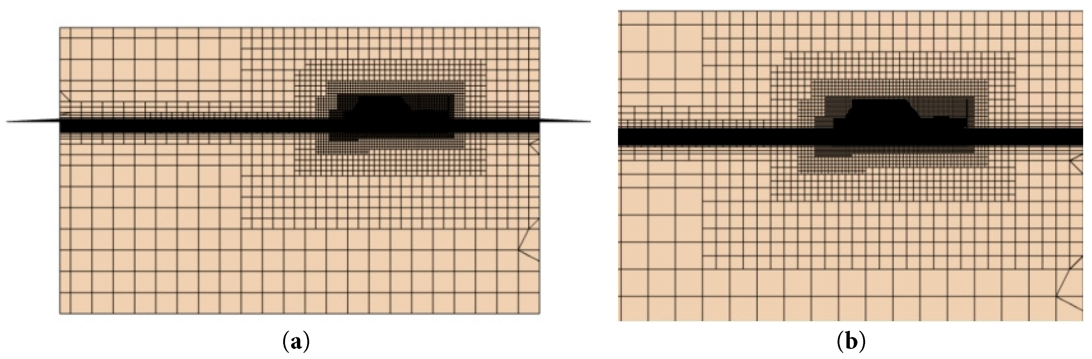
Figure 4: Calculation domain and meshing form. (a) Calculation domain; (b) Local zoomed-in meshing.
For grid-independence verification, different mesh densities are generated using a step-by-step refinement method. Grid independence is considered achieved when the relative errors between computational results from different grid densities fall below a predetermined threshold. Grid convergence is validated using the Richardson extrapolation method. A triple-mesh sequence with a refinement ratio of
Table 3: Number of grid cells in the triple-series mesh.
| Grid Density | Grid Program | Number of Grids (million) |
|---|---|---|
| Fine | Grid 1 | 3.086 |
| Medium | Grid 2 | 2.055 |
| Coarse | Grid 3 | 1.335 |
In this paper, the SIMPLE algorithm [25] is used to solve the pressure-velocity coupling problem. The momentum and turbulent variables are discretized using the second-order upwind scheme; the VOF interface reconstruction employs the HRIC (High Resolution Interface Capture) first-order scheme [26]. An implicit unsteady model [22,23] with a second-order time step is adopted; the time step is set to 0.01 s to ensure that the CFL number is less than 1.0 to guarantee stability. The meshing is performed using a hexahedral mesh with surface reconstruction, automatic surface repair, and prism layers, which has been verified in ship fluid dynamics.
Fig. 5 compares results for roll, pitch, heave, and drag for the high-speed craft under hydrostatic free-sailing conditions at Fr = 1.0. Although the computational domain assumes left-right symmetry, free navigation may induce roll due to model errors, numerical noise in simulations, and tiny perturbations in initial conditions, which disrupt the symmetric condition.
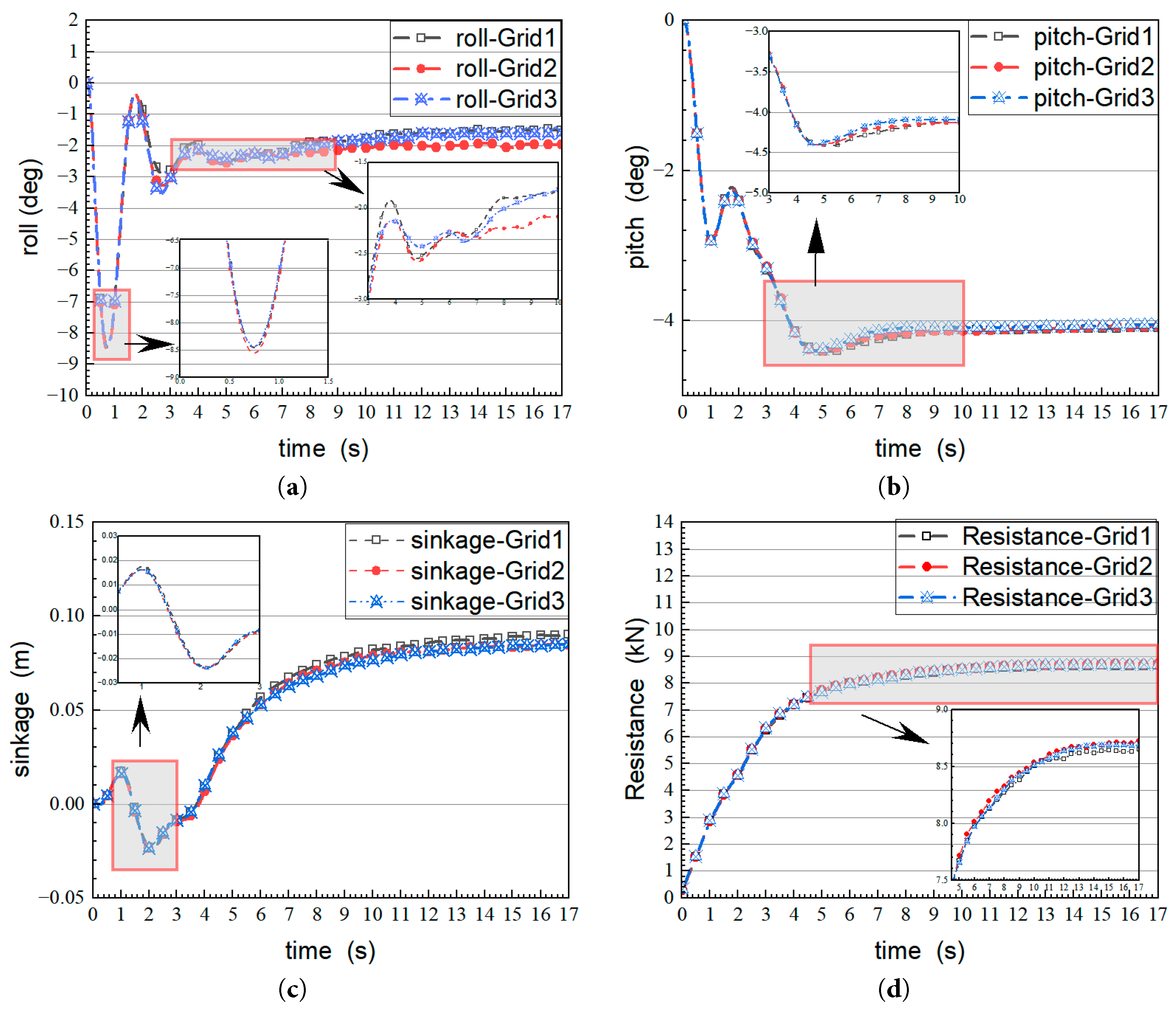
Figure 5: Grid-independence verification based on roll, pitch, sinkage, and resistance comparisons. (a) Roll; (b) Pitch; (c) Sinkage; (d) Resistance.
In Fig. 5a, the roll amplitude and phase characteristics of the 2.055 million and 3.086 million grid cases show strong agreement (error < 5%). In Fig. 5b, the pitch angle curves of the same two grids nearly overlap (maximum deviation < 0.2°). In Fig. 5c, the heave amplitudes for the 2.055 million grid (0.08–0.10 m) and 3.086 million grid (0.09–0.10 m) are similar, while the 1.335 million grid shows more fluctuation, indicating that the medium-density grid sufficiently captures the free surface behavior. The resistance comparison in Fig. 5d shows excellent agreement between the 2.055 million and 3.086 million grids, with the 1.335 million grid exhibiting an error within 5%. Although the 3.086 million-grid solution shows slightly higher accuracy than the 2.055 million-grid case, the increase in computational time is substantial, while the improvement in results is less than 2%, which does not align with the principle of efficiency in engineering simulations. Considering both computational efficiency and accuracy, the 2.055 million-grid configuration is selected for subsequent simulations.
To validate its impact on accuracy, we conducted additional simulations with three domain configurations: ① 1L upstream and 2L downstream, ② 1L upstream and 3L downstream, ③ 1L upstream and 4L downstream. In Table 4, the number of grids set for these three domain is shown. All cases extended the simulation time to 50 s to ensure steady-state convergence.
Table 4: Number of grid cells in the triple-series mesh.
| Grid Density | GRID Program | Number of Grids (million) |
|---|---|---|
| ① | Grid 2 | 2.055 |
| ② | Grid 4 | 2.875 |
| ③ | Grid 5 | 3.698 |
As shown in the supplementary data in Fig. 6, the discrepancies in key parameters (e.g., resistance, heave amplitude) among the three schemes were within 5%, confirming that the domain size has a negligible effect on results beyond 2L downstream. However, schemes ② and ③ required 24% and 32% more computational time than scheme ①, respectively, due to the increased mesh quantity and integration steps.
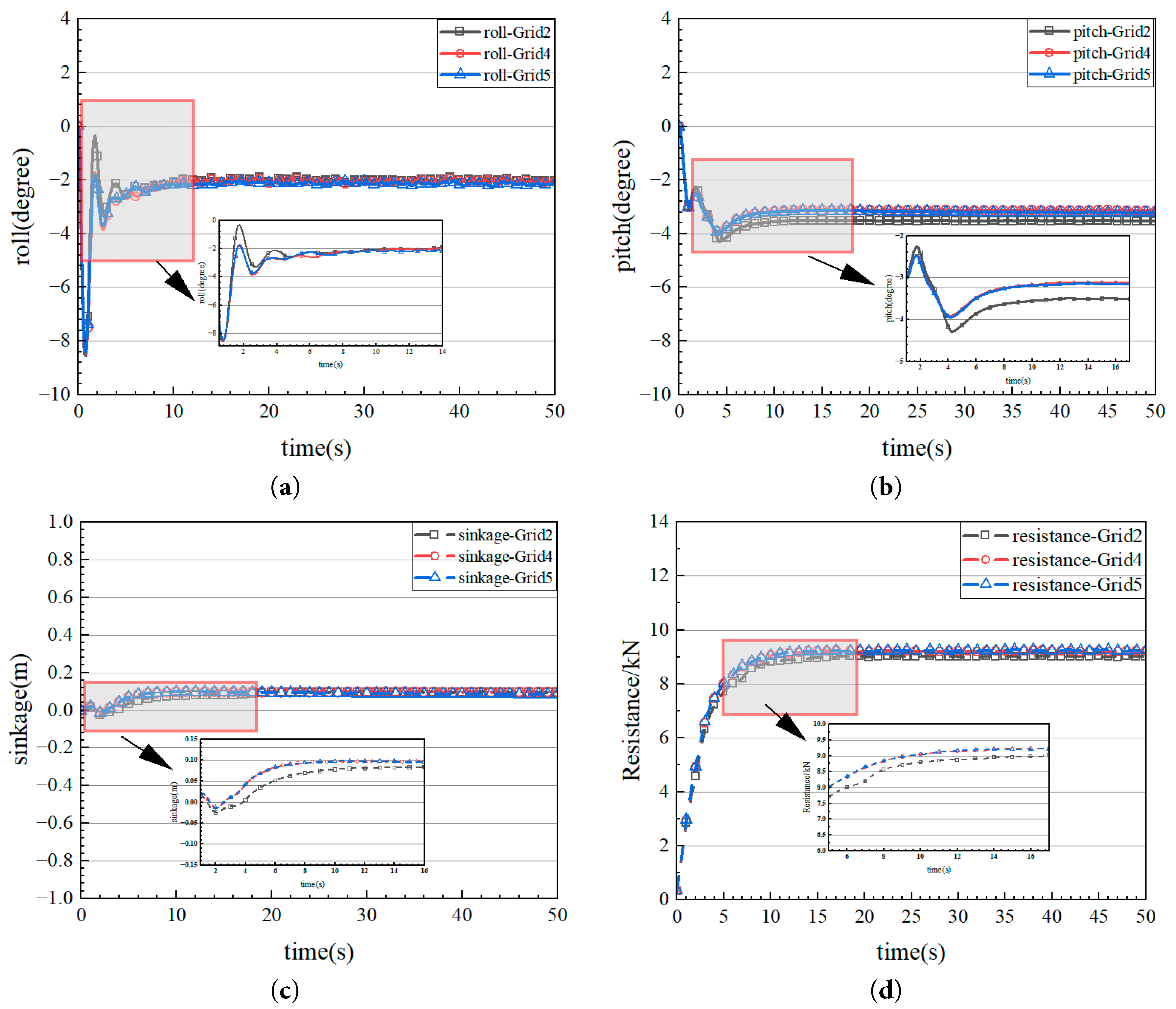
Figure 6: Grid-independence verification based on roll, pitch, sinkage and resistance comparisons. (a) roll; (b) pitch; (c) sinkage; (d) resistance.
Considering the trade-off between accuracy and efficiency, scheme ① (1L upstream, 2L downstream) was selected. This configuration not only meets the precision requirement (error < 5%) but also optimizes computational resources. The validation results have been added to Section 2.2 to clarify the domain sensitivity analysis.
As the high-speed craft studied in this paper lacks experimental data, the validity of the simulation method is verified using data from literature [27], which provides tested results for a similar high-speed C model craft from the Taunton series. The main parameters of the C model craft are provided in Table 5. Fig. 7 shows its simulation model, which incorporates the PPTC standard propeller to create a virtual disk body that acts as thrust for the modeled craft.
Table 5: Main dimensions of the Taunton-C glide boat model [27].
| Main Dimensions | Value |
|---|---|
| Overall length (LOA) | 2.0 m |
| Beam (B) | 0.46 m |
| Draft (T) | 0.09 m |
| Displacement (D) | 24.81 kg |
| Deadrise angle (β) | 22.5° |
| Longitudinal position of the center of gravity (LCG/L) | 0.33 |
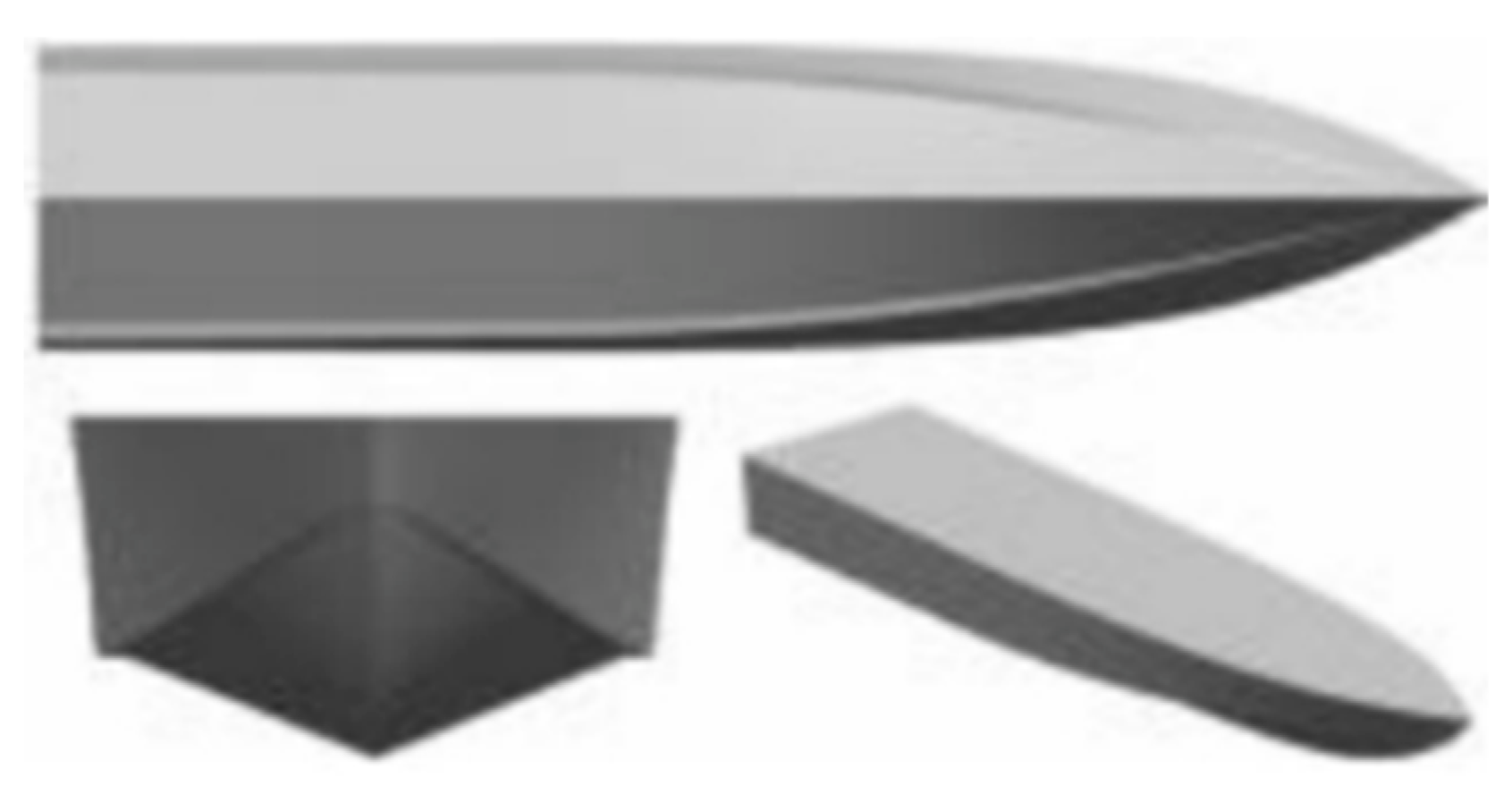
Figure 7: Schematic diagram of Taunton-C glide boat model [27].
Following the CFD testing and validation protocol recommended by the ITTC [28], simulations were performed using three different meshing schemes, listed in Table 3, under still water conditions at speeds of 4.08, 8.13, and 12.05 m/s. Validation is achieved by comparing measured values (denoted as D in Table 5) with simulated results for navigational drag. The corresponding drag curves are presented in Fig. 8. Table 6 summarizes the key data from the validation process. Here RG is the convergence rat, pG is the accuracy order, |1 − CG| is the absolute deviation of the correction coefficients (i.e., the estimation error), UG is the final uncertainty estimation, UD is the uncertainty of the difference, UV is the uncertainty of the error, |E| is the comparative error, and D refers to the experimental data from Table 7. As shown in Fig. 8, all computed drag results demonstrate monotonic convergence, except for the third scheme with a sparse grid density. At all three speeds, the calculated drag values for the remaining two meshing schemes show good agreement with the measured data. Table 6 indicates that the drag results at 4.08 and 12.05 m/s (i.e., |E| < UV) are well validated. Although the comparison error at 8.13 m/s slightly exceeds the uncertainty of the error (|E| > UV), it is still within a feasible range based on uncertainty analysis. From the standpoint of computational accuracy, the maximum drag prediction error using the dense grid scheme is 7.62%. According to the 27th ITTC conference, for CFD resistance predictions of unconventional ship types (e.g., multihulls, skiffs, or novel designs), an error margin of less than 10% compared to model tests is considered acceptable.
Table 6: Validation of navigational resistance accuracy [27].
| Speed (m/s) | RG | pG | |1 − CG| (%) | UG (%) | UD (%) | UV (%) | |E| (%) | |
|---|---|---|---|---|---|---|---|---|
| 4.08 | 0.81 | 0.60 | 0.77 | 7.02 | 17.79 | 3.20 | 18.07 | 4.61 |
| 8.13 | 0.37 | 2.88 | 0.72 | 1.03 | 2.50 | 2.70 | 3.38 | 7.62 |
| 12.05 | 0.39 | 2.71 | 0.56 | 8.08 | 17.16 | 2.40 | 17.32 | 5.51 |
Table 7: Experimental data D [27].
| Speed (m/s) | Resistance (n) |
|---|---|
| 4.08 | 36.98 |
| 8.13 | 49.79 |
| 12.05 | 82.31 |
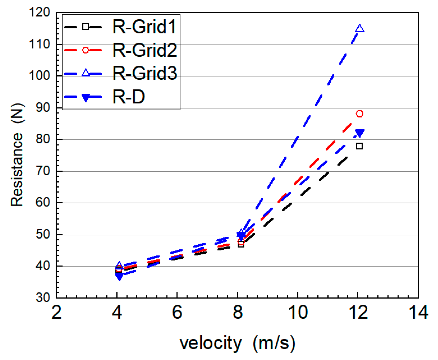
Figure 8: Comparison of calculated and measured navigational resistance for three grid schemes of the Taunton-C high-speed craft.
Under four sea conditions—calm water, Sea State I (wave height 0.055 m, wave length 1.8 m, wind speed 0.3 m/s, windward), Sea State II (wave height 0.3 m, wave length 4.5 m, wind speed 2.5 m/s, windward), and Sea State III (wave height 0.8 m, wave length 9 m, wind speed 5.0 m/s, windward)—free-running motion simulations were carried out for a high-speed craft at Fr = 0.5, 1.0, 1.5, and 2.0. The wave setup in all sea conditions is head sea.
As illustrated in Fig. 9, the temporal variations in the free-surface wave pattern of the craft at Fr = 1.5 are shown for each sea state. In calm water, the ship-generated wave exhibits a characteristic V-shaped wake with a regular and symmetrical crest line and minimal amplitude (approximately 0.05 m). The wave propagates in the sailing direction with a diffusion angle of approximately 15°, which aligns with the theoretically predicted wake angle. At this stage, the free surface is influenced solely by the vessel’s motion, with no interference from ambient waves. In Sea State I, the free surface is a result of the superposition of the ship-generated wave and the ambient wave. The ship-generated wave remains dominant, though the amplitude increases to 0.12 m and local waveform distortions appear. The wave energy remains low, and the interference is primarily linear.


Figure 9: Free-surface plots for the high-speed craft sailing freely at Fr = 1.5. (a) Still water; (b) First-class sea state; (c) Second-class sea state; (d) Third-class sea state.
In Sea State II, nonlinear interactions between the ship-generated and ambient waves intensify, increasing the wave amplitude to 0.35 m. The waveform exhibits clear peak breaking and vortex structures. The diffusion angle of the V-shaped wake narrows to 10°, indicating significantly increased wave resistance at high speed.
In Sea State III, the ambient wave becomes dominant, with the free-surface wave amplitude reaching 1.2 m. More than 60% of the waves are breaking. The ship-generated wake is fully submerged, the waveform becomes highly irregular, and significant splash flow appears at the bow, dynamically altering the wetted hull area. At this stage, strong coupling between the waves and hull induces large vertical shock loads, exacerbating kinematic instability. The 10° wake angle at Fr = 1.5 aligns with Michell’s theory regarding the narrowing of the wake at critical speeds. The observed vortex generation is consistent with Faltinsen’s nonlinear wave theory [29].
In ideal symmetric conditions (head sea waves with left-right hull symmetry), pure surge, heave, and pitch motions are theoretically expected, with roll and sway components ideally zero due to symmetry. However, the presence of small roll/sway amplitudes in our simulations can be attributed to the following factors:
The errors in CFD mainly come from model errors and numerical errors. Numerical errors can be reduced by improving the discretization accuracy. In ideal symmetric conditions (head sea waves with left-right hull symmetry), pure surge, heave, and pitch motions are theoretically expected, with roll and sway components ideally zero due to symmetry. However, the presence of small roll/sway amplitudes in our simulations can be attributed to the following factors: Numerical noise: Small discretization errors or iterative solver fluctuations in CFD can introduce asymmetric velocity/pressure fields, even in symmetric domains. Initial perturbations: Minor deviations in initial conditions can amplify through nonlinear fluid-structure interactions. Hull imperfections: Subtle geometric asymmetries (e.g., manufacturing tolerances, asymmetric mesh refinement) not captured in the idealized symmetric model may induce asymmetric hydrodynamic forces.
Fig. 10 presents the roll response characteristics of the high-speed craft under the four sea states and varying Fr. The results show a progressive increase in roll amplitude with both sea state severity and vessel speed. In calm water (Sea State 0), the craft exhibits minimal rolling (amplitude < 9.06°) and stable oscillatory behavior. As sea state severity increases from I to III, the amplitude grows approximately quadratically with wave height [30], accompanied by increasingly nonlinear response features.
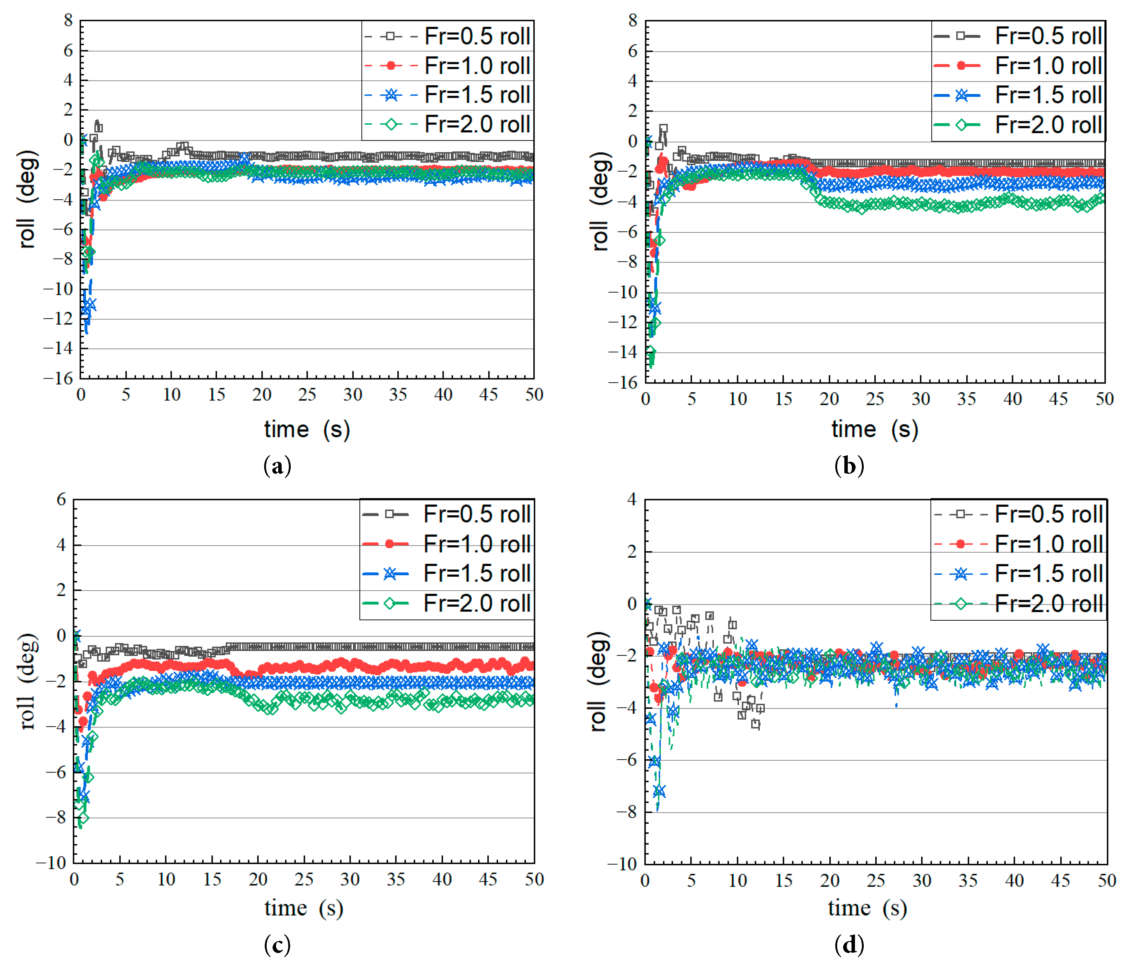
Figure 10: Roll response plots under different sea states and speeds. (a) Still water; (b) First-class sea state; (c) Second-class sea state; (d) Third-class sea state.
The maximum roll amplitude reached −15.36° at Sea State I and −7.83° at Sea State III, reflecting intensified hydrodynamic interactions under combined wave-speed excitation. The two key amplification mechanisms are: (1) reduced viscous damping due to decreased wetted surface area at Fr = 1.5, and (2) mismatch between wave encounter frequency and the craft’s natural roll frequency at higher speeds. The roll motion changes rapidly during (t = 0–2 s), and then gradually stabilizes. Sea State III causes over a threefold increase in roll amplitude compared to Sea State I, primarily due to nonlinear wave breaking and associated shock loading [12,13]. This nonlinear amplification becomes significant when wave height exceeds 0.8 m.
Key numerical observations: Calm water: Amplitude range −9.06° (Fr = 2.0) to −13.14° (Fr = 1.5), Sea state I: Peak amplitude −15.36° at Fr = 2.0 Sea state III: Minimum amplitude −7.83° at Fr = 2.0. The simulation results confirm the critical relationship between vessel speed, wave excitation energy, and transverse stability, offering quantitative references for defining the operational envelope of high-speed craft under varying sea conditions [31].
As illustrated in Fig. 11, the pitching response is observed at various speeds across four distinct sea states. It is evident that pitching amplitude is minimal in still water and increases progressively with sea state severity. In Sea State III, pitching motion is notably higher than in the other sea states, with both the magnitude and frequency of fluctuations significantly increased. As mentioned in Section 2.1, the design of this high-speed craft was based on the assumption that the Beaufort wind force did not exceed level 3. However, the pitching response shown in the Fig. 11d might be due to the fact that at level 3 sea conditions, the wind speed exceeded the design safety range of this high-speed craft. For instance, in Sea State III, the maximum longitudinal angle is 6.71° and the minimum is −14.47° at Fr = 0.5, while the minimum value further decreases to −18.03° at Fr = 2.0. In severe sea states, greater wave heights and wave lengths induce stronger undulatory forces in the longitudinal direction, leading to a marked increase in pitching. A trend similar to that of rolling is observed: pitching amplitude increases with Fr under constant sea state conditions. For example, an increase in Fr from 0.5 to 2.0 results in a pronounced rise in pitching amplitude in Sea State I, suggesting that speed is a key factor influencing pitching motion. The pitching response shows significant variation during the initial stage before stabilizing into a relatively consistent oscillation. However, the amplitude in this steady state is considerably higher in Sea State III.

Figure 11: Pitch response plots under different sea states and speeds. (a) Still water; (b) First-class sea state; (c) Second-class sea state; (d) Third-class sea state.
This may be attributed to the combined effects of increased wave height and energy, higher speed leading to resonance between the hull’s natural frequency and the wave encounter frequency, and a low hull aspect ratio contributing to reduced pitch and roll stability. The 0.8 m wave height exceeds the linear theory threshold (H/
Fig. 12 presents the heave response across different speeds for the four sea states. The figures show that heave amplitude increases markedly as sea state progresses from calm to Sea State III. In calm water (Fig. 12a), as Fr increases from 0.5 to 2.0, heaving amplitude grows from 0.06 m to 0.28 m, exhibiting a monotonic upward trend. Heaving remains minimal, and its variation across speeds is relatively smooth. Fig. 12b illustrates the heave response in Sea State I. Heave amplitude increases from 0.05 m at Fr = 0.5 to 0.29 m at Fr = 2.0, representing a faster rate of increase compared to calm water. In Sea State II (Fig. 12c), heave amplitude increases from 0.007 m at Fr = 0.5 to 0.082 m at Fr = 2.0—significantly higher than in Sea State I. The heave response in Sea State III (Fig. 12d) exhibits a substantial increase in amplitude and a noticeable acceleration in oscillation frequency, displaying clear periodic behavior. The amplitude grows from 0.012 m at Fr = 0.5 to 0.185 m at Fr = 2.0, indicating an exponential growth trend. Overall, vessel speed has a significant impact on the heave response. In general, the amplitude of heave oscillations increases with increasing speed and sea state severity.
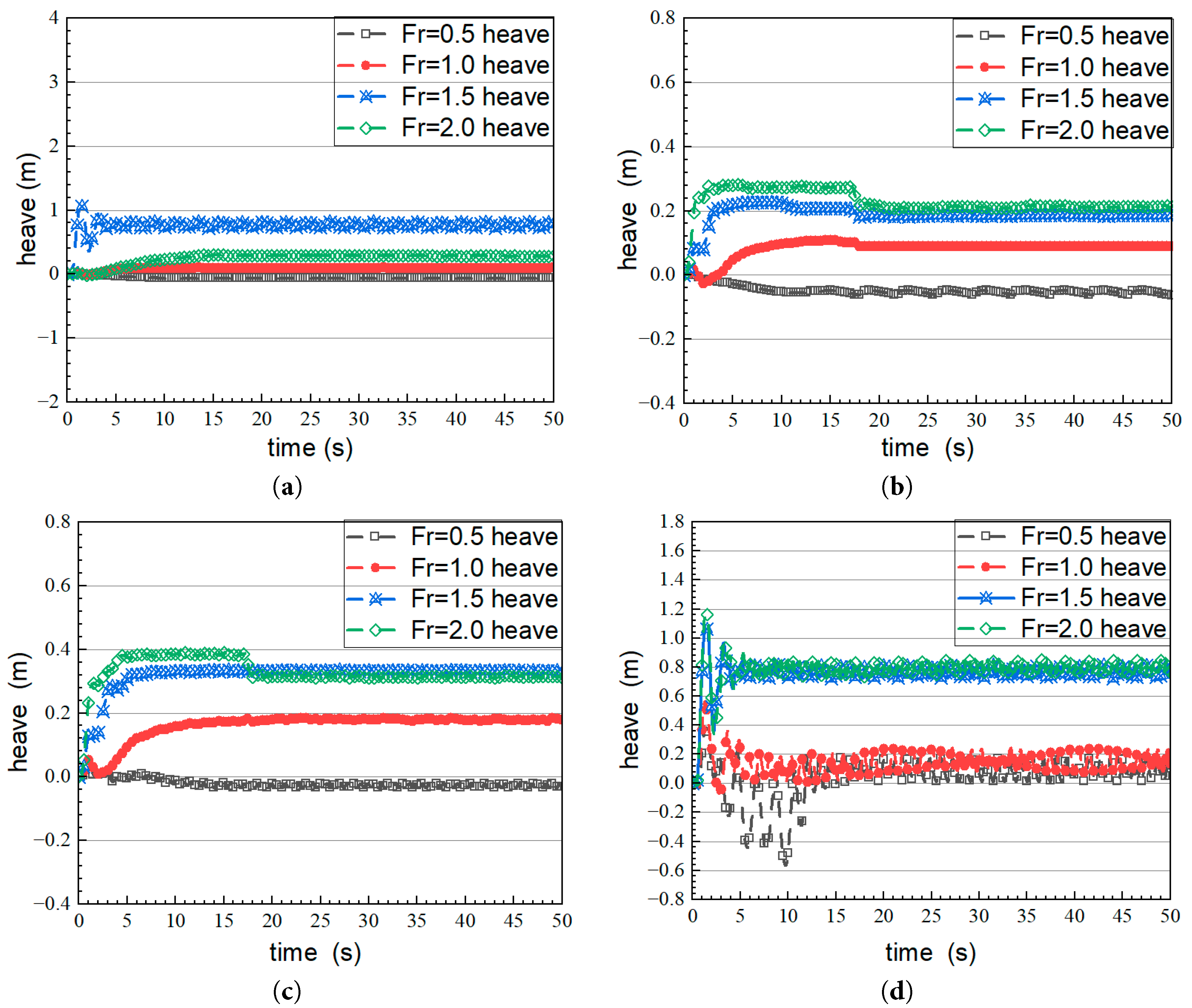
Figure 12: Heave response plots under different sea states and speeds. (a) Still water; (b) First-class sea state; (c) Second-class sea state; (d) Third-class sea state.
For example, in still water, as Fr increases from 0.5 to 2.0, the amplitude of heave motion gradually rises; a similar trend is observed in other sea states, indicating that high-speed sailing intensifies heave motion. In the initial stage of sailing, the heave response changes rapidly before gradually stabilizing into a relatively steady fluctuation. The time required to reach this steady state and the amplitude of stabilized oscillations vary across sea states and speeds. Under still water conditions without wave interference, viscous drag increases with speed, resulting in a continuous rise in the pitching response. In Sea State I (H = 0.055 m), wave effects are superimposed with the vessel’s bow wave, generating linear interference and amplifying the pitching response. In Sea State II (H = 0.3 m), nonlinear wave enhancement induces high-frequency shock loads, further increasing pitching response [29,30]. In Sea State III (H = 0.8 m), wave breaking and hull slamming trigger strong nonlinear responses. Simultaneously, violent heave oscillations cause dynamic variations in the wetted surface area, increasing nonlinear viscous damping.
As demonstrated in Fig. 13, the sway response varies with both speed and sea state. It is evident that sea state has a substantial influence on this response. In still water, sway displacement is minimal and varies gently. In Sea State I, displacement increases. In Sea State II, the oscillation trend becomes more pronounced. In Sea State III, the sway movement becomes complex, with increased displacement amplitude and more noticeable variation across speeds. As speed increases, the relationship between speed and oscillation response becomes non-monotonic. Even under the same sea state, speed significantly influences sway displacement. For instance, in still water, a higher Fr corresponds to a more pronounced sway trend. In a turbulent sea state such as Sea State III, the displacement at high speed (Fr = 2.0) is significantly greater than at Fr = 1.0. When Fr is below 1.0, the vessel is more sensitive to the wave’s low-frequency components, and higher sea states directly amplify wave forces, increasing hull hydrodynamic damping. However, when Fr exceeds 1.0, the damping effect of increased sea state diminishes. At the same time, nonlinear wave–hull interactions can lead to response saturation.

Figure 13: Sway response plots under different sea states and speeds. (a) Still water; (b) First-class sea state; (c) Second-class sea state; (d) Third-class sea state.
Fig. 14 shows the average values of total drag and thrust calculated for the high-speed craft under different sea states and speeds. As shown in Fig. 13a, the mean total drag doubles with increasing Fr under the same sea state. However, the rate of increase slows after Fr = 1.5 (e.g., only a 26% increase from Fr = 1.5 to 2.0 in Sea State III), which aligns with the phenomenon of drag saturation beyond the critical speed (Fr ≈ 1.2) predicted by Michell’s theory [27,29]. In still water, drag increases from 4542 N to 15,066 N (+232%) as Fr rises from 0.5 to 2.0. In Sea State I, it increases from 4590 N to 16,653 N (+263%), showing a significant nonlinear rise. The total drag also exhibits a generally monotonic increase with sea state class at the same Fr. However, at Fr = 2.0, drag in Sea State III (16,979 N) is 2.2% lower than in Sea State II (17,363 N). The drag increment is also 18% lower than the linear prediction at 60% wave breaking. This reduction is attributed to breaking waves dissipating approximately 30% of wave energy through vortices [15,16,17,18], thereby reducing effective drag. In addition, bow splash forms a gas-liquid mixing layer that reduces the wetted surface area by about 12%, decreasing frictional drag [25,29]. As shown in Fig. 13b, mean thrust gradually increases with Fr under the same sea state. In still water, thrust increases from 4544 N to 16,385 N (+260%) as Fr increases from 0.5 to 2.0, which agrees with the empirical formula P ∝ V3. Under the same Fr, peak thrust in Sea State I is observed at Fr = 1.5 (13,395 N), followed by a decrease at Fr = 2.0 (12,349 N). This trend is attributed to the limitations of the virtual disk model employed in this study, which represents propulsion as an idealized thrust source rather than a detailed propeller. Cavitation effects on propeller efficiency are not considered in this simplified model, as the virtual disk approximation overlooks blade geometry, unsteady flow interactions, and cavitation-induced performance degradation. The observed thrust reduction at higher Froude numbers reflects model simplifications rather than actual cavitation phenomena. Future research will incorporate detailed propeller modeling to address such physical mechanisms.

Figure 14: Mean values of drag and thrust for high-speed craft at various sea states and speeds. (a) Mean total resistance; (b) Mean thrust.
The mean thrust also increases monotonically with sea state class at a fixed Fr. At Fr = 1.0, thrust in Sea State III (10,623 N) is 22% higher than in still water, but at Fr = 2.0, the increase is only 2.1%, suggesting limited wave compensation capability at high speeds. The anomaly where mean thrust in Sea State III is lower than in Sea State I at Fr = 1.5 is likely due to sagging oscillations reaching approximately 0.8 m, which reduce the average propeller immersion depth by 0.3D (where D is the propeller diameter), thereby decreasing effective thrust [32].
The maneuverability considerations are based on heave and pitch responses. In Sea State III, heave amplitude exceeds 0.8 m, surpassing the craft’s 0.68 m design draft, violating safety limits. Meanwhile, pitch motions show extreme fluctuations (e.g., from 6.71° to −18.03° at Fr = 2.0), disrupting longitudinal stability. These excessive heave and pitch motions under severe sea states challenge the craft’s ability to maintain course and respond to control inputs, directly impacting maneuverability and safety—and considering maneuverability and safety—the following recommendations are proposed:
- (1)Sea state classification and control strategy:
- Still water and sea State I: A recommended speed range of Fr = 0.5–1.0. Rolling amplitude should be controlled within ±5°, heave swing displacement under 0.2 m, and drag growth kept linear. This supports both energy efficiency and passenger comfort.
- Sea State II: Maintain speed in the range of Fr = 1.0–1.5. Pitching response increases by approximately 40% compared to Sea State I and should be monitored closely, especially when heaving displacement exceeds 0.2 m due to the risk of deck wetting.
- Sea State III: The optimal speed is Fr = 1.0, with rolling controlled within −12°. This results in about a 35% increase in total resistance compared to still water. Ensuring sufficient engine power reserves is crucial.
- (2)Rolling-heaving mechanism:
- At Fr ≥ 1.5, the use of an active fin stabilizer system is recommended, as it can reduce rolling amplitude by 30–40% [20]. This system also mitigates the flapping phenomenon caused by roll–pitch coupling.
- In Sea State III, it is advisable to start operations at low speed (Fr = 0.5) and gradually increase to the target speed after stabilizing motion response (approximately five wave cycles).
In this paper, the six-degree-of-freedom motion characteristics of a high-speed craft in still water and under different sea state conditions are numerically investigated. The results reveal the coupling relationship between sea state parameters, speed, and the ship’s motion response. The main research conclusions are as follows:
- (1)The sea state level significantly affects the morphology of the free surface and the motion characteristics of the ship. As the sea state worsens (i.e., increased wave height, wave length, and wind speed), the free surface evolves from regular ship-generated waves to complex superimposed waves, with increased wave amplitude and more pronounced fragmentation. Correspondingly, the amplitudes of roll, pitch, heave, and sway increase significantly. For example, the maximum roll amplitude reaches −18.03° under the third-class sea state. The frequency of pitch oscillations also increases. As the sea state worsens, the stagnation point of the rooster-tail flow shifts aft, and the angle of the wake V-wave decreases.
- (2)The Fr value directly influences the motion amplitude by altering the interaction frequency between the hull and waves. In still water and low sea states, motion amplitudes (roll, pitch, heave, and sway) are minimized at Fr = 0.5. In third-class sea conditions, a speed corresponding to Fr = 1.0 effectively suppresses motion amplitudes. When Fr approaches the critical value (e.g., Fr = 2.0), resonance may occur due to alignment between the hull’s natural frequency and the wave encounter frequency, leading to a sharp increase in drag and motion instability.
- (3)At a constant Fr, total resistance increases monotonically with worsening sea state, with resistance in the third-class sea state more than 30% higher than in still water. Thrust demand also rises significantly with increasing speed, due to the greater impact and disturbance of waves on the hull. This results in higher average thrust requirements to maintain sailing speed under rougher conditions.
- (4)The initial sailing phase is characterized by intense motion responses.
The intense initial motion responses (roll, pitch, sway, heave), especially at Fr = 2.0, partly from the idealized virtual disk propulsion model. This model approximates thrust uniformly without propeller dynamics, potentially causing unphysical transient forces during rapid acceleration. However, observed transients also reflect valid hydrodynamic memory effects (Lewandowski [1]) like added mass and radiation damping. These physical phenomena inherently cause lag between hull forces and motion, generating transients before steady state, independent of numerical initialization. Thus, the responses combine model limitations with real fluid dynamics.
Under rough sea conditions, it is recommended to start at low speed to minimize transient impacts. For medium and high sea states, a speed corresponding to Fr = 1.0 is recommended to balance stability and efficiency.
Acknowledgement:
Funding Statement: This work was funded by the National College Students Innovation and Entrepreneurship Training Program (202411646031), the Zhejiang Xinmiao Talents Program (2024R405A052), and the SRIP Research Program of Ningbo University (2025SRIP1707).
Author Contributions: The authors confirm contribution to the paper as follows: study conception and design: Xiaoyang Wu, Wenchao Han; data collection: Xinqi Wang; analysis and interpretation of results: Wenchao Han, Min Kuang; graphics and curves: Xinqi Wang; draft manuscript preparation: Xiaoyang Wu, Wenchao Han, Wenhao Xie. All authors reviewed the results and approved the final version of the manuscript.
Availability of Data and Materials: The data that support the findings of this study are available from the Corresponding Author, Min Kuang, upon reasonable request.
Ethics Approval: Not applicable.
Conflicts of Interest: The authors declare no conflicts of interest to report regarding the present study.
References
1. Lewandowski EM. The dynamics of marine craft: maneuvering and seakeeping. Vol. 22. Singapore: World Scientific Publishing; 1995. [Google Scholar]
2. Savitsky D. Hydrodynamic design of planing hulls. Mar Technol SNAME News. 1964;1(4):71–95. doi:10.5957/mt1.1964.1.4.71. [Google Scholar] [CrossRef]
3. Griffin OM. Ship wave modification by a surface current field. J Ship Res. 1988;32(3):186–93. doi:10.5957/jsr.1988.32.3.186. [Google Scholar] [CrossRef]
4. Shiryaeva M, Subbotina M, Subbotin S. Linear and non-linear dynamics of inertial waves in a rotating cylinder with antiparallel inclined ends. Fluid Dyn Mater Process. 2024;20(4):787–802. doi:10.32604/fdmp.2024.048165. [Google Scholar] [CrossRef]
5. Blount DL, Codega LT. Dynamic stability of planing boats. Mar Technol SNAME News. 1992;29(1):4–12. doi:10.5957/mt1.1992.29.1.4. [Google Scholar] [CrossRef]
6. Li S, Zhong WA, Yu S, Wang H. Numerical study of cavitating flows around a hydrofoil with deep analysis of vorticity effects. Fluid Dyn Mater Process. 2025;21(1):179–204. doi:10.32604/fdmp.2024.056228. [Google Scholar] [CrossRef]
7. Yasukawa H, Hirata N, Nakayama Y. High-speed ship maneuverability. J Ship Res. 2016;60(4):239–58. doi:10.5957/jsr.2016.60.4.239. [Google Scholar] [CrossRef]
8. Belga F, Ventura M, Guedes Soares C. Seakeeping optimization of a catamaran to operate as fast crew supplier at the Alentejo basin. In: Progress in maritime technology and engineering. Boca Raton, FL, USA: CRC Press; 2018. p. 587–97. doi:10.1201/9780429505294-66. [Google Scholar] [CrossRef]
9. Shi KY, Zhu RC. A fully nonlinear approach for efficient ship-wave simulation. J Hydrodyn. 2023;35(6):1027–40. doi:10.1007/s42241-024-0092-9. [Google Scholar] [CrossRef]
10. Takami T, Kitahara M, Jensen JJ, Matsui S. Extreme nonlinear ship response estimations by active learning reliability method and dimensionality reduction for ocean wave. Mar Struct. 2025;99:103723. doi:10.1016/j.marstruc.2024.103723. [Google Scholar] [CrossRef]
11. Wu Z, Zhou B, Wang Y, Jin G, Liu H, Zhang T. A 3D TEBEM for simulating time domain motions of ships in waves with forward speed considering the effects of ship wave. Ocean Eng. 2025;317:119996. doi:10.1016/j.oceaneng.2024.119996. [Google Scholar] [CrossRef]
12. Tavakoli S, Dashtimanesh A. A six-DOF theoretical model for steady turning maneuver of a planing hull. Ocean Eng. 2019;189:106328. doi:10.1016/j.oceaneng.2019.106328. [Google Scholar] [CrossRef]
13. Park S, Wang Z, Milano C, Stern F, Gunderson A, Scherer J, et al. 6DoF CFD analysis for high-speed small craft in free running conditions. Ships Offshore Struct. 2024:1–21. doi:10.1080/17445302.2024.2393478. [Google Scholar] [CrossRef]
14. Cao H. Research on the calculation of resistance of skiff based on Fluent. J Hydrodyn. 2008;20(S1):156–61. (In Chinese). [Google Scholar]
15. Shen H, Chen Q, Su Y. Research on the numerical prediction method of three-dimensional hydrodynamic power of taxiing boat based on CFD technology. In: Proceedings of the 15th China Ocean (Onshore) Engineering Symposium; 2011; Qingdao, China. Beijing, China: China Ocean Engineering Society; 2011. p. 207–11. [Google Scholar]
16. Yao J, Cheng X, Song X, Zhan C, Liu Z. RANS computation of the mean forces and moments, and wave-induced six degrees of freedom motions for a ship moving obliquely in regular head and beam waves. J Mar Sci Eng. 2021;9(11):1176. doi:10.3390/jmse9111176. [Google Scholar] [CrossRef]
17. Yu Z, Amdahl J. Full six degrees of freedom coupled dynamic simulation of ship collision and grounding accidents. Mar Struct. 2016;47:1–22. doi:10.1016/j.marstruc.2016.03.001. [Google Scholar] [CrossRef]
18. Menter FR. Two-equation eddy-viscosity turbulence models for engineering applications. AIAA J. 1994;32(8):1598–605. doi:10.2514/3.12149 [Google Scholar] [CrossRef]
19. Nanda MI, Purnamasari D, Baidowi A, Syarif IS. Verification and validation of ITTC benchmark ship CFD performance towards development of CFD and EFD combined methods. IOP Conf Ser Earth Env Sci. 2023;1198(1):012027. doi:10.1088/1755-1315/1198/1/012027. [Google Scholar] [CrossRef]
20. Andrun M, Blagojević B, Bašić J. The influence of numerical parameters in the finite-volume method on the Wigley hull resistance. Proc Inst Mech Eng Part M J Eng Marit Envrion. 2019;233(4):1123–32. doi:10.1177/1475090218812956. [Google Scholar] [CrossRef]
21. Siemens. STAR-CCM+ Documentation. Siemens Digital Industries Software. Munich, Germany: Siemens; 2023. [Google Scholar]
22. Issa RI. Solution of the implicitly discretised fluid flow equations by operator-splitting. J Comput Phys. 1986;62(1):40–65. doi:10.1016/0021-9991(86)90099-9. [Google Scholar] [CrossRef]
23. Al-Faifi S. Toward the development of a comprehensive nuclear system analysis code based on two-fluid model: starting with an isentropic approach. Arab J Sci Eng. 2025;50(5):3533–8. doi:10.1007/s13369-024-09709-9. [Google Scholar] [CrossRef]
24. Zou J, Sun H, Ji P. Influence of mesh on resistance calculation of trimaran planing hulls. Ship and Boat. 2016;27(3):8–14. (In Chinese). doi:10.3969/j.issn.1001-9855.2016.03.002. [Google Scholar] [CrossRef]
25. Patankar S. Numerical heat transfer and fluid flow. Boca Raton, FL, USA: CRC Press; 2021. doi:10.1201/9781482234213. [Google Scholar] [CrossRef]
26. Ubbink O, Issa RI. A method for capturing sharp fluid interfaces on arbitrary meshes. J Comput Phys. 1999;153(1):26–50. doi:10.1006/jcph.1999.6276. [Google Scholar] [CrossRef]
27. Yang D, Sun Z, Jiang Y, Gao Z. A study on the air cavity under a stepped planing hull. J Mar Sci Eng. 2019;7(12):468. doi:10.3390/jmse7120468. [Google Scholar] [CrossRef]
28. ITTC. Uncertainty analysis in CFD verification and validation [Internet]. 2008 [cited 2025 Aug 1]. Available from: https://www.ittc.info/media/11950/75-03-01-01.pdf. [Google Scholar]
29. Faltinsen O. Sea loads on ships and offshore structures. Cambridge, UK: Cambridge University Press; 1990. doi:10.1146/annurev.fluid.22.1.35. [Google Scholar] [CrossRef]
30. Deng R, Huang S, Wang S, Liu H, Yu X, Wu T. Experimental study on the influence of a T-foil and bulbous bow on the resistance and motion in regular head waves of trimarans. Ocean Eng. 2023;281:114990. doi:10.1016/j.oceaneng.2023.114990. [Google Scholar] [CrossRef]
31. Wang H, Zhu R, Zha L, Gu M. Experimental and numerical investigation on the resistance characteristics of a high-speed planing catamaran in calm water. Ocean Eng. 2022;258:111837. doi:10.1016/j.oceaneng.2022.111837. [Google Scholar] [CrossRef]
32. Sheng Z. Ship principle. Shanghai, China: Shanghai Jiaotong University Press; 2017. (In Chinese). [Google Scholar]
Cite This Article
 Copyright © 2025 The Author(s). Published by Tech Science Press.
This work is licensed under a Creative Commons Attribution 4.0 International License , which permits unrestricted use, distribution, and reproduction in any medium, provided the original work is properly cited.
 Downloads
 Citation Tools