CFD Simulation of Passenger Car Aerodynamics and Body Parameter Optimization

1 Introduction

1.1 Necessity of the Study

As the global ownership of new energy vehicles increases, the need to reduce air resistance becomes more evident to decrease resource waste. During operation, vehicles are affected by two main types of external resistance: air resistance and rolling resistance. When the vehicle speed reaches a certain level, the proportion of air resistance in the total external resistance increases sharply, leading to an increase in vehicle battery power consumption [1]. By effectively reducing resistance, it is possible to improve the vehicle’s stability, handling, economy, and other aerodynamic-related performance. The dynamic characteristics of the vehicle’s external flow field directly affect the assessment of vehicle comfort. Therefore, automotive companies attach great importance to aerodynamic simulation analysis of vehicles, and to improve the aerodynamic performance of the automotive industry, they have invested significant manpower, material, and financial resources. Traditional studies on vehicle aerodynamics are mainly based on wind tunnel experiments, which require a large initial investment and are time-consuming. Thus in recent years, with the increased development of computers and continuous progress in turbulence theory, the CFD method has been widely applied and utilized in the study of vehicle aerodynamic performance.

By using advanced numerical simulation methods, it is possible to analyse and study the flow field characteristics of vehicles more effectively. Moreover, by combining traditional methods, it is possible to significantly improve the aerodynamic performance of vehicles, increase the efficiency of CFD, and reduce research and development costs. Reasonable aerodynamic performance is crucial for improving a vehicle’s power, economy, and other performance metrics. Therefore, while optimizing aerodynamic characteristics, it is essential to consider how the design can also fulfil manufacturing feasibility and engineering constraints in real-world vehicle development.

This study divides the vehicle into front, middle, and rear parts for separate research. The front part includes the hood angle (α) and windshield angle (β), the rear part includes the rear windshield angle (γ) and rear upwards tail lift angle (θ), and the middle part mainly includes the ground clearance (d) and the side angle of the body (s). By studying these different angles and ground clearances, the optimal aerodynamic drag coefficient C d can be determined.

1.2 Previous Research

Alkan et al. [2] conducted CFD simulations to investigate the aerodynamic performance of a sedan under different diffuser angles. Their study revealed that as the diffuser angle increased, the drag coefficient decreased until an optimal point around 7°, beyond which flow separation intensified, leading to increased drag and reduced aerodynamic efficiency. Qin et al. [3], through CFD simulation and wind tunnel testing, analysed the aerodynamic performance of a 1:4 scale DrivAer notchback model and reported that the hybrid RANS-LES method strikes a good balance between accuracy and cost-effectiveness and provides guidance for optimized mesh generation. Rostamzadeh-Renani et al. [4] studied the reduction in vehicle drag and lift by designing and optimizing roof spoilers, resulting in performance optimisations of 21.27% and 19.91%, respectively. Le Good et al. [5] analysed the wind resistance effect of different shaped vehicles in formation driving through wind tunnel testing and reported that the optimal shape of a vehicle depends on its position within the formation. Vignesh et al. [6] studied the impact of the windshield angle on drag using ANSYS Fluent for CFD analysis with an inlet speed of 20 m/s and found varying drag coefficients by adjusting the windshield angle and speed. Song et al. [7] utilized artificial neural networks for aerodynamic optimization of the rear shape of sedans, improving performance by approximately 5.64%, which could enhance fuel efficiency for sedans, with the benchmark model being the Hyundai Motor Company’s YF SONATA. Huminic and Huminic [8] research indicated that bodies with curved diffusers perform better aerodynamically than those with flat bottom diffusers do, offering significantly increased downforce, reduced drag, and various advantages in vehicle design. Widodo and Karohmah [9] used CFD to study rear diffuser angles on a bus model and found that a 12° diffuser provided optimal drag reduction (2.3%) and improved stability. Bayındırlı and Çelik [10] showed that increasing windshield inclination from 0° to 45° reduced drag by up to 17.92%, with high sensitivity to angle changes. Chen et al. [11] introduced TripNet, a triplane deep learning model, which accurately predicted drag and flow fields with lower computational cost. Valencia and Lepin [12] demonstrated that standard and curved diffusers could reduce drag by up to 10% and significantly lower lift between 60–120 km/h. Buscariolo et al. [13] found that for Ahmed bodies, a 30° diffuser worked best on a 0° slant, while a 20° diffuser was optimal for 25° slant configurations. Abdellah and Wang [14] applied ANSYS-based CFD and found that optimal windshield angles significantly reduce aerodynamic drag, highlighting the impact of front geometry on vehicle performance. Although previous studies have extensively analysed the effects of individual vehicle components—such as diffusers, windshields, roof spoilers, and underbody configurations—on aerodynamic performance, these works often isolate single variables and do not offer comprehensive optimization across multiple body zones. Moreover, few studies have systematically compared front, middle, and rear design parameters under consistent simulation conditions. This study aims to bridge this gap by simultaneously examining the influence of multiple parameters across different body regions on the overall drag coefficient ( C d ) via a unified CFD approach. This provides a more integrated understanding of how combined design changes affect aerodynamic efficiency, which has not been sufficiently explored in previous studies.

1.3 Optimization of the Aerodynamic Characteristics of Automobile Bodies

In modern automotive design, the importance of aerodynamic performance is increasingly emphasized [15]. Aerodynamic design can not only improve fuel efficiency but also enhance vehicle handling and stability. With technological advancements, automobile manufacturers are continuously exploring ways to reduce air resistance by optimizing the shape of the vehicle body and component design. The C d is one of the key indicators for measuring a vehicle’s aerodynamic performance. Previous studies have focused mostly on the impact of a single part or angle on the C d , whereas this study divides the car into front, middle, and rear sections for a more comprehensive and detailed investigation. Therefore, through a series of numerical simulations and experimental tests, this study analyses the impact of parameters such as the angle of the front windshield, the angle of the hood, the angle of the rear window, and the ground clearance on the C d value.

1.4 Novelty and Contributions

The novelty of this study lies in its systematic, region-based parametric investigation of vehicle aerodynamic performance. Unlike previous works that typically examine the influence of a single geometric feature in isolation, we propose a comprehensive optimization framework that divides the car body into three functional sections—front, middle, and rear—and evaluates the combined effects of multiple design angles (such as the hood angle, windshield inclination, rear window angle, ground clearance, and side edge angle) on the drag coefficient ( C d ). Using STAR-CCM+ simulations, this study reveals new insights into the interaction of these parameters and provides practical guidelines for holistic vehicle body optimization. This integrative approach enhances both the aerodynamic efficiency and feasibility of design implementation, which has not been sufficiently addressed in the literature.

2 Theoretical Analyses

2.1 Governing Equations

In this study, the flow around a vehicle is modelled using the Reynolds-averaged Navier‒Stokes (RANS) equations, which are appropriate for high-Reynolds-number turbulent flows over bluff bodies such as cars. The standard RANS formulation, together with a two-equation turbulence model, allows for a reasonable balance between computational efficiency and accuracy. The governing equations include the continuity equation, the momentum equation, and two additional transport equations for turbulence modelling.

Their mathematical expressions are as follows.

Dominant Equation

Turbulence Kinetic Energy Equation

Momentum Balance Equation

Dissipation Equation

Turbulent Viscosity Coefficient μt=ρCμk2ε(5) where “ ρ ” is fluid density, p is the pressure, u i represents the velocity component in the i direction, x i is the spatial coordinate, k is turbulent kinetic energy, ε is the turbulent dissipation rate, μ is dynamic viscosity, μ t is turbulent viscosity, τ is the viscous stress, τRe is the Reynold sturbulent stress (which depends on the turbulent viscosity), σ k is the Prandtl number, G k is production of turbulent kinetic energy due to mean velocity gradients, σ ε is turbulent Prandtl number for ε.

The governing equations of fluid flow, including the continuity, momentum, and turbulence transport equations used in this study, are based on the Reynolds-averaged Navier‒Stokes (RANS) formulation, which is widely adopted in CFD for engineering applications [16,17].

2.2 Resistance

The aerodynamic resistance is modelled using the standard pressure drag formulation suitable for external flows [18]. Since the focus is on macroscale drag over a full car body, no empirical porous or Darcy–Forchheimer-type drag laws are applied. The drag force is calculated on the basis of the surface integration of pressure and shear stress over the vehicle body via the standard formulation for the drag coefficient:

Drag is the resistance force encountered by an object in motion. The drag on a car depends on the frontal area of the vehicle. Compared with those with streamlined bodies, vehicles with larger frontal areas experience more pressure drag.

The equation for resistance is as follows:

This method is consistent with established practices in vehicle external aerodynamics CFD modelling [19].

To close the RANS equations, the standard k-ε turbulence model is employed due to its balance between computational efficiency and acceptable accuracy for engineering turbulent flows. Although alternative models such as SST k-ω or RNG k-ε may offer improved performance in specific scenarios, the standard model remains a robust choice for general applications.

2.3 Turbulence Model

The standard k-ε turbulence model, originally proposed by Launder and Spalding, is used in this study. This model is widely applied in engineering applications because of its simplicity and robustness. Although it may not capture all the complex turbulent structures in highly separated flows, it provides sufficiently accurate predictions for the external aerodynamics of road vehicles under steady-state conditions [18]. Compared with more advanced models such as the SST k-ω or hybrid LES/RANS methods, the standard k-ε model significantly reduces the computational cost while still producing reliable trends in drag coefficient variation for parametric studies.

The Navier‒Stokes equations are nonlinear second-order partial differential equations. Therefore, while it is possible to directly solve the N‒S equations for turbulence numerically, traditional computational resources are insufficient to address the complex turbulence problems involved in engineering. In such cases, turbulence modelling is typically used to solve the Reynolds-averaged Navier‒Stokes equations. The core idea is to decompose the excessive terms in the N‒S equations into time-averaged and fluctuating components. Owing to the introduction of turbulent components, inferring the effects of turbulent flow from the mean flow alone is impossible, necessitating the construction of turbulence models to close the equations [20]. The standard k-ε model was selected for the numerical simulation of the vehicle’s external flow field. When the fluid enters the computational domain through the inlet, outlet, or far-field boundary, it is necessary to specify the turbulence intensity to ensure that the turbulence conditions at the boundaries closely match the actual scenario. This helps to avoid impacting the computation results and causing divergence. In this study, the flow around the vehicle occurs at a Reynolds number on the order of 10 − 7 , as calculated on the basis of the vehicle length and inlet velocity. This high Reynolds number indicates fully turbulent external flow, which justifies the use of Reynolds-Averaged Navier‒Stokes (RANS) turbulence modelling. The specific turbulence parameters are set as follows:

• (1)The Reynolds number (Re) is defined as:

In the equation, L represents the characteristic length, which in this study is taken as the wheelbase of the vehicle.

• (2)Turbulence intensity I:

In the equation, u′ represents the fluctuating velocity, and u a v g denotes the mean velocity, i.e., the inlet flow velocity.

• (3)Turbulent kinetic energy k:

• (4)Turbulent kinetic energy dissipation rate ε:

In the equation, l represents the turbulence length scale, which is typically taken as 0.07 times the hydraulic diameter of the computational domain. The hydraulic diameter is defined as four times the ratio of the inlet area to the perimeter of the computational domain. After the boundary conditions and turbulence parameters are set, the SIMPLE pressure‒velocity algorithm is employed for steady-state calculations via a pressure-based solver. In this study, the standard k-ε turbulence model is employed because of its robustness and efficiency in external aerodynamic flow simulations.

2.4 Boundary Layer Treatment

In turbulent flow near solid boundaries, the wall exerts a dominant influence on both the mean flow and the turbulence. Accurate boundary layer treatment is essential, particularly in external aerodynamics. In this study, a wall function approach is adopted to model the near-wall region, which provides a practical balance between computational cost and accuracy for high-Reynolds-number flows.

Compared with wall-resolved models, which require very fine meshes (especially in the viscous sublayer), wall functions apply semiempirical relations to bridge the wall and the turbulent core, assuming that the first grid layer lies within the logarithmic region of the boundary layer (typically for 30 < y + < 300 ).

As shown in Fig. 1, the y + values in our mesh range from 0100, with most values being approximately 50, indicating that the mesh resolution is appropriate for wall function-based treatment. This strategy significantly reduces mesh complexity while maintaining acceptable accuracy in capturing aerodynamic effects along the vehicle surface.

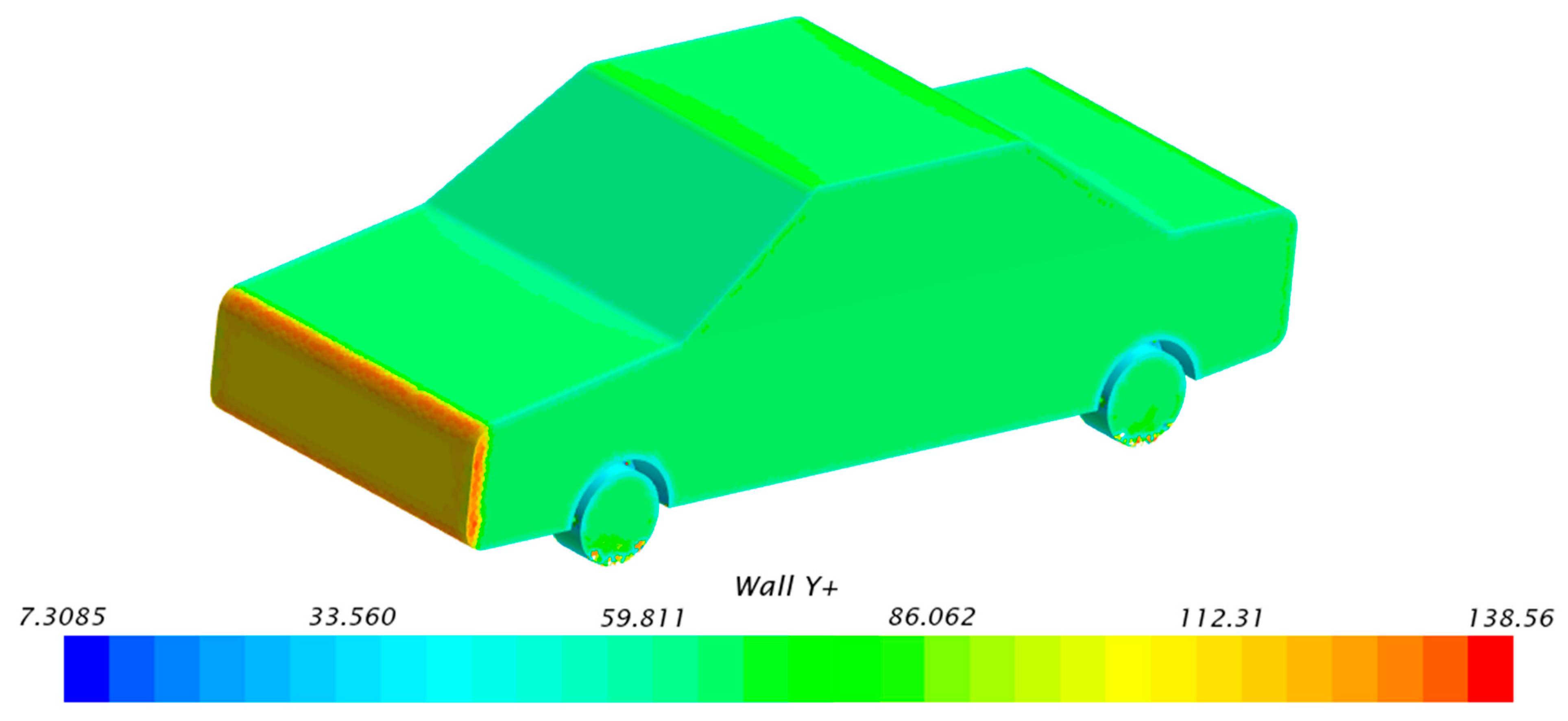
Figure 1: Vehicle body wall y+ distribution contour map.

Table 1 summarizes the key differences between wall-resolved and wall-function approaches in CFD, highlighting their respective mesh requirements, computational costs, and suitability for external aerodynamic applications such as vehicle design.

The presence of walls has a significant impact on turbulent flow, serving as a major source for both mean flow and turbulence. At the wall, the mean velocity field must satisfy the no-slip condition, whereas in the boundary layer region, viscous damping reduces fluctuations in the tangential velocity, and the presence of the wall prevents the normal fluctuations of turbulence, making the treatment of the boundary layer critical to the computational results. Typically, the boundary layer is roughly divided into three layers. The middle layer is referred to as the “viscous sublayer”, where the flow is dominated by laminar flow; the outermost layer is known as the “logarithmic layer”, where turbulence plays a primary role; and the intermediate region between the viscous sublayer and logarithmic layer is called the “transition layer”, where both molecular viscosity and turbulence effects are significant. There are two approaches for handling the boundary layer: wall models and wall functions. The wall model approaches handle the boundary layer on the basis of the turbulence model, requiring a more refined mesh and relatively higher computational costs. The wall function approaches do not solve the boundary layer through turbulence but use empirical formulas, or wall functions, to connect the flow at the wall to the turbulent core region. In CFD simulations, it suffices to place the first grid layer node within the logarithmic layer, meaning that the thickness of the first grid layer is less than y. This paper adopts the wall function approach to simulate the aerodynamic characteristics of the car body [20,21].

3 CFD Modelling

3.1 CFD Software and Setup

The CFD simulations in this study were conducted using STAR-CCM+ (Version 2022.1, Siemens Digital Industries Software). This software integrates CAD modelling, meshing, physics setup, and post processing within a single environment, which streamlines the aerodynamic simulation workflow.

The physical model was constructed and imported into STAR-CCM+, followed by mesh generation using the built-in Polyhedral Mesher with Prism Layer refinement for near-wall accuracy. The segregated flow solver was employed under steady-state conditions with the standard k-ε turbulence model. All the simulations used double precision to improve the solution stability and accuracy.

3.2 Model Analysis

3.2.1 Physical Model

The vehicle model used in this study is a simplified sedan-type passenger car designed to resemble the geometric features of modern electric vehicles while ensuring computational efficiency. The model was constructed using CAD software on the basis of typical dimensions of mid-size sedans, with modifications to allow parametric variation in key aerodynamic features such as hood angle, windshield inclination, rear window slope, ground clearance, and side body curvature.

The model is not based on a commercial vehicle but rather on a generic shape inspired by previous studies on external vehicle aerodynamics (e.g., the DrivAer model [3] and SAE models [22]), which are tailored to support systematic parametric analysis. This choice allows better control of geometry for CFD studies without the complexity of full production-car details (e.g., underbody roughness, mirrors, or grilles).

The vehicle has the following dimensions: 4200 mm in length, 1600 mm in width, 1400 mm in height, and a wheelbase of 2700 mm. It features smooth contours and a symmetric body design to focus the analysis on major surface angles. The model omits fine details such as door gaps and tires to reduce the computational cost and mesh complexity.

A 3D view of the base vehicle model is shown in Fig. 1 and Table 2, which illustrates the overall shape and major variable parameters. This base model supports controlled studies of how geometry influences aerodynamic drag under steady-state, high-Reynolds-number flow conditions.

3.2.2 Verifying the Simulation Results

After the simulation, the Wall Y plus (y+) contour map around the vehicle body is examined, as shown in Fig. 1. The y+ values around the vehicle body fluctuate between 0 and 100, with the y+ values in most areas of the vehicle body being approximately 50, indicating that the treatment of the near-wall region of the vehicle body in this study is reasonable.

3.2.3 Fluid Domain Model

The computational domain for this study is defined as follows: the distance from the rear of the car to the domain inlet is four times the car length, and the distance from the rear of the car to the domain outlet is six times the car length, resulting in a total domain length of ten times the car length. The distance from each side of the car to the corresponding sides of the domain is 1.5 times the car width, with a total domain width of four times the car width. The distance from the car roof to the top boundary of the domain is five times the car height, and the total domain height is six times the car height. The computational domain and car body model used in this study are illustrated in Fig. 2.

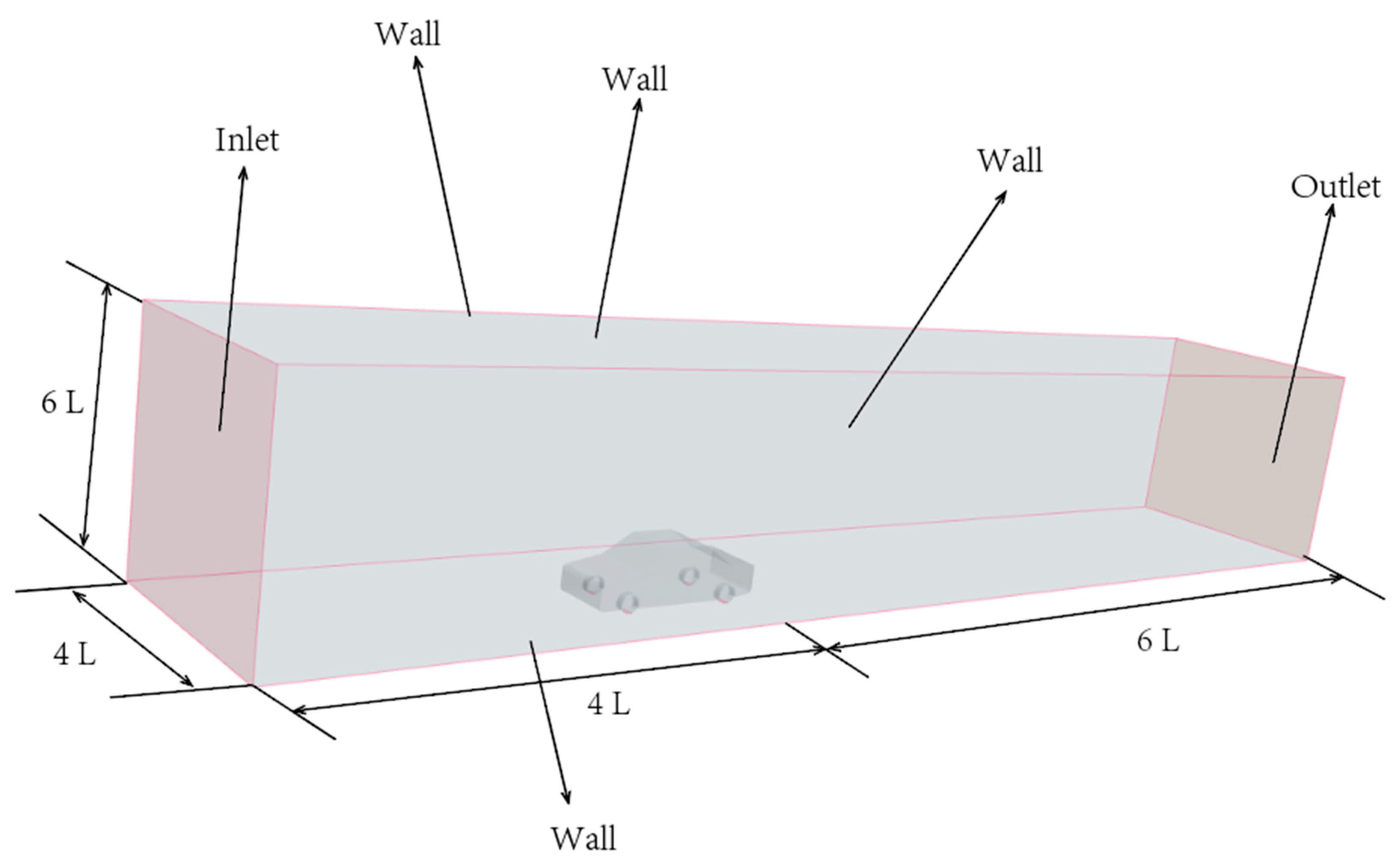
Figure 2: CFD computational domain.

The dimensions of the computational domain were determined on the basis of best practices in external vehicle aerodynamics simulations. Specifically, the inlet boundary was placed 4 times the vehicle length upstream, and the outlet boundary was set 6 times the vehicle length downstream to minimize backflow and wake reflection. The lateral boundaries were positioned 1.5 times the vehicle width from either side, and the vertical domain was extended to 6 times the vehicle height.

These settings ensure that the artificial boundaries do not interfere with the natural development of the wake and pressure fields. Similar domain configurations have been successfully used in prior aerodynamic studies of passenger vehicles [20].

The computational domain was constructed to minimize the influence of boundary conditions on the flow around the vehicle. In accordance with established guidelines for external vehicle aerodynamics simulations [19], the inlet boundary was set at a distance of 4 times the vehicle length upstream of the car, and the outlet was located 6 times the vehicle length downstream. The lateral boundaries were placed at 1.5 times the vehicle width on either side, and the domain height was set to 6 times the vehicle height. These settings ensure that pressure waves and wake effects are not artificially reflected from the boundaries, thus preserving the physical realism of the simulated flow.

3.2.4 y+ Assessment and Near-Wall Mesh Quality

To ensure compatibility between the turbulence model and near-wall mesh resolution, the nondimensional wall distance ( y + ) was evaluated across the vehicle surface after meshing. Since this study employs the standard k-ε turbulence model with wall functions, it is crucial that the first layer of mesh cells falls within the logarithmic region of the boundary layer (typically 30 < y + < 300 ).

As shown in Fig. 3, the majority of y + values fall between 30 and 100, with most surface regions averaging approximately 50. This confirms that the mesh resolution near the wall is appropriate for the wall-function-based approach, allowing accurate representation of the near-wall shear stress without requiring excessive mesh refinement. Areas with slightly lower y + values (e.g., around stagnation points) are limited and do not significantly affect the overall simulation accuracy.

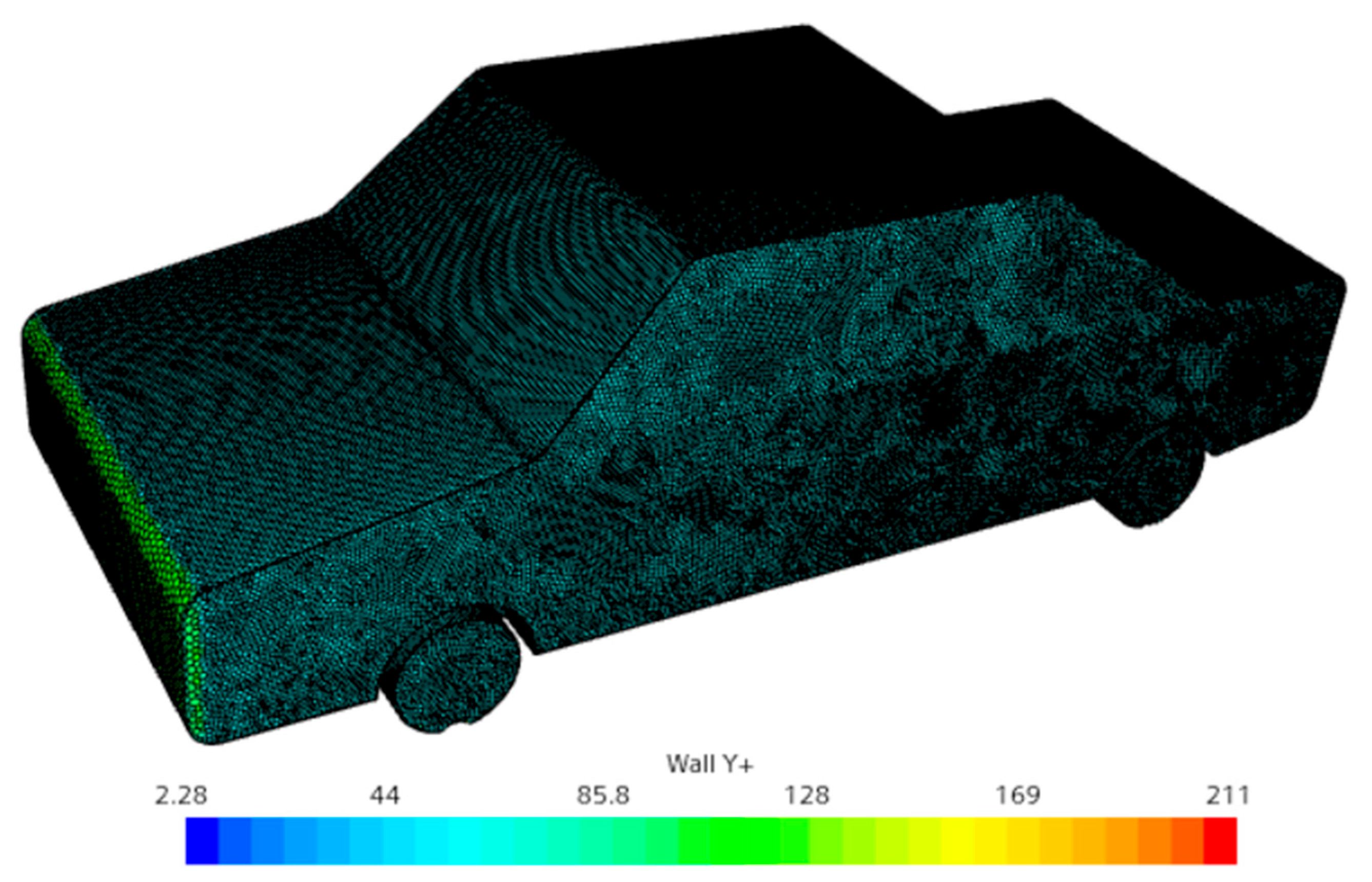
Figure 3: Distribution of wall distance y +  over the vehicle surface.

Most surface regions maintain y + within the recommended range for wall function modelling, ensuring compatibility with the standard k-ε turbulence model.

3.3 CFD Fluid Mechanics Analysis

3.3.1 Mesh Setting

In computational fluid dynamics (CFD) and other simulation fields, meshing refers to the process of dividing a continuous physical domain (such as fluid or solid) into discrete small cells or elements for numerical computation. The primary function of meshing is to transform complex geometries and flow features into a form that can be discretely processed, allowing numerical solvers to approximate the solution of flow equations within these small cells. As shown in Table 3, contains the types of mesh and their polyhedral parameters.

To simulate the aerodynamic performance of passenger vehicles accurately, this study employs CFD methods and carries out detailed mesh setting. A combination of structured and unstructured grids was used to generate finer meshes around the vehicle’s complex geometry. The meshing process was carried out using the built-in meshing tools of STAR-CCM+. During the CFD analysis, meshes were created on both the vehicle domain and the surrounding fluid domain. Over-refining the tunnel mesh can reduce the accuracy of the analysis; therefore, generating meshes of appropriate size is crucial. In this study, the mesh size around the vehicle’s complex flow field was set to one-eighth of the tunnel mesh size to ensure an appropriate grid resolution. The mesh size around the vehicle was set to 0.05 m, whereas the tunnel mesh size was 0.5 m. A total of 1,476,079 cells were created. The Prism Layer Mesher was employed to capture the viscous flow near the walls in greater detail, whereas the Trimmer was used to interpret the mesh in rectangular shapes.

3.3.2 Mesh Independence Analysis

Mesh independence studies are essential in CFD to ensure that numerical results are not significantly affected by the discretization resolution. They constitute a critical part of the overall uncertainty quantification (UQ) process in numerical simulations [23]. According to best practices, numerical uncertainty due to grid size should be minimized or quantified through systematic mesh refinement, especially when sensitive aerodynamic parameters such as the drag coefficient ( C d ) are predicted.

In this study, five different mesh configurations were tested, ranging from 215,896 to 1,749,884 cells. The variation in the computed C d values was monitored to assess convergence. As shown in Fig. 4, the relative difference in C d between Mesh 3 (1.13 million cells) and Mesh 4 (1.47 million cells) was less than 3%, indicating acceptable mesh independence for engineering accuracy. Although a formal grid convergence index (GCI) evaluation was not performed, the observed convergence trend is consistent with prior recommendations for external vehicle aerodynamics [24].

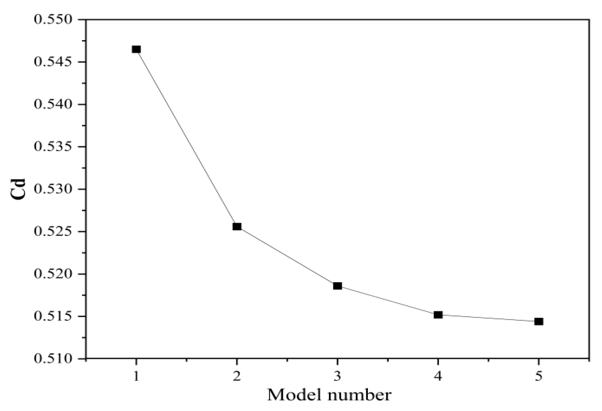
Figure 4: Mesh independence analysis.

3.3.3 Analysis Results

The physical conditions are set as shown in Table 4 below:

The boundary conditions are shown in Table 5 and Table 6. The vehicle remains stationary, the flow inlet region is set to a uniform velocity of 30.56 m/s, the outlet is set to a constant pressure, and the side faces are set to a no-slip boundary condition.

3.3.4 Convergence Criteria and Computational Efficiency

To ensure the accuracy and stability of the steady-state CFD simulations, convergence was evaluated using both residual values and the aerodynamic drag coefficient C d as monitoring indicators. The residual history plot for key variables—including continuity, momentum (x, y, z), turbulent kinetic energy (TKE), the turbulent dissipation rate (TDR), and energy—is shown in Fig. 5.

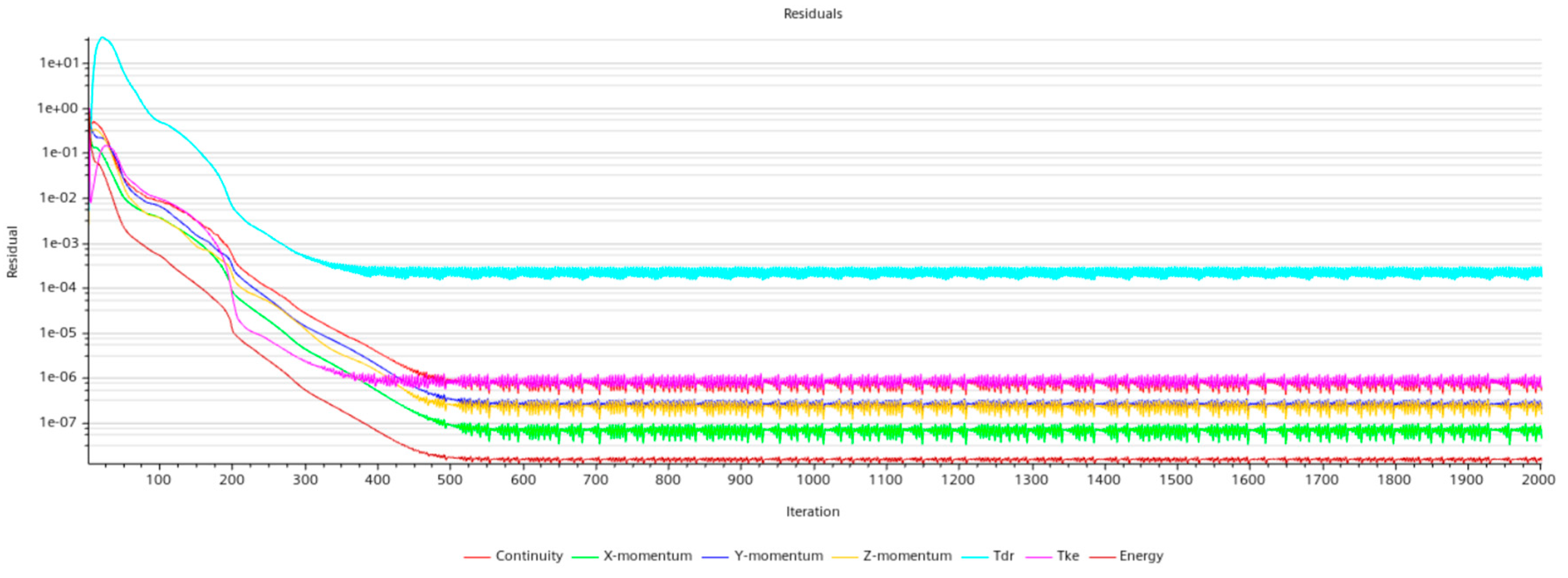
Figure 5: Residual histories of all governing equations during CFD simulation.

As illustrated, all the residuals decreased by several orders of magnitude over the course of the iterations. Specifically, the residuals of momentum and turbulence-related equations fell below 10 − 5 , and the continuity residual decreased to the order of 10 − 4 , which was taken as the threshold for acceptable convergence. Furthermore, the drag coefficient C d variation was monitored and observed to stabilize within less than 0.1% over the final 200 iterations, further confirming convergence of the solution.

Each simulation case was conducted on a workstation equipped with an Intel Xeon Gold 6226R (16 cores, 2.9 GHz) CPU and 64 GB of RAM. On average, each case required approximately 4.5 h of computation time and approximately 2000 iterations to reach convergence. This setup offers a practical balance between computational efficiency and result accuracy and is especially suitable for parametric optimization studies.

4 Research Results and Conclusions

Fig. 6 shows the four common angles of a vehicle. The angle of the engine hood α refers to the angle between the fixed top of the engine hood and the horizontal plane. The angle of the windshield β refers to the angle between the fixed lower edge of the windshield and the horizontal plane. The angle of the rear window γ refers to the angle between the fixed top edge of the rear window and the horizontal plane. The rear upwards tail lift angle θ refers to the angle between the fixed bottom of the rear and the horizontal plane.

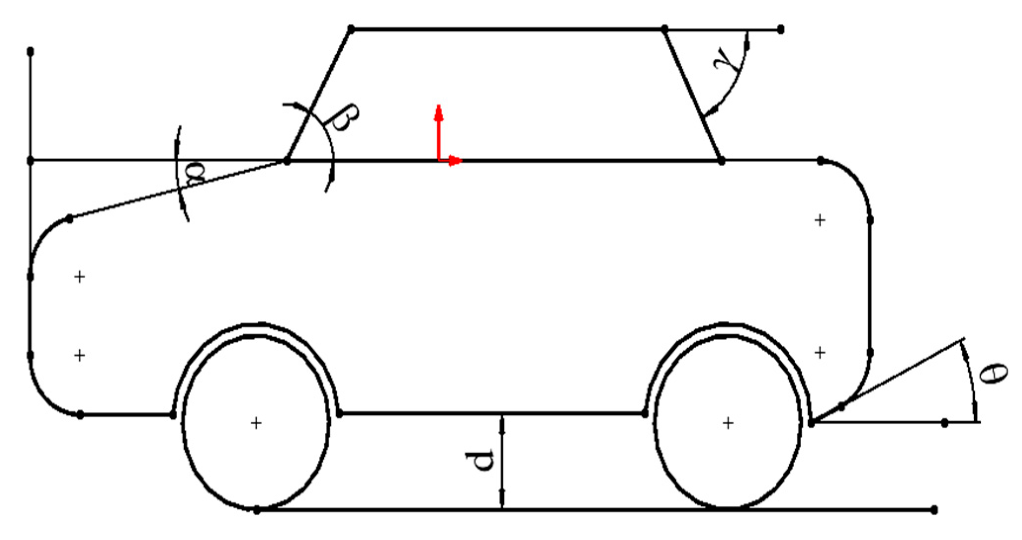
Figure 6: 2D parametric sketch.

This study is divided into three main parts: the front section of the vehicle, as shown in Fig. 7, which includes the engine hood angle α and the windshield angle β; the rear section, which includes the rear window angle γ and the upwards angle of the rear upwards tail lift angle θ; and the middle section, which includes the ground clearance d and the tilt angles.

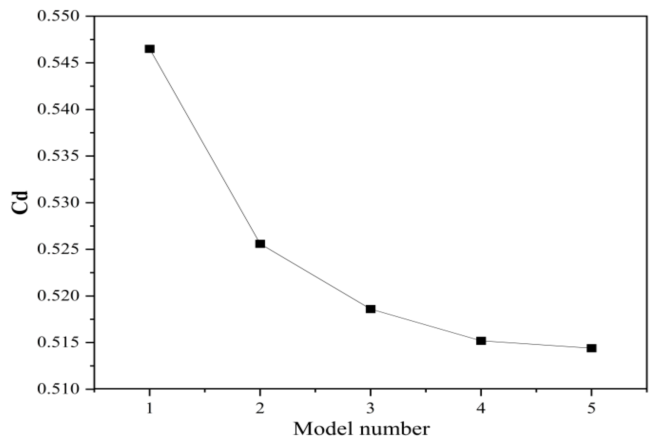
Figure 7: 3D parametric sketch.

In the course of conducting three-dimensional simulations, we reviewed a significant amount of literature and reported that numerical simulation results obtained using STAR-CCM+ often lack clarity. To improve the readability of the results and facilitate observation, we focused on the symmetry plane through the middle of the vehicle. This approach yielded clearer results, aiding the reader in better understanding and analysing the findings.

To gain further insight into the airflow behaviour around the vehicle, velocity vector contours were plotted along the central longitudinal plane for the configuration with a hood angle (α) of 5°, a windshield angle (β) of 25°, and a rear window angle (γ) of 50°, as shown in Fig. 8.

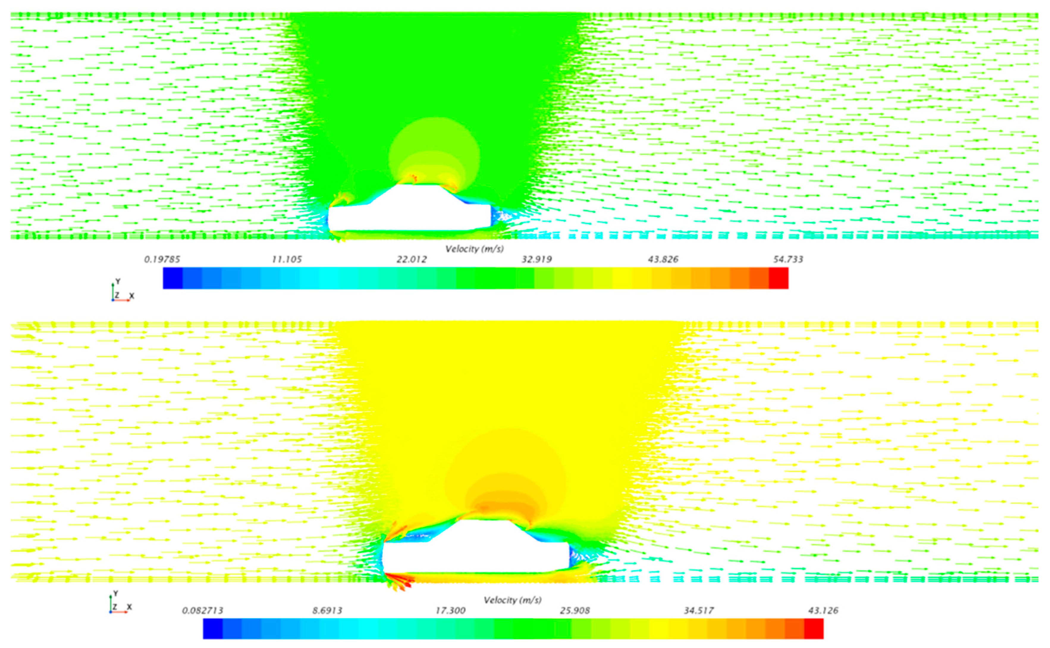
Figure 8: Velocity vector contours in the X-Z symmetry plane for the configuration α = 5°, β = 25°, γ = 50°.

The velocity vectors indicate smooth attached flow over the front hood and windshield area, with minimal separation. However, noticeable flow separation and wake formation are observed behind the rear window and upper roof edge, forming a distinct recirculation zone. The rear vortex structures are characterized by a sharp velocity drop and reversed flow near the wake centre, which contributes significantly to aerodynamic drag.

This visualization highlights the complex interaction between surface angles and external flow, and supports the conclusion that rear surface design plays a dominant role in vortex shedding and energy loss in bluff-body vehicle aerodynamics.

4.1 Front of the Car Body

The aerodynamic performance of a vehicle has an important effect on the energy efficiency and driving stability of new energy vehicles, and the angle of the engine hood and front windshield at the front of the vehicle play crucial roles.

The influence mechanism of the engine hood inclination angle (α) is mainly reflected in the following: 1. Owing to the smoothness of the air flow, a larger engine hood inclination angle can make the air flow more smoothly through the front of the vehicle, reducing the pressure in front. 2. When the air separation phenomenon is reduced, a larger inclination angle helps reduce the separation of air flow, allowing the air to flow more closely along the vehicle body surface and reducing air resistance.

The main influences of the front windshield inclination angle (β) are as follows: 1. Affecting the direction and distribution of the airflow, a larger front windshield inclination angle makes the airflow more likely to attach to the upper part of the vehicle body, reducing separation and vortex formation. 2. This affects the smoothness of air flow: a larger inclination angle allows the air to flow more smoothly over the roof, reducing the turbulent area on the top and rear of the vehicle.

Fig. 9 shows the pressure distribution at the front of the car under different engine hood tilt angles. As the engine hood tilt angle increases, the negative pressure area at the leading edge of the engine hood gradually decreases, reducing the area of aerodynamic drag. The airflow becomes smoother along the rear of the hood, separation phenomena diminish, and the airflow speed increases. Although the “dead water area” does not show a significant change in size, the high pressure within this area decreases, indicating more stable flow within the boundary layer as the hood tilt angle increases. These findings provide important insights for optimizing vehicle aerodynamic design and reducing aerodynamic drag, offering key information for understanding the impact of different design parameters on aerodynamic performance.

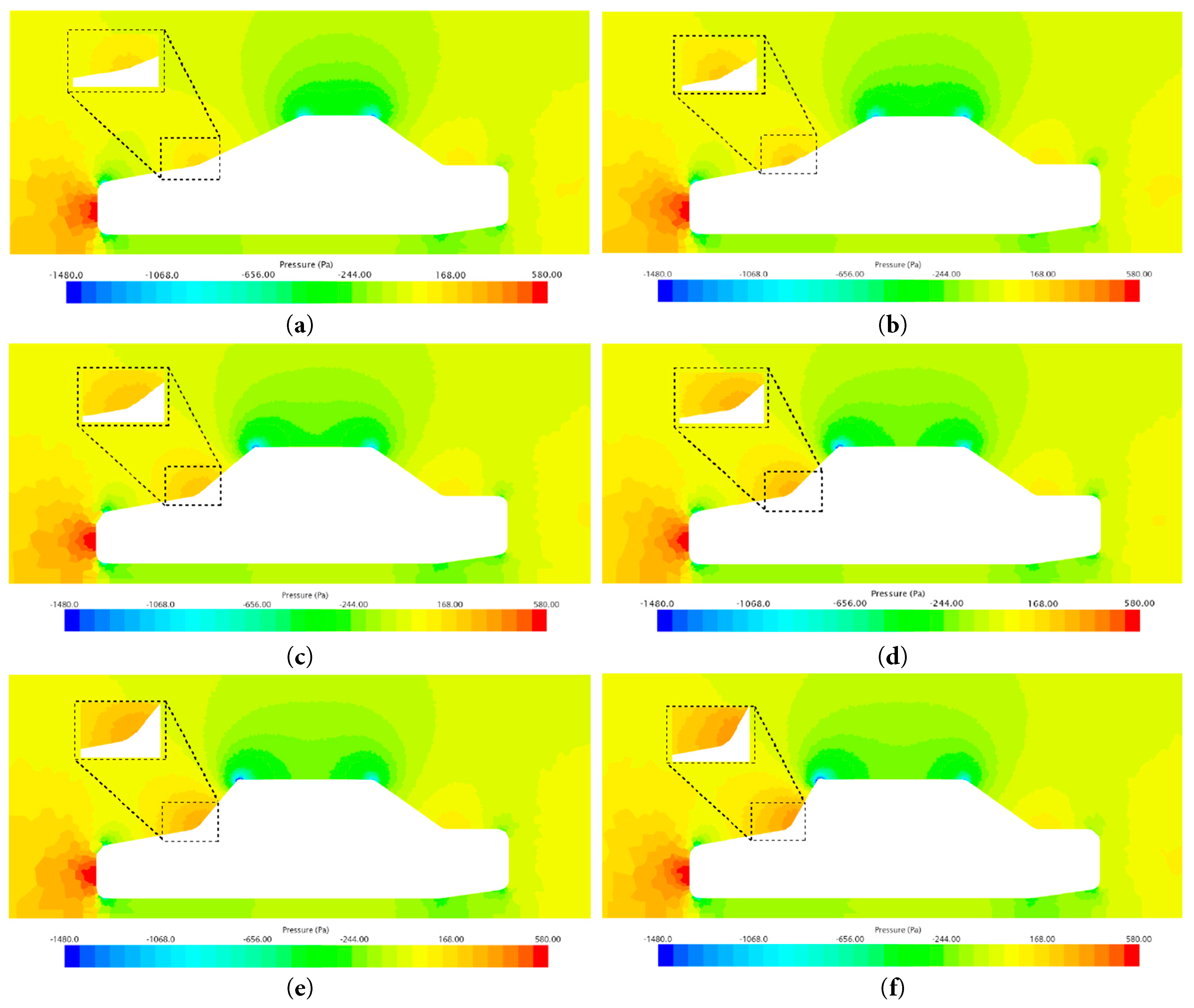
Figure 9: Pressure distribution diagram of different dip angles for α: (a) 0°; (b) 5°; (c) 7.5°; (d) 10°; (e) 15°; (f) 20°.

Fig. 10 shows the pressure distributions at the front of the car under different windshield tilt angles. As the windshield tilt angle increases, the following key phenomena are observed: airflow moves backwards along the hood and, upon encountering the windshield, creates a flow separation zone at the leading edge of the wind shield, known as the “dead water area” in aerodynamics. As the windshield tilt angle increases, the size of this “dead water area” gradually increases, leading to an increase in the front-end pressure, which in turn increases the drag coefficient value. Moreover, theoretically, the drag coefficient also significantly changes. From an aerodynamic perspective, a smaller windshield tilt angle is more favourable for reducing aerodynamic drag, but an excessively small angle may impair the driver’s visibility, affecting driving performance and safety. Therefore, in actual vehicle body design, it is essential to balance aerodynamic properties with driving performance requirements to find the optimal windshield tilt angle. These findings provide significant guidance and a deeper understanding for optimizing vehicle aerodynamic design.

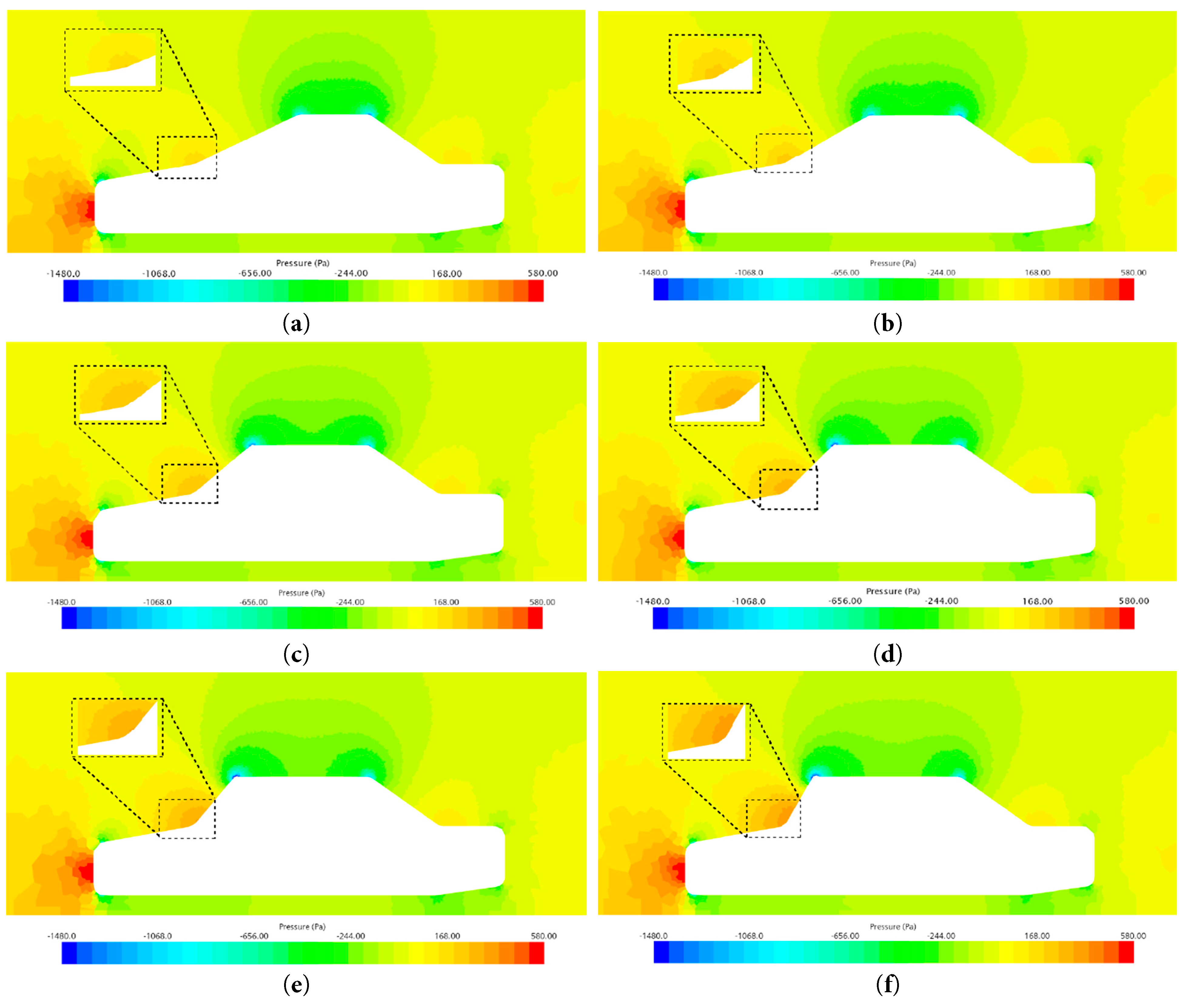
Figure 10: Pressure distribution diagram of different dip angles for β: (a) 25°; (b) 30°; (c) 40°; (d) 45°; (e) 50°; (f) 60°.

Fig. 11 shows that as the engine inclination angle α increases, the aerodynamic drag coefficient C d decreases, and as the front windshield inclination angle β increases, the aerodynamic drag coefficient increases. However, when the inclination angle is ≤30°, the aerodynamic drag coefficient C d does not change significantly. Overall, the minimum value of C d appears at α = 15° and β = 25°. In traditional vehicle design, the engine is usually located at the front of the vehicle. Therefore, when designing the engine hood inclination angle, the size of the engine must be considered, and a larger engine hood inclination angle may affect the engine layout. However, electric vehicles do not have an engine, so the engine hood inclination angle can be freely designed without affecting the aesthetic appearance to reduce air resistance.

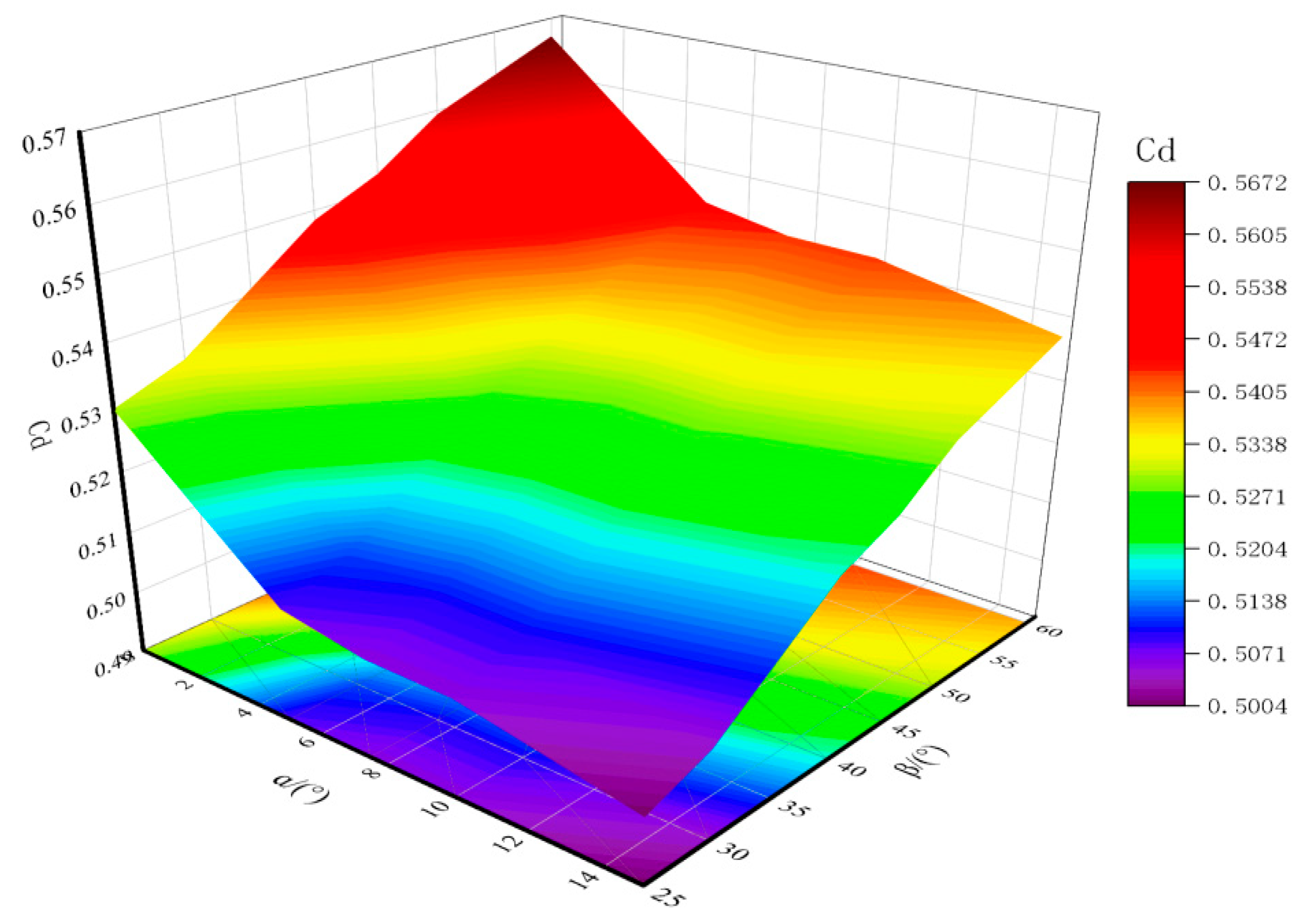
Figure 11: Aerodynamic drag coefficient C d  for different α and β.

4.2 The Rear of the Car Body

Fig. 12 shows the pressure distribution at the front of the car, primarily focusing on the positive pressure areas, especially in the middle and lower positions, with a maximum value of approximately 580 Pa. When the air flows over the roof, part of it continues along the direction of the windshield, whereas the other part flows horizontally along the roof, creating a negative pressure area at the junction of the rear window and the roof. Since the tilt angle of the rear window is smaller than that of the windshield, the pressure at the rear of the car is slightly lower than that at the front, making the airflow smoother, although the flow pattern is not very distinct. Additionally, in the area where the rear window intersects the roof, the pressure map shows a stepped pressure distribution: the sharper the angle is, the higher the pressure; the flatter the angle is, the pressure gradually decreases. These observations reveal the pressure distribution characteristics of different parts of the vehicle body and how these characteristics affect the vehicle’s aerodynamic performance and air resistance.

Figure 12: Pressure distribution diagram of different dip angles for γ: (a) 40°; (b) 50°; (c) 60°; (d) 70°.

Since the angle of the rear windshield in the upper part of the vehicle body is smaller than the angle of the front windshield, the pressure value in the rear part of the vehicle body is smaller than that of the front windshield, and the air flow is smoother, but the flow is not very clear or obvious. Furthermore, at the intersection of the rear windshield and the roof, the pressure diagram shows stepped diffusion, and the sharper the angle is, the greater the pressure; the more gradual the transition is, the gradually smaller the pressure.

Fig. 13 shows the changes in pressure at different angles: at 0°, the minimum pressure is −1414 Pa, the maximum pressure is 587 Pa, and the pressure difference is 1992 Pa; at 5°, the minimum pressure is −1408.2 Pa, the maximum pressure is 576.83 Pa, and the pressure difference is 1985.03 Pa; at 10°, the minimum pressure is −1252.8 Pa, the maximum pressure is 578 Pa, and the pressure difference is 1830.8 Pa; at 15°, the minimum pressure is −1259.9 Pa, the maximum pressure is 578.28 Pa, and the pressure difference is 1838.18 Pa; at 20°, the minimum pressure is −578.79 Pa, the maximum pressure is 1267.6 Pa, and the pressure difference is 1846.39 Pa. Therefore, when the departure angle is 10°, the pressure difference of the vehicle is the smallest, and the aerodynamic performance is the best.

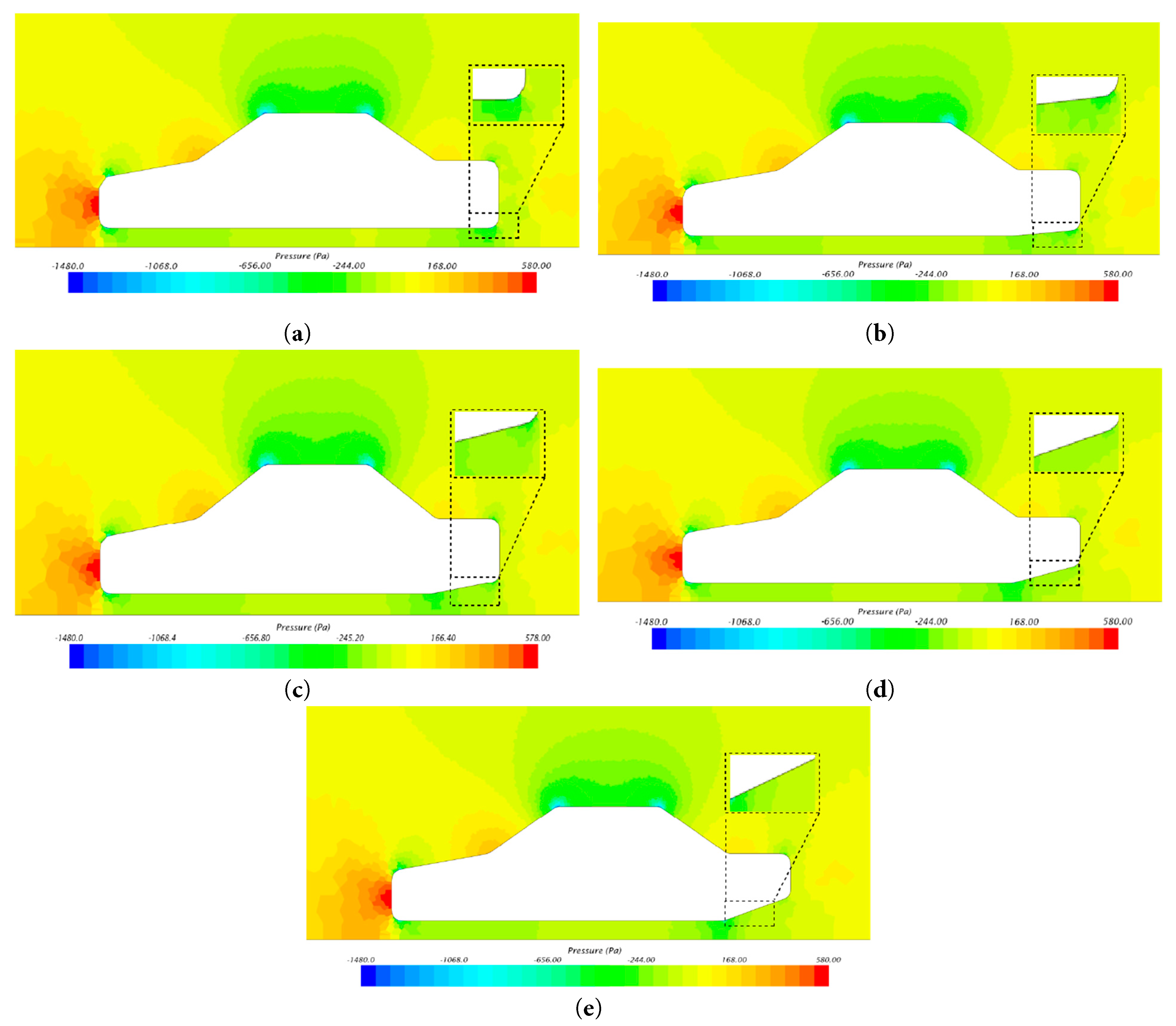
Figure 13: Pressure distribution diagram under different dip angles for θ: (a) 0°; (b) 5°; (c) 10°; (d) 15°; (e) 20°.

Fig. 14 shows the curve of the change in the air drag coefficient (Cd) with the change in the rear upwards tail lift angle (θ). When θ is relatively small, Cd increases and then decreases with increasing θ. When θ is 10°, Cd reaches the lowest value of 0.5176 and then gradually increases with increasing θ. As the rear windshield angle γ increases, the aerodynamic drag coefficient Cd increases significantly. When γ is greater than 50°, Cd decreases with increasing γ. When γ is 40°, Cd has a minimum value of 0.52. Overall, when θ is 10° and γ is 40°, the Cd value is the smallest.

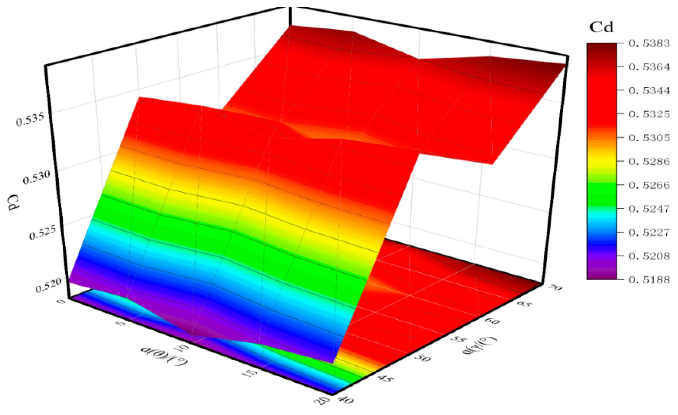
Figure 14: Aerodynamic drag coefficient C d  for different γ and θ.

4.3 The Middle Region of the Car Body

The optimization of the middle part of the vehicle body mainly focuses on the consideration of the vehicle’s ground clearance d and the side angle s of the vehicle body, as shown in Fig. 15:

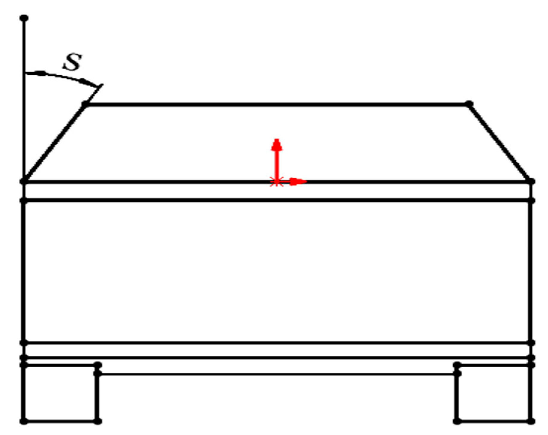
Figure 15: Car side angle.

The influence mechanism of the vehicle’s ground clearance on the resistance mainly involves the following aspects. First, the management of the bottom airflow directly affects the airflow path at the bottom of the vehicle. When the ground clearance is relatively low, the bottom airflow channel is narrower, the airflow is smoother, and there is less turbulence, thereby reducing the air resistance coefficient ( C d ). However, if the ground clearance is too low, the bottom airflow may be obstructed, resulting in a large pressure difference and an increase in the resistance coefficient. For the underbody pressure, a lower ground clearance usually increases the underbody pressure, improving the stability during high-speed driving. This is because as the bottom airflow velocity increases, the pressure decreases, and according to Bernoulli’s principle, a greater downwards force is generated. In this case, although an increase in the downwards force may increase the stability, it may also increase the air resistance.

Fig. 16 shows the pressure distributions under different front ground clearances. At 50 mm, the minimum pressure is −1430.0 Pa, the maximum pressure is 574.23 Pa, and the pressure difference is 2004.33 Pa. At 100 mm, the minimum pressure is −1418.3 Pa, the maximum pressure is 578.11 Pa, and the pressure difference is 1996.41 Pa. At 150 mm, the minimum pressure is −1438.5 Pa, the maximum pressure is 572.70 Pa, and the pressure difference is 2011.2 Pa. At 250 mm, the minimum pressure is −1250.5 Pa, the maximum pressure is 577.34 Pa, and the pressure difference is 1827.84 Pa. At 300 mm, the minimum pressure is −1408.9 Pa, the maximum pressure is 557.23 Pa, and the pressure difference is 1966.13 Pa. When the ground clearance is 250 mm, the pressure difference of the vehicle is the smallest, and the aerodynamic performance is the best.

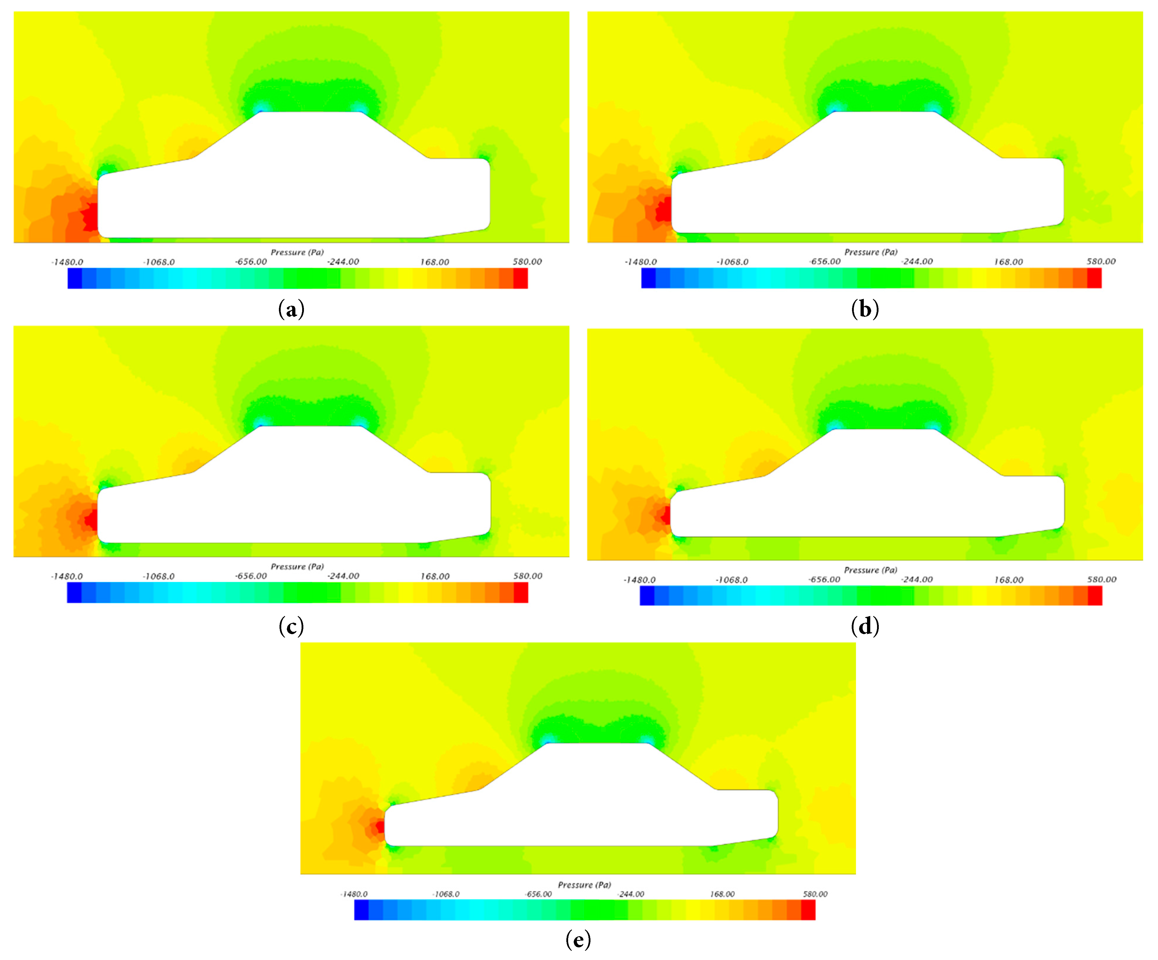
Figure 16: Pressure distribution diagram of different heights for d: (a) 50 mm; (b) 100 mm; (c) 150 mm; (d) 250 mm; (e) 300 mm.

Fig. 17 shows the pressure distributions at different angles. At 5°C, the minimum pressure is −345.53 Pa, the maximum pressure is −21.021 Pa, and the pressure difference is 324.50 Pa. At 10°C, the minimum pressure is −351.72 Pa, the maximum pressure is −20.464 Pa, and the pressure difference is 331.256 Pa. At 15°, the minimum pressure is −349.47 Pa, the maximum pressure is −20.575 Pa, and the pressure difference is 328.89 Pa. At 20°C, the minimum pressure is −351.37 Pa, the maximum pressure is −20.155 Pa, and the pressure difference is 331.155 Pa. When s is 5 degrees, the pressure difference of the vehicle is the smallest, and the aerodynamic performance is the best.

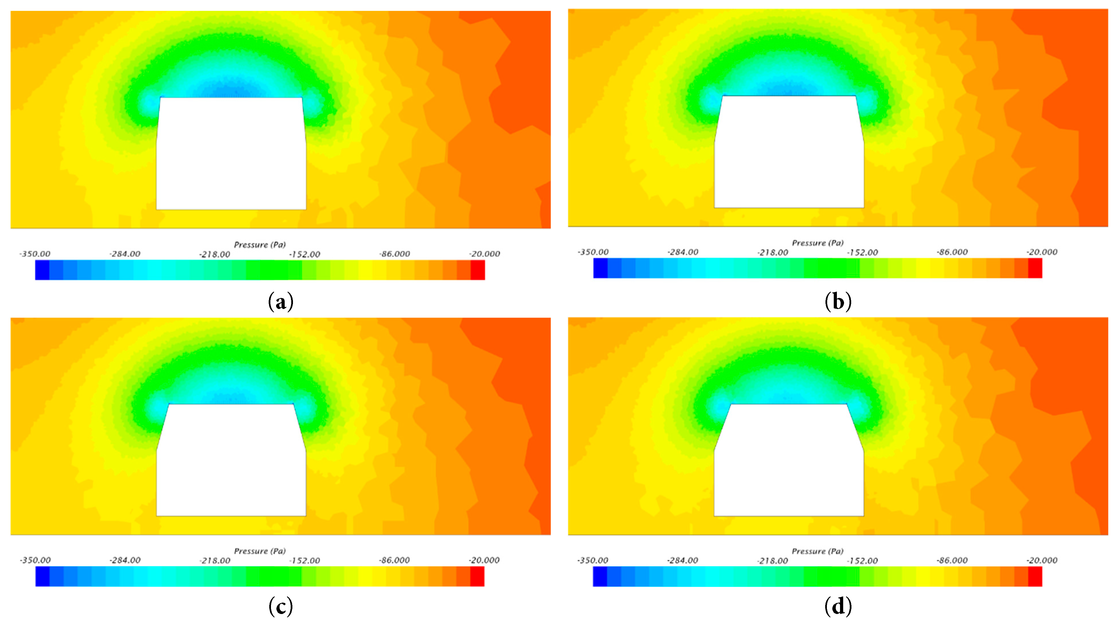
Figure 17: Pressure distribution diagram of different angles for s: (a) 5°; (b) 10°; (c) 15°; (d) 20°.

Fig. 18 shows that as the tilt angle increases, the air resistance coefficient also increases. As the ground clearance d increases, the air resistance coefficient C d reaches a minimum at 100 mm. When s is 5° and the ground clearance is 100 mm, the wind resistance is the lowest.

Figure 18: Aerodynamic drag coefficient C d  for different d and s.

5 Conclusion

This paper takes a new energy sedan as the research object and, through flow field simulation, summarizes the influence rules between the structural improvement of the vehicle body and the overall aerodynamic characteristics, which has certain research significance for the optimization of the vehicle body structure and the reduction in air resistance.

In this optimization study of the aerodynamics of new energy vehicles:

• 1.For the front part design, the optimized combination of an engine hood tilt angle (α) of 15° and a windshield tilt angle (β) of 25° reduces the air resistance coefficient (Cd). A reasonable angle design can effectively reduce the area of the aerodynamic “dead water zone”.
• 2.For the rear part design, as the rear windshield angle γ increases, the aerodynamic drag coefficient Cd increases significantly. When γ is greater than 50°, Cd decreases with increasing γ. The overall fluctuation range of the drag coefficient is not large with increasing rear spoiler angle (θ). The minimum value is obtained when (θ) is 10°. The theoretical air resistance coefficient (Cd) is minimized when the rear windshield angle (γ) is 40° and the rear spoiler angle (θ) is 10°.
• 3.For the middle part design, as the ground clearance gradually increases, the aerodynamic drag coefficient shows an overall increasing trend. Similarly, as the side angles of the vehicle body increase, the aerodynamic drag coefficient shows an overall upwards trend. A comprehensive consideration and overall optimization show that when the vehicle ground clearance (d) is set to 100 mm and the side angle (s) of the vehicle body is 5°, it meets the vehicle design, and the Cd value is within the ideal range.

The innovations of this paper mainly include the following: 1. The numerical simulation method can greatly shorten the R&D cycle and save costs, thereby improving the design efficiency. 2. The method of control variables is used to obtain the air resistance coefficient ( C d ) corresponding to different angles, thereby obtaining valuable data. 3. This study explores the impact of design variations in two key areas—the surface morphology of the vehicle body and the underbody—on a vehicle’s aerodynamic performance. Through numerical simulations and analysis, this research provides valuable insights into how these design changes affect a vehicle’s drag coefficient, stability, and overall aerodynamic efficiency.

This study is based on steady-state CFD simulations under idealized conditions, assuming uniform inlet flow aligned with the vehicle’s longitudinal axis and neglecting transient effects such as gusts or side winds. The tires were considered stationary, and ground motion was not simulated with a moving road or rotating wheels, which could influence underbody flow characteristics. Furthermore, all the simulations were carried out in a virtual wind tunnel using the standard k-ε turbulence model, which, while computationally efficient, may have limitations in accurately capturing complex separation and vortex dynamics.

To validate and complement these findings, future work should incorporate wind tunnel experiments or on-road testing under realistic operating conditions. Yaw angle-dependent studies (crosswind analysis) and unsteady simulations could provide a more comprehensive understanding of aerodynamic behaviour. Additionally, using more advanced turbulence models (e.g., SST k-ω or DES) and incorporating rotating wheels and moving ground could improve the simulation fidelity. These steps enhance the applicability of the simulation results to real-world vehicle design and performance optimization.

References

1. Naidu SRM, Madhavan VM, Chinta S, Manikandan R, Premkumar A, Girimurugan R. Analysis of aerodynamic characteristics of car diffuser for dissimilar diffuser angles on Sedan’s using CFD. Mater Today Proc. 2023;92:240–8. doi:10.1016/j.matpr.2023.04.379. [Google Scholar] [CrossRef]
2. Guerrero A, Castilla R, Eid G. A numerical aerodynamic analysis on the effect of rear underbody diffusers on road cars. Appl Sci. 2022;12(8):3763. doi:10.3390/app12083763. [Google Scholar] [CrossRef]
3. Qin P, Ricci A, Blocken B. CFD simulation of aerodynamic forces on the DrivAer car model: impact of computational parameters. J Wind Eng Ind Aerodyn. 2024;248:105711. doi:10.1016/j.jweia.2024.105711. [Google Scholar] [CrossRef]
4. Rostamzadeh-Renani M, Baghoolizadeh M, Sajadi SM, Rostamzadeh-Renani R, Azarkhavarani NK, Salahshour S, et al. A multiobjective and CFD based optimization of roof-flap geometry and position for simultaneous drag and lift reduction. Propuls Power Res. 2024;13(1):26–45. doi:10.1016/j.jppr.2024.02.004. [Google Scholar] [CrossRef]
5. Le Good G, Resnick M, Boardman P, Clough B. An investigation of aerodynamic effects of body morphing for passenger cars in close-proximity. Fluids. 2021;6(2):64. doi:10.3390/fluids6020064. [Google Scholar] [CrossRef]
6. Vignesh S, Gangad VS, Jishnu V, Krishna A, Mukkamala YS. Windscreen angle and hood inclination optimization for drag reduction in cars. Procedia Manuf. 2019;30:685–92. doi:10.1016/j.promfg.2019.02.062. [Google Scholar] [CrossRef]
7. Song KS, Kang SO, Jun SO, Park HI, Kee JD, Kim KH, et al. Aerodynamic design optimization of rear body shapes of a sedan for drag reduction. Int J Automot Technol. 2012;13(6):905–14. doi:10.1007/s12239-012-0091-7. [Google Scholar] [CrossRef]
8. Huminic A, Huminic G. Aerodynamics of curved underbody diffusers using CFD. J Wind Eng Ind Aerodyn. 2020;205:104300. doi:10.1016/j.jweia.2020.104300. [Google Scholar] [CrossRef]
9. Widodo WA, Karohmah MN. CFD based investigations into optimization of diffuser angle on rear bus body. Appl Mech Mater. 2016;836:127–31. doi:10.4028/www.scientific.net/AMM.836.127. [Google Scholar] [CrossRef]
10. Bayındırlı C, Çelik M. The determination of effect of windshield ınclination angle on drag coefficient of a bus model by CFD method. Int J Automot Eng Technol. 2020;9(3):122–9. doi:10.18245/ijaet.723755. [Google Scholar] [CrossRef]
11. Chen Q, Elrefaie M, Dai A, Ahmed F. TripNet: learning large-scale high-fidelity 3D car aerodynamics with triplane networks. arXiv:2503.17400. 2025. [Google Scholar]
12. Valencia A, Lepin N. Effect of spoilers and diffusers on the aerodynamics of a sedan automobile. Int J Heat Technol. 2024;42(4):1164–72. doi:10.18280/ijht.420406. [Google Scholar] [CrossRef]
13. Buscariolo FF, Assi GR, Sherwin SJ. Computational study on an ahmed body equipped with simplified underbody diffuser. J Wind Eng Ind Aerodyn. 2021;209:104411. doi:10.1016/j.jweia.2020.104411. [Google Scholar] [CrossRef]
14. Abdellah E, Wang B. CFD analysis on effect of front windshield angle on aerodynamic drag. In: Proceedings of the IOP Conference Series: Materials Science and Engineering; 2017 Mar 16–17; Chemnitz, Germany. doi:10.1088/1757-899X/231/1/012173. [Google Scholar] [CrossRef]
15. Jessing C, Stoll D, Kuthada T, Wiedemann J. New horizons of vehicle aerodynamics. J Automob Eng. 2017;231(9):1190–202. doi:10.1177/0954407017703245. [Google Scholar] [CrossRef]
16. Ashgriz N, Mostaghimi J. An introduction to computational fluid dynamics. Fluid Flow Handb. 2002;1:1–49. [Google Scholar]
17. Ferziger JH, Perić M. Computational methods for fluid dynamics. Berlin/Heidelberg, Germany: Springer; 2002. doi:10.1007/978-3-642-56026-2. [Google Scholar] [CrossRef]
18. Katz J, Plotkin A. Low-speed aerodynamics. Cambridge, UK: Cambridge University Press; 2001. doi:10.1017/CBO9780511810329. [Google Scholar] [CrossRef]
19. Schuetz TC. Aerodynamics of road vehicles. Warrendale, PA, USA: SAE International; 2015. doi:10.4271/r-430. [Google Scholar] [CrossRef]
20. Igali D, Mukhmetov O, Zhao Y, Fok SC, Teh SL. Comparative analysis of turbulence models for automotive aerodynamic simulation and design. Int J Automot Technol. 2019;20(6):1145–52. doi:10.1007/s12239-019-0107-7. [Google Scholar] [CrossRef]
21. Refaey HA, Alharthi MA, Abdel-Aziz AA, Elattar HF, Almohammadi BA, Abdelrahman HE, et al. Fluid flow characteristics for four lattice settings in brick tunnel kiln: CFD simulations. Buildings. 2023;13(3):733. doi:10.3390/buildings13030733. [Google Scholar] [CrossRef]
22. Heft AI, Indinger T, Adams NA. Introduction of a new realistic generic car model for aerodynamic investigations. München, Germany: Technische Universität München; 2012. Report No.: 2012-01-0168. doi:10.4271/2012-01-0168. [Google Scholar] [CrossRef]
23. Torckler R, Majidiyan H, Enshaei H. CFD-based design of novel drag-reducing appendages for container ships. Appl Ocean Res. 2025;158:104605. doi:10.1016/j.apor.2025.104605. [Google Scholar] [CrossRef]
24. Ahmad NE, Abo-Serie E, Gaylard A. Mesh optimization for ground vehicle aerodynamics. CFD Lett. 2010;2(1):54–65. [Google Scholar]
Cite This Article
Copyright © 2025 The Author(s). Published by Tech Science Press.
This work is licensed under a Creative Commons Attribution 4.0 International License , which permits unrestricted use, distribution, and reproduction in any medium, provided the original work is properly cited.
Downloads
Citation Tools