Unsteady Flow Dynamics and Phase Transition Behavior of CO₂ in Fracturing Wellbores

1 Introduction

CO2 fracturing possesses low surface tension, high fluidity, rapid return and discharge, superior seam-making capability, minimal reservoir damage, and effective production enhancement [1], which is highly significant for the exploration and development of low-permeability oilfields. Nonetheless, the physical properties of CO2 are susceptible to variations in temperature and pressure, which influence the fracturing impact. Consequently, precise forecasting of the temperature and pressure within the wellbore during the CO2 fracturing process is crucial for formulating an effective CO2 fracturing construction strategy.

Currently, there exist two primary methodologies for calculating wellbore temperature and pressure: (1) independent calculations of wellbore temperature and pressure, where in the temperature field is derived from the Ramey model [2] or through finite-difference distribution iteration [3]; (2) a coupled approach that synthesizes the equations of energy conservation, mass conservation, and momentum conservation.

Previously, Ramey [2] derived an approximate analytical solution for the wellbore temperature distribution for the heat transfer between water-based fracturing fluids and formations during drilling and oil and gas extraction and derived formulas for the display of wellbore temperature with respect to well depth and time, laying the foundation for a proposed steady-state model for wellbore heat transfer. Arnold [4] and Alves et al. [5] combined the wellbore heat transfer with a set of steady flow control equations and successively proposed analytical equations for wellbore temperatures under circulation and injection circumstances. Hasan and Kabir [6] and Hasan et al. [7] enhanced and refined the unsteady heat transfer temperature function derived from Ramey’s model to develop a more comprehensive temperature field model that accounts for the flow within the drilled wellbore. Gu et al. [8] established a temperature field model for concentric twin-pipe steam injection wells, building upon Ramey’s steady-state model. They integrated this with a computational model for the thermophysical properties of saturated steam and employed an iterative method to analyze wellbore heat loss during the injection of hot steam in these wells. Lv [9] formulated the wellbore energy equation for CO2 fracturing utilizing the first law of thermodynamics and developed a 1D + 1D transient fully-coupled wellbore temperature field model for CO2 fracturing in shale gas horizontal wells. This model integrates the continuity equation, the momentum equation, and a physical model that encompasses one-dimensional axial non-isothermal flow and one-dimensional radial unsteady heat transfer. The model is discretized employing a fully implicit finite difference method, and the discretized equations are implemented and resolved using MATLAB. Xiao [10] established a temperature-pressure field coupling calculation model by analyzing heat transfer and pressure propagation in wellbores and formation fractures during the supercritical CO2 dry fracturing pumping process and implemented finite difference solving using MATLAB for this model. Wu et al. [11] developed a transient temperature and pressure model for supercritical CO2 fracturing wellbores, incorporating the influences of axial thermal conductivity, the Joule-Thomson effect, work from expansion and compression, and the distribution of heat generated by friction. The study simulated and analyzed the effects of injection temperature, construction displacement, drag reduction, and tubing dimensions on the temperature, pressure, and phase state of the wellbore. Yao et al. [12] developed a transient wellbore-formation heat transfer model considering the effect of the IDP. Heat transfer control units are formulated based on energy conservation, discretized using the finite difference method, and solved with the Gauss-Seidel to determine wellbore temperature.

At the beginning of the 21st century, Al-Adwani [13] commenced the precise application of the Span-Wagner equation [14] for calculating the thermodynamic properties of CO2 in wellbore flow scenarios, which was later utilized for determining CO2’s thermal and physical properties under diverse operating conditions. Yasunami et al. [15] posited that the natural convective heat transfer of fluid within the annulus substantially influences the heat exchange between the wellbore and the formation, and the natural convective heat transfer coefficient in the annulus was determined experimentally. Ruan et al. [16] conducted numerical simulations to calculate wellbore pressures and temperatures, highlighting that convective heat transfer in the annulus significantly influences CO2 heat transfer. They demonstrated that compressibility, heat exchange, and potential energy loss are the three factors contributing to changes in wellbore temperature. Li [17] analyzed the interrelated flow and heat transfer in a CO2 fractured wellbore implementing the Span-Wagner equation [14] of state and the Fenghour transport property model, integrating mass, momentum, and energy conservation equations. This study uniquely employed a two-way coupled solution to analyze the variations in temperature and pressure within the wellbore. Luo et al. [18] developed equations for wellbore temperature and pressure in their investigation of the CO2 fracturing temperature field. They integrated the K-D-R method with a CO2 physical property model to formulate a calculation model for the wellbore and fracture temperature field during CO2 fracturing, subsequently validating the model’s accuracy through the alignment of measured temperature and pressure data. Guo et al. [19] conducted coupled numerical calculations of a CO2 physical property model, a CO2 fracturing wellbore pressure drop model, and a heat transfer model, based on the interdependent effects of wellbore temperature and pressure changes on CO2 physical properties and analyzed the governing principles of supercritical CO2 fracturing wellbore flow and heat transfer. Li et al. [20] analyzed the basic physical properties of carbon dioxide under different temperatures and pressures, and the changes of wellbore temperature and pressure during carbon dioxide fracturing are studied based on the generalized heat conduction theory. The results show that the faster the injection rate of CO2 fracturing fluid at the wellhead, the lower the bottom hole temperature and the higher the bottom hole pressure. However, the higher the wellhead injection temperature, the higher the bottom hole temperature, and the lower the bottom hole pressure. Sang [21] formulated a coupled model for flow and heat transfer, addressing axial unsteady flow within the wellbore, radial unsteady heat transfer, and the variation of CO2’s physical parameters, employing fully implicit differential discretization equations, and resolved the model utilizing a computer through a double iteration method.

Current research examining the impacts of fluid, wellbore, and formation axial heat transfer has determined that wellbore axial convective heat transfer minimally influences the overall temperature variation within the wellbore. This paper integrates one-dimensional axial non-isothermal flow with one-dimensional radial unsteady heat transfer to create a two-dimensional temperature-pressure coupling model. It segments the wellbore radially into a single-layer grid and the stratum into a multi-layer fractional inhomogeneous grid, thereby enhancing computational efficiency significantly.

2 Carbon Dioxide Fracturing Wellbore Temperature and Pressure Prediction Modelling

2.1 Carbon Dioxide Physical Characteristics

During fracturing operations, CO2 fluid is injected into the wellbore at high pressure and low temperature (pressure 30~60 MPa, temperature −20~−5°C), resulting in CO2 predominantly existing in a liquid or supercritical condition after being pumped into the pipe. The thermophysical parameters of CO2 (e.g., temperature and pressure) vary significantly due to formation conditions and flow friction. These variations are closely linked to phase state changes, making the fluid prone to phase transitions. To examine the heat transmission properties of CO2 fluid in the wellbore, it is essential to delineate the thermodynamic state parameter, enthalpy, which is intricately linked to the phase change process. Enthalpy is frequently utilized to characterize the energy alterations of fluids in various states; for instance, the phase behavior, phase transitions, and associated energy changes of oil and gas mixes are intricately linked to enthalpy.

Fig. 1 illustrates the curves of CO2 enthalpy as a function of temperature and pressure derived from the Refprop database. Fig. 1a illustrates the isothermal curves of CO2 enthalpy versus pressure. The blue line represents the enthalpy change of liquid CO2 with respect to temperature and pressure, while the green line depicts the enthalpy change of gaseous CO2 under the same conditions. The intersection point indicates the enthalpy value of CO2 at the critical point (7.38 MPa, 31.4°C), where the phase transition from gaseous or liquid state to supercritical state occurs, resulting in an enthalpy change of zero. Examination of Fig. 1a reveals that the five curves at 40°C, 60°C, 80°C, 100°C, and 120°C exhibit a progressive decline with increasing pressure, but the enthalpy of CO2 experiences a sudden alteration in response to pressure variations at −20°C, 0°C, and 20°C. This sudden alteration represents the enthalpy of phase transition during the evaporation of liquid CO2 into a gaseous state or the liquefaction of a gaseous state into a liquid state. When the critical temperature of CO2 is beyond, its enthalpy increases with rising temperature and decreases with increasing pressure; nevertheless, above a specific pressure threshold, the enthalpy begins to rise again.

Figure 1: Variation of enthalpy of CO₂ with temperature and pressure.

When CO2 is injected in its liquid state, contingent upon the regulation of construction parameters and variations in the actual wellbore environment, two scenarios arise regarding the CO2 fluid: one is that CO2 remains in a liquid state throughout the flow process, with no phase transition occurring. The other is that CO2 is transformed from a liquid state to a supercritical state due to the application of temperature and pressure. When CO2 transitions from a liquid to a supercritical state, the enthalpy of phase transition is zero, indicating the absence of a combination of liquid and supercritical phases [22].

The temperature and pressure of each node in the well section during CO2 flow in the wellbore were investigated to reliably predict the location of CO2 fluid phase transition when construction parameters such as pumping pressure and displacement are changed under fracturing conditions. The phase distribution of CO2 fluid in the well section during the fracturing process can be acquired and subsequently adjusted to reflect actual fracturing circumstances, facilitating the analysis of the coupling mechanism of the interaction force between the fluid and the tubing column during CO2 fracturing.

Fig. 2 illustrates the physical model of the micrometric section of the wellbore, with the length of the micrometric section designated as dz. Under CO2 fracturing conditions, CO2 fluid is injected through the pipe, while a static annular fluid medium exists within the annulus of the oil casing. The CO2 is injected during the process, and heat transfer encompasses forced convective heat exchange occurring during the flow of the CO2 fluid, as well as heat transfer between the tubing wall, cement annulus, and the formation.

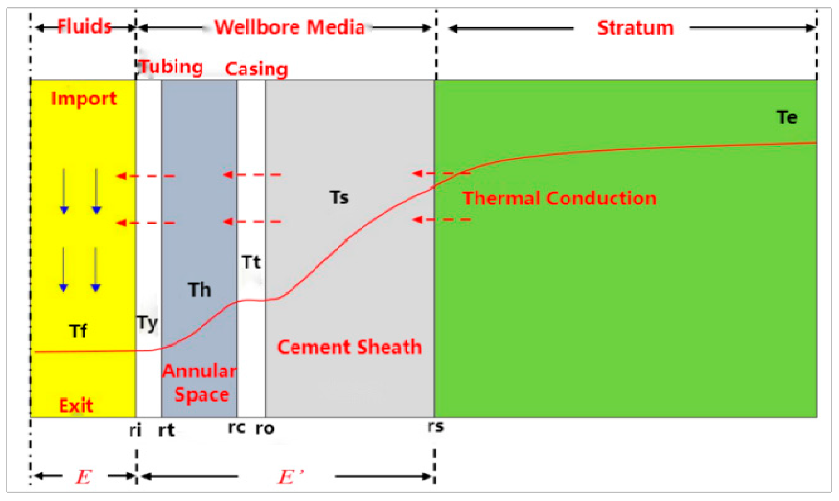
Figure 2: Microelementary physical model of CO₂ fractured wellbore.

According to the actual working conditions considering the complexity of CO2 fluid flow during CO2 fracturing, the following assumptions were made for the wellbore temperature and pressure model:

• (1)Physical parameters, including temperature, pressure, and flow velocity of CO2 at the identical cross-section, are maintained consistently;
• (2)Axial heat transfer in the wellbore is much less than radial and is thus negligible; (In the fully coupled model of CO2 fracturing wellbore flow, although the axial heat conduction terms should theoretically be considered, actual operational analysis shows that the Reynolds number under these conditions significantly exceeds 4000 (indicating turbulent flow). Theoretical studies by Tang et al. [23] demonstrate that the contribution axial heat conduction dominates in the low Reynolds number (Re < 4000) laminar flow regimes, while its influence becomes negligible in the high Reynolds number turbulent conditions. This conclusion aligns with the treatment of simplifying the axial heat conduction term in the CO2 fracturing numerical models established by Lv [9], Wu [11], and Guo et al. [19]. Therefore, in typical CO2 fracturing simulations, based on the thermodynamic characteristics of turbulent flow, the axial heat conduction term in the wellbore can reasonably be neglected without compromising model accuracy.);
• (3)Consistent operational parameters, including CO2 injection volume, injection temperature, and injection pressure;
• (4)The subsurface functions as a thermostatic zone, exhibiting a linear relationship between well depth and formation temperature once reaching a specific depth;
• (5)Pure CO2 fluid in the wellbore and CO2 gas in the annulus of the oil jacket.

2.2 Temperature-Pressure Coupled Calculation Model

The calculation area includes the CO2 area, the wellbore area and the formation area. The CO2 region exhibits non-isothermal flow and necessitates the simultaneous resolution of the continuity, momentum, and energy equations. The wellbore and formation regions involve natural convective heat transfer (annular) or solid heat transfer, necessitating the resolution of the energy equation.

2.2.1 Flow Simulation in Pipelines

The CO2 region continuity equation and momentum equation are shown in Eqs. (1) and (2), respectively: u∂ρf∂z+ρf∂u∂z+∂ρf∂t=0(1) ∂pf∂z=ρfgsinθ−12fDρfu2di−ρf∂u∂t(2) where ρf is CO2 density, with a value range of 900~1200 kg/m3, kg/m3; t is time, s; z is axial extension distance of wellbore, m; u is CO2 flow velocity, m/s; pf is CO2 pressure, Pa; di is inner diameter of tubing, m; fD is friction coefficient, which can be calculated by using the empirical formula of drag coefficient applicable to the full range of Reynolds number proposed by Chen [24].

In Eq. (3), e is the absolute roughness of the wall, with a value range of 1 × 10−5~5 × 10−5 m, m; dh is the hydraulic diameter, take the diameter of the oil pipe can be, m.

The Re number is calculated as:

In Eq. (4), μf is the CO2 kinetic viscosity, with a value range of 9 × 10−5~1.5 × 10−4 Pa·s, Pa·s.

Under CO2 fracturing conditions, the injection velocity of CO2 typically exceeds 3 m3/min, utilizing tubing with an inner diameter of 76 mm for injection. At a wellhead temperature of −20°C and a pressure of 25 MPa, the Reynolds number for CO2 in the tubing can reach 8.69 × 106, as calculated using Eq. (4), indicating that CO2 is in a turbulent condition throughout the fracturing process. Turbulent flow results in more vigorous fluid mixing, a reduced thermal boundary layer thickness, and enhanced heat transfer efficiency compared to laminar flow.

The energy equation for the CO2 region is shown in Eq. (5): Aρfcpf∂Tf∂t+u∂Tf∂z=Qw+Qf+Qp(5) where A is the cross-sectional area of the tubing, m2; cpf is the specific heat capacity of CO2, J/(kg·K); Tf is the temperature of the CO2 fluid, W/(m·K).

Qw is the heat flow generated by wall heat transfer per unit length in the axial direction, W/m, defined as:

In Eq. (6), Ty is the temperature of the oil pipe, K; hy is the coefficient of forced convection heat transfer on the wall of the oil pipe, W/(m2·K), which can be calculated by the following equation [25].

In Eq. (7), Pr is the CO2 Prandtl number, defined as [26]:

Qf is the heat flow from viscous dissipation per unit length in the axial direction, W/m, defined as [27]:

Qp is the heat flux produced by pressure work per unit length in the axial direction, W/m, defined as [9]:

In Eq. (10), αf is the coefficient of isobaric thermal expansion of CO2, 1/K, defined as:

2.2.2 Flow Boundary Modelling

The wellbore region includes the tubing wall, the annulus, the casing wall, and the cement ring. With the exception of the annulus, the remaining area is in a solid phase, necessitating consideration solely of heat transfer. The fluid within the annulus undergoes natural convection, characterized by the natural convection heat transfer coefficient. The elements of the wellbore region are categorized into a single-layer grid comprising the tubing wall, annulus, casing wall, and cement ring in the vertical portion (sloping section) and the tubing wall and annulus in the horizontal part. The equations governing the components of the wellbore are delineated individually for the vertical (sloping) and horizontal portions, taking into account the distinct boundary qualities among the various components of the wellbore region.

Fig. 3 illustrates the radial temperature and geometric mesh partition of the vertical section (slant-making section), and the equations for controlling the energy of the pipe wall, casing annular air, casing wall, and cement ring are as follows:

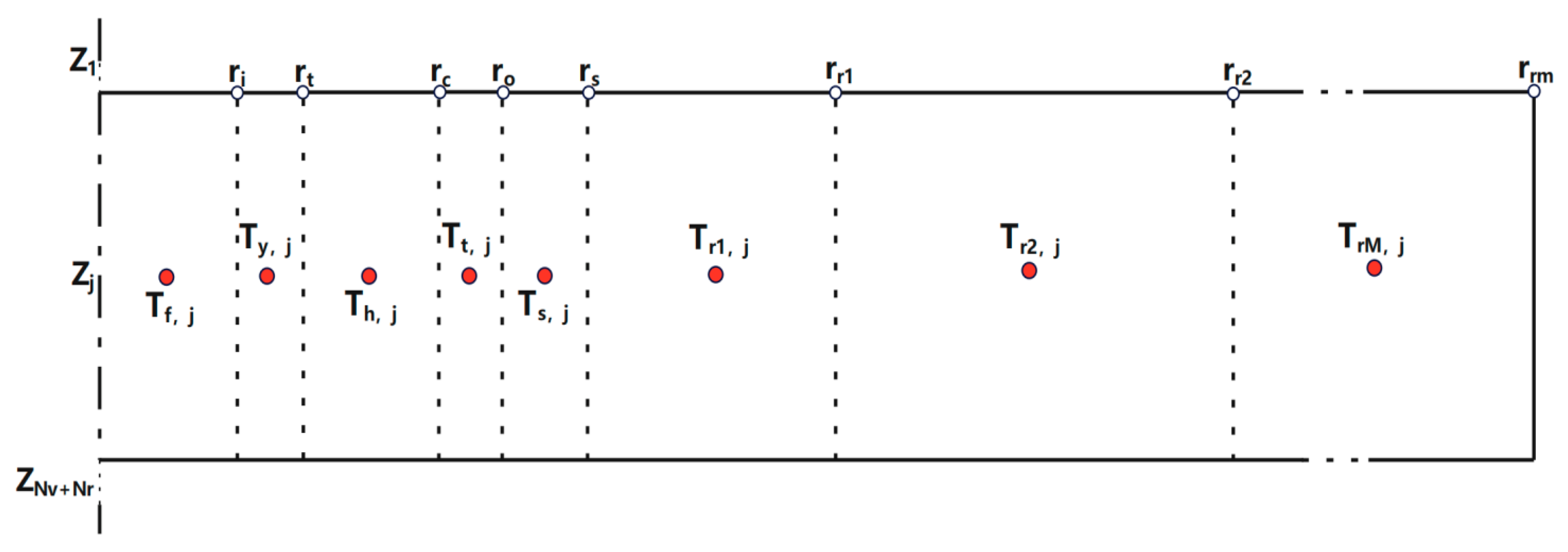
Figure 3: Radial meshing of vertical section (sloping section).

Energy control equations for oil pipe walls:

Energy control equations for the ring-space:

Energy control equations for casing wall:

Energy control equations for cement ring:

In Eqs. (12)–(15): rt is the outer radius of the tubing, m; Th is the temperature of the annulus, °C; Ty is the temperature of the tubing, °C; hh is the coefficient of natural convection heat transfer, W/(m2·K); rc is the inner radius of the casing, m; ρh is the density of the annulus, kg/m3; cph is the specific heat capacity of the annulus, J/(kg·°C); Tt is the temperature of the casing, °C; ro is the outer radius of the casing, m; ρt is the casing density, kg/m3; cpt is the casing specific heat capacity, J/(kg·°C); Ts is the cement ring temperature, °C; rs is the outer radius of the cement ring, m; ρs is the density of the cement ring, kg/m3; cps is the specific heat capacity of the cement ring, J/(kg·°C); λt,h and λs,r are the composite thermal conductivity.

Using Dropkin and Somerscales [28] equation for the equivalent heat transfer coefficient between flat plates to make an approximation to hh as follows:

In Eqs. (16)–(18): Grh is the Grashof number of the annular fluid; Prh is the Prandtl number of the annular fluid; λh is the thermal conductivity of the annular fluid, W/(m·°C); ρh is the density of the annular fluid, kg/m3; μh is the viscosity of the annular fluid, Pa·s; cph is the constant-pressure specific heat capacity of the annular fluid, J/(kg·°C); βh is the thermal expansion coefficient of the annular fluid, 1/°C.

λt,s and λs,r can be calculated from Fourier’s law:

The meshing of the horizontal segments is shown in Fig. 4.

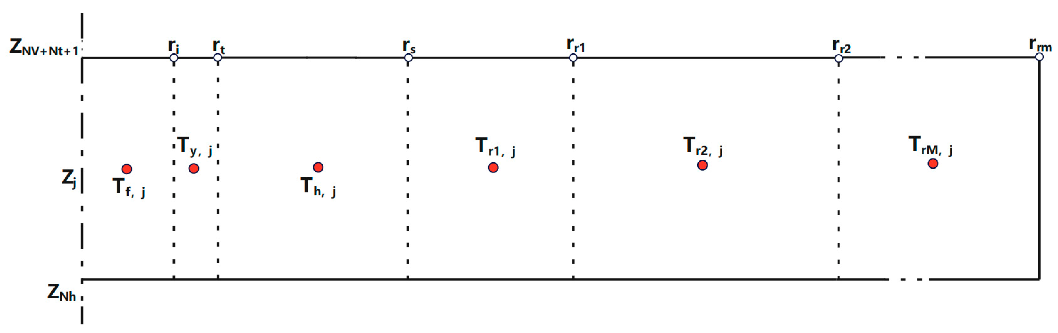
Figure 4: Schematic diagram of radial meshing of horizontal section.

The horizontal section of the wellbore consists only of the tubing wall and the annulus, where the energy control equations for the tubing wall are the same as those for the vertical section (inclined section), see Eq. (12). The energy control equation of the annulus is as follows:

2.2.3 Stratigraphic Regional Thermal Conductivity Modelling

There is no flow within the formation, so the energy control equation within the formation can be simplified to the heat transfer equation:

The divergence in radial grid configuration between the vertical (inclination-building) segment and the lateral section necessitates distinct equation formulations at the formation-wellbore boundary interface.

First stratigraphic grid of the vertical section (orographic section):

First stratigraphic grid of horizontal section:

In Eqs. (16)–(18): rri is the location of the ith grid of the stratum, m; Tri is the temperature of the ith grid of the stratum, °C.

2.3 Calculate Boundary and Initial Conditions

2.3.1 Initial Conditions

The initial wellbore temperature is derived from the original ground temperature gradient. The starting wellbore pressure, assuming the wellbore is filled with CO2, can be determined as the static liquid column pressure at the initial time by an iterative method integrated with the CO2 density model. The governing equations for the initial conditions are as follows: Tt=0=Tsurf+TD⋅zpt=0=∫0zρT,pgdz(25) where Tsurf is the surface temperature, °C; TD is the ground temperature gradient, °C/m.

2.3.2 Boundary Conditions

In the CO2 regional flow field, the injection displacement is specified at the wellhead as the velocity boundary, while the pressure must be provided at the well’s bottom. This paper utilizes the fracture closure pressure, defined as the minimum pressure necessary for fracture extension, as the pressure boundary at the well’s base. The injection temperature is specified at the wellhead as the temperature boundary for the CO2 regional temperature field, with adiabatic conditions at the bottom of the well while accounting for thermal convection. The governing equations for the boundary conditions are as follows: uz=0=Qinj/πrti2pz=zbh=pwTz=0=Tinj∂T∂zz=zbh=0(26) where Qinj is the injection displacement, m3/s; pw is the fracture closure pressure at the bottom of the well, Pa; Tinj is the injection temperature, °C; zbh is the depth of sounding at the bottom of the well, m.

For the radial heat transfer in the wellbore region formation region and the inner boundary adjacent to the CO2 region, the heat flow is determined by the temperature difference between the CO2 and the pipe wall; the temperature at the outer boundary of the formation is taken as the original formation temperature at a constant temperature, and the control equations are as follows:

This model uses a fixed bottom-hole pressure boundary (Eq. (26)), which is suitable for pressure control analysis during the fracture propagation stage but does not consider the feedback of reservoir seepage on phase change. If CO2 seeps through the reservoir matrix (such as low-permeability shale), its vaporization critical point may be controlled by the near-well pressure gradient, necessitating further introduction of Darcy’s law and phase equation coupling for solution.

2.3.3 Coupled Iterative Methods

The coupled solution of temperature and pressure within the wellbore can be approached by first dividing the wellbore into small N segments. Boundary conditions for temperature and pressure are set at the wellhead, and the temperature and pressure distribution values for the small segments at the wellhead are calculated. If the calculated results deviate significantly from the actual values, the parameters are adjusted and corrected, and the process is repeated until the desired accuracy is achieved. Subsequently, iterations are performed along the length of the wellbore. By repeating this process, we ultimately determine the distribution patterns of CO2 temperature and pressure within the wellbore throughout the entire fracturing operation. The final program design process and specific steps are as Fig. 5 follows:

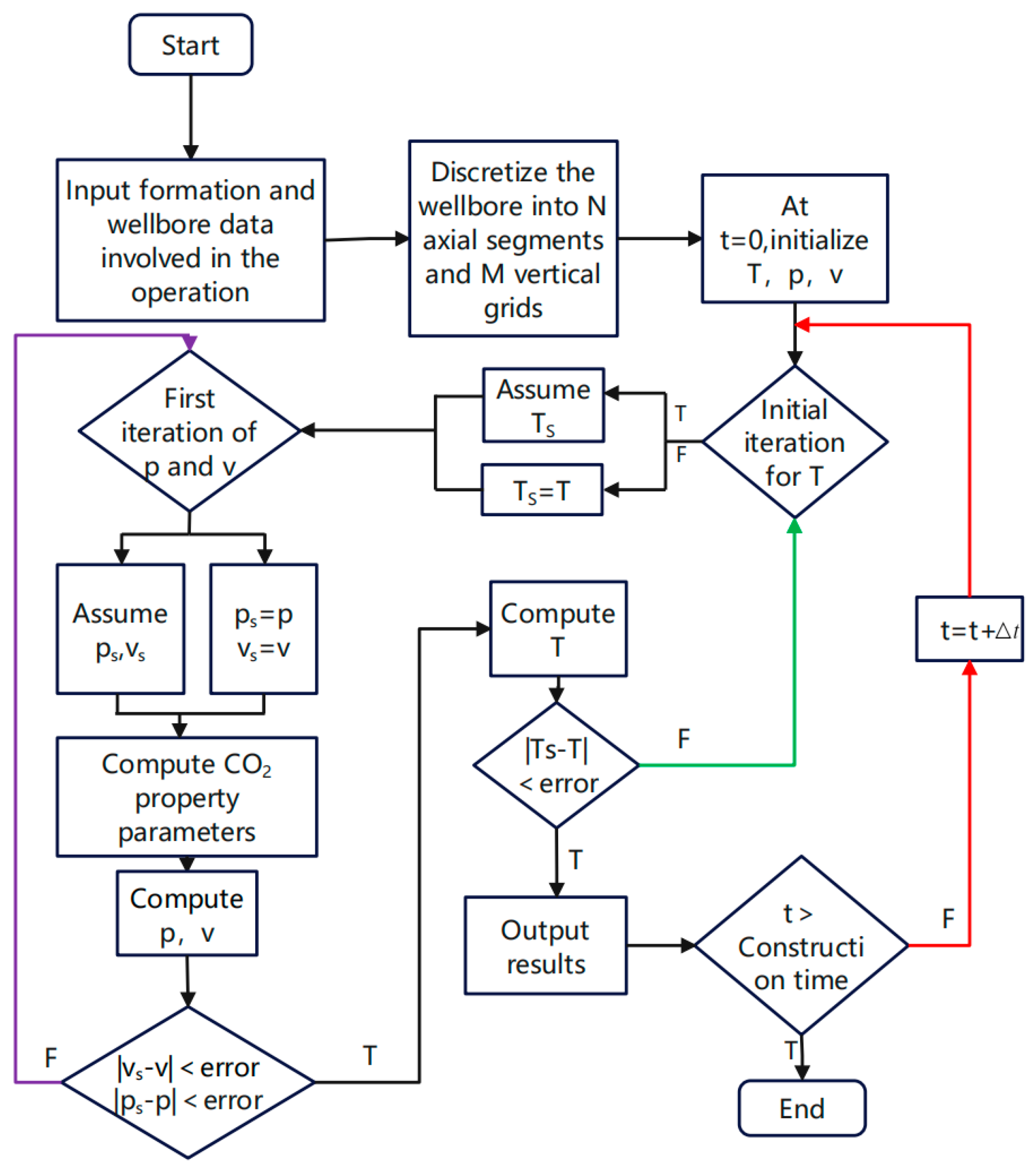
Figure 5: Program flowchart.

• (1)Divide the wellbore computational domain into spatial and temporal grids. The wellbore computational domain is divided into N elemental segments, with the upper endpoint of the elemental segment at the wellhead being Z0 and the lower endpoint of the elemental segment at the well bottom being ZN;
• (2)Input the base parameters of the wellbore, such as well depth, internal diameter, wall thickness, etc.;
• (3)Input the temperature and pressure at the wellhead Z0 are used to call Refprop for obtaining the physical properties of CO2, such as density, viscosity, thermal conductivity, enthalpy, etc., which provides the initial calculation data, and then substitute it into the model for solving;
• (4)Solve for the temperature increment ΔT0, pressure increment ΔP0, and enthalpy increment ΔH0 of the wellbore microelement section based on the discretized results of the constructed model;
• (5)Judge whether the ΔT0, ΔP0, ΔH0, calculated value is within the error allowable range. If not, return to step (4) to recalculate the temperature and pressure distribution in the wellbore micro-element section until the error allowable range is satisfied; if it meets the requirements, output the temperature and pressure values as well as the enthalpy value at the lower end point Z0+1 of the wellhead micro-element section;
• (6)After obtaining the temperature and pressure values and the enthalpy at the lower end point Z0+1 of the wellhead microelement section, Refprop was re-called to obtain the physical parameters of the CO2 fluid and to determine the phase of CO2;
• (7)The parameters at the lower end point Z0+1 of the 1st microelement section of the wellbore are the initial values of the 2nd microelement section, and the cycle of steps (3) to (6), and so on, iteratively solving until the temperature and pressure values at the lower end point ZN of the N-th micro-element section of the wellbore are obtained;
• (8)After the above solution steps, the temperature field and pressure field distribution within the entire wellbore are obtained; by processing the data accordingly, the distribution of the CO2 fluid phase state along the well depth under fracturing conditions can finally be obtained.

3 Carbon Dioxide Fracturing Wellbore Parameter Prediction Results

CO2 fracturing is performed using a horizontal well structure with a vertical section of 2000 m, an inclined section of 500 m and a horizontal section of 1500 m. P110 5-1/2″ casing with 7.72 mm wall thickness and N80 3-1/2″ tubing with 6.45 mm wall thickness. Wellhead fracturing fluid temperature: −20~−5°C, wellhead discharge: 2~5 m3/min, formation temperature gradient: 1.5~3.5°C/100 m. Fracturing construction Displacement is 2~10 m3/min, wellhead pressure is 15~35 MPa, and wellhead temperature is −12~−20°C.

3.1 Time-Domain Variation of Wellbore Parameters

Using an injection velocity of 2 m3/min, a wellhead temperature of −15°C, and a wellhead pressure of 50 MPa as construction parameters, the non-steady-state changes after CO2 fracturing injection were obtained. Fig. 6 shows the fluid flow process over a period of time after CO2 fracturing injection. After the low-temperature CO2 fracturing fluid is injected into the tubing, a radial temperature gradient of no more than 10 cm gradually forms in the annulus, casing and cement ring. When the fracturing fluid flows through the entire pipe section, a relatively stable radial temperature gradient is formed. The temperature gradient at the far end of the formation is the preset value, and it is less affected by the low-temperature medium in the wellbore.

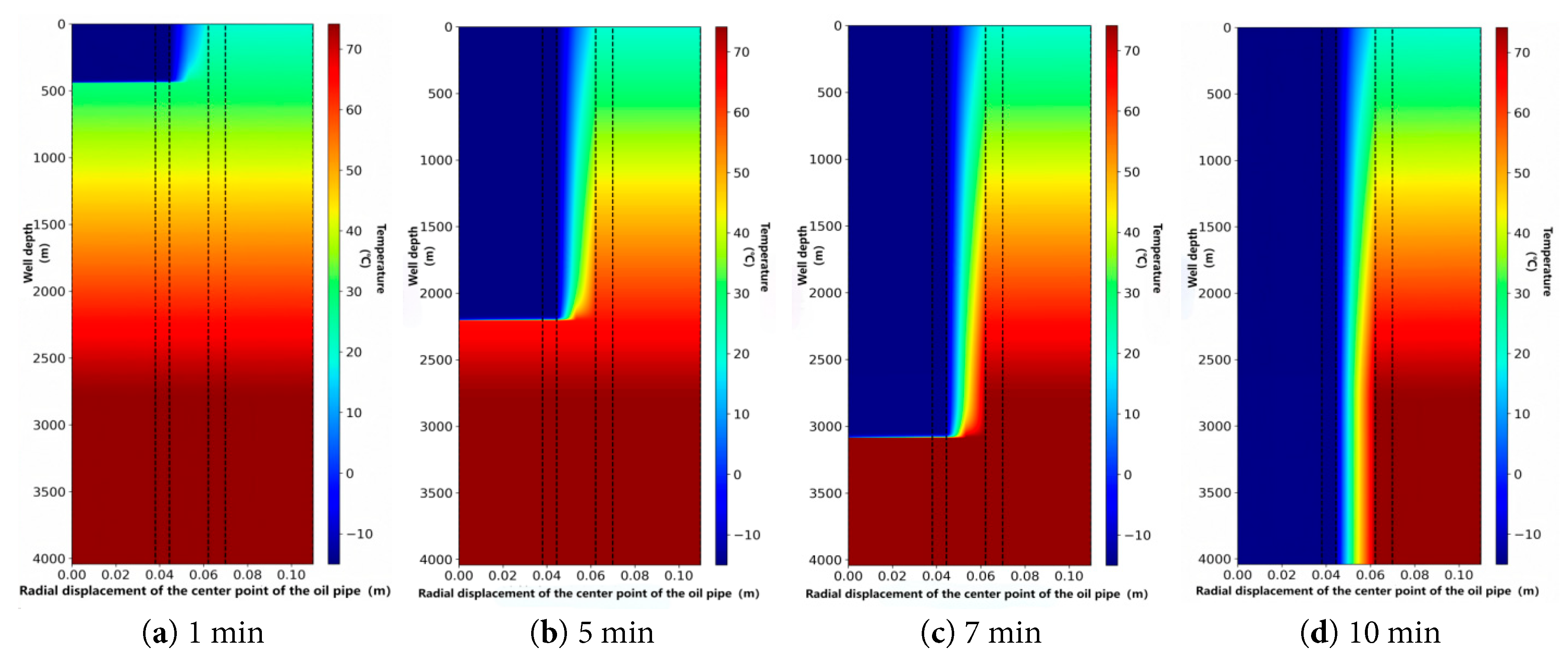
Figure 6: Temperature variation during CO₂ fluid injection into the wellbore.

After the CO2 fluid is injected into the wellbore, the flow velocity and other parameters of the CO2 fluid change due to the influence of the wellbore environment, as shown in Fig. 7. In the vertical section of the well, the temperature of the CO2 increases by approximately 5~10°C, and the pressure changes insignificantly, leading to volume expansion and a decrease in density. According to the continuity equation, a decrease in density will increase in velocity. In the horizontal section, The temperature of the cement ring tends to stabilize, and under high-temperature conditions, some liquid CO2 vaporizes, continuously absorbing heat and expanding, causing the pressure to sharply increase from 48 MPa to 68 MPa. Limited by the outlet area of the formation, the density increases within the confined space. According to the continuity equation, an increase in density will lead to a decrease in velocity.

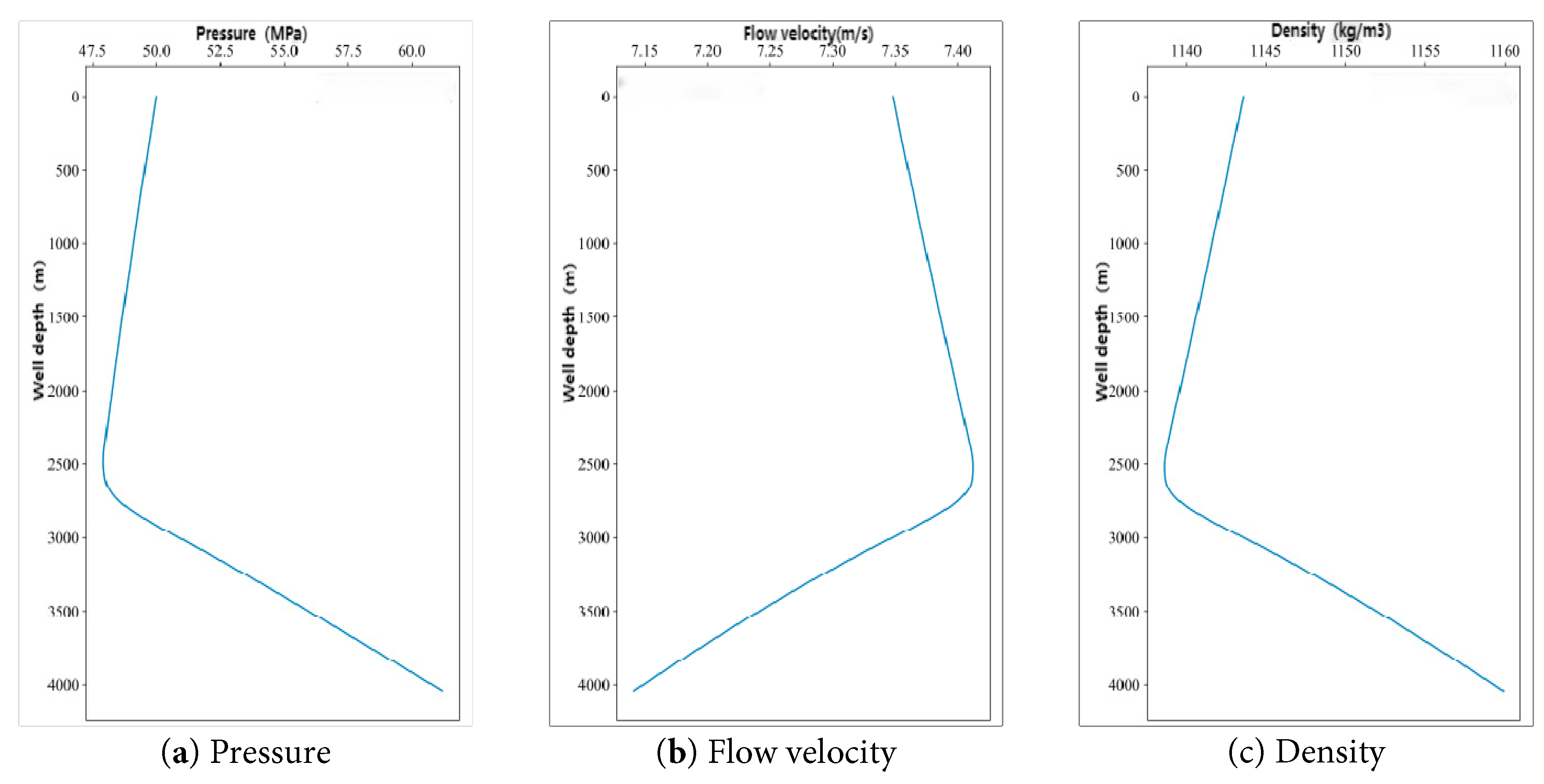
Figure 7: Variation of each parameter during CO₂ fluid injection into the wellbore.

3.2 Impact of Fracturing Construction Parameters

3.2.1 Injection Time Variation

By changing the injection time, the wellbore pressure and temperature are compared. Setting the displacement range 8 m3/min, wellhead temperature −15°C, wellhead pressure 20 MPa. The changes in temperature, pressure, flow velocity, and density parameters at different injection times are obtained, with the results shown in Fig. 8 and Fig. 9.

Fig. 8 shows the temperature variation curves of the casing, casing inner wall, and cement ring with well depth under different CO2 fracturing injection times. Temperature monitoring includes three positions: the casing inner medium, casing wall, and cement ring. The fracturing fluid reaches 4000 m from the wellhead to the bottom of the well, the temperature changes in the casing and casing wall are consistent with the initial formation temperature gradient, which decreases rapidly to the temperature of the fracturing fluid in the tubing, which is mainly affected by convection. The cement ring is not in direct contact with the medium inside the tubing and is affected by the radial thermal conductivity of the wall, which decreases by about 8°C in the wellhead section and 20°C in the horizontal section after 10 min.

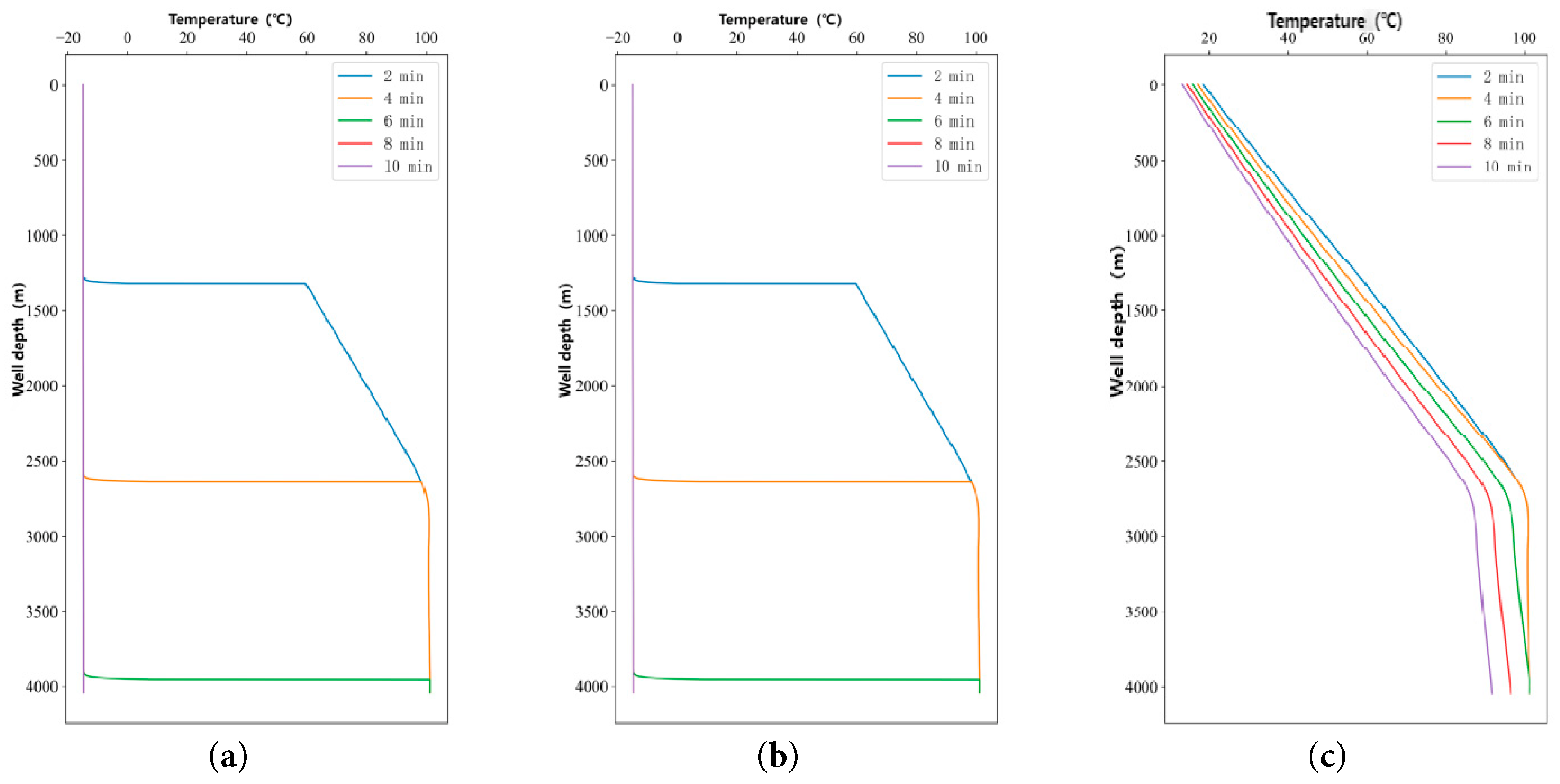
Figure 8: Variation of temperature in various parts of the wellbore with well depth. (a) Casing temperature; (b) Casing inner wall temperature; (c) Temperature of the cement sheath.

Fig. 9 shows the variation curves of CO2 fluid characteristics within the casing with depth under different injection times during CO2 fracturing. In the vertical section, the temperature of CO2 increases by approximately 8°C, leading to volume expansion and pressure increase. Changes in density and flow velocity are not significant. In the horizontal section, the cement ring temperature tends to stabilize, the CO2 continues to absorb heat and expand in the high-temperature environment, the pressure rises significantly, the density increases, and the flow velocity decreases.

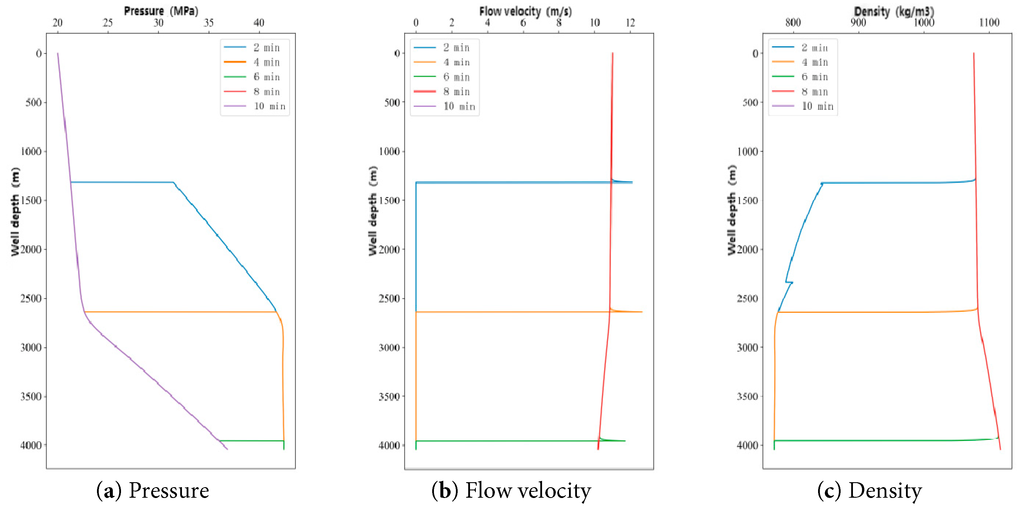
Figure 9: Variation curve of CO₂ fluid properties in casing with well depth.

3.2.2 Wellhead Temperature Changes

By changing the wellhead temperature, the wellbore pressure and temperature are compared. Setting wellhead temperature −20°C, −18°C, −16°C, −14°C, −12°C, fracturing displacement 8 m3/min, wellhead pressure 20 MPa. The changes of temperature, pressure, flow velocity, and density parameters under different wellhead temperatures were obtained, respectively, and the change results are shown in Fig. 10 and Fig. 11.

Fig. 10 shows the temperature variation curves of the casing, casing inner wall, and cement ring with well depth under different wellhead temperatures during CO2 fracturing. As the temperature of the fracturing fluid injected at the wellhead changes, the temperature within the casing and the casing wall does not vary significantly with well depth, and the temperature of the cement ring is consistent with the formation temperature. This is because it takes only 150 s to 160 s for liquid CO2 to flow from the wellhead to the bottom of the well. In such a short time, the temperature difference in the cement ring is very small, and the heat absorption of the liquid CO2 in the wellbore is also very small, so the temperature difference does not change significantly.

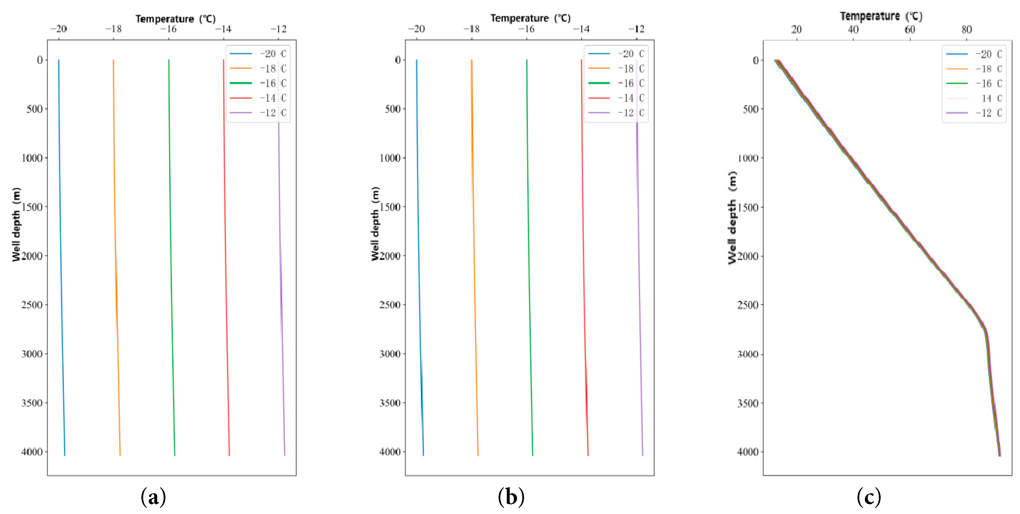
Figure 10: Variation of temperature in various parts of the wellbore with well depth. (a) Casing temperature; (b) Casing inner wall temperature; (c) Temperature of the cement sheath.

Fig. 11 shows the variation curves of CO2 fluid characteristics in the casing with depth under different wellhead temperatures during CO2 fracturing. With the temperature changes of the fracturing fluid injected at the wellhead in the vertical section, the pressure and flow velocity differences within the pipe are relatively small. In the horizontal section, under the high temperature of the formation, the vaporization of CO2 continues to absorb heat and expand, resulting in a significant increase in pressure, with relatively small changes in flow velocity. Density is affected by temperature, 1072 kg/m3 at wellhead temperature −14°C, bottom hole density 1110 kg/m3. 1094 kg/m3 at wellhead temperature −20°C, bottomhole density 1132 kg/m3. Therefore, the wellhead temperature has a significant impact on the density of CO2.

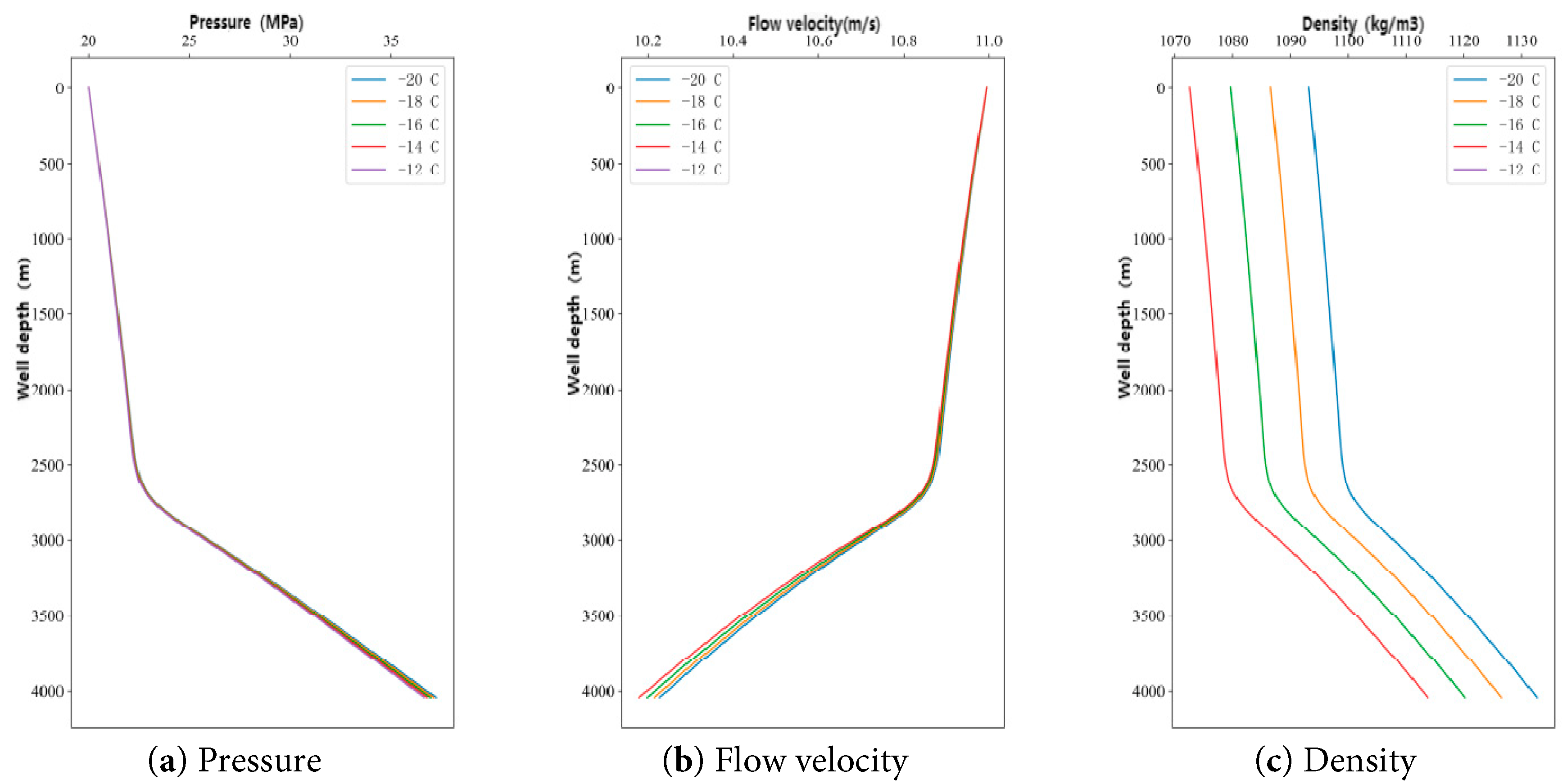
Figure 11: Variation curve of CO₂ fluid properties in casing with well depth.

3.2.3 Wellhead Pressure Changes

By changing the wellhead pressure, the wellbore pressure and temperature are compared. Setting the wellhead pressures of 15 MPa, 20 MPa, 25 MPa, 30 MPa and 35 MPa, the discharge velocity was 8 m3/min, and the wellhead temperature was −15°C. The changes of temperature, pressure, flow velocity and density parameters at different wellhead pressures were obtained respectively, and the variation results are shown in Fig. 12 and Fig. 13.

Fig. 12 shows the temperature variation curves of the wellbore casing, casing inner wall, and cement ring with well depth under different wellhead pressures during CO2 fracturing. From the figure, it can be seen that changes in wellhead pressure do not significantly affect the temperature distribution within the wellbore.

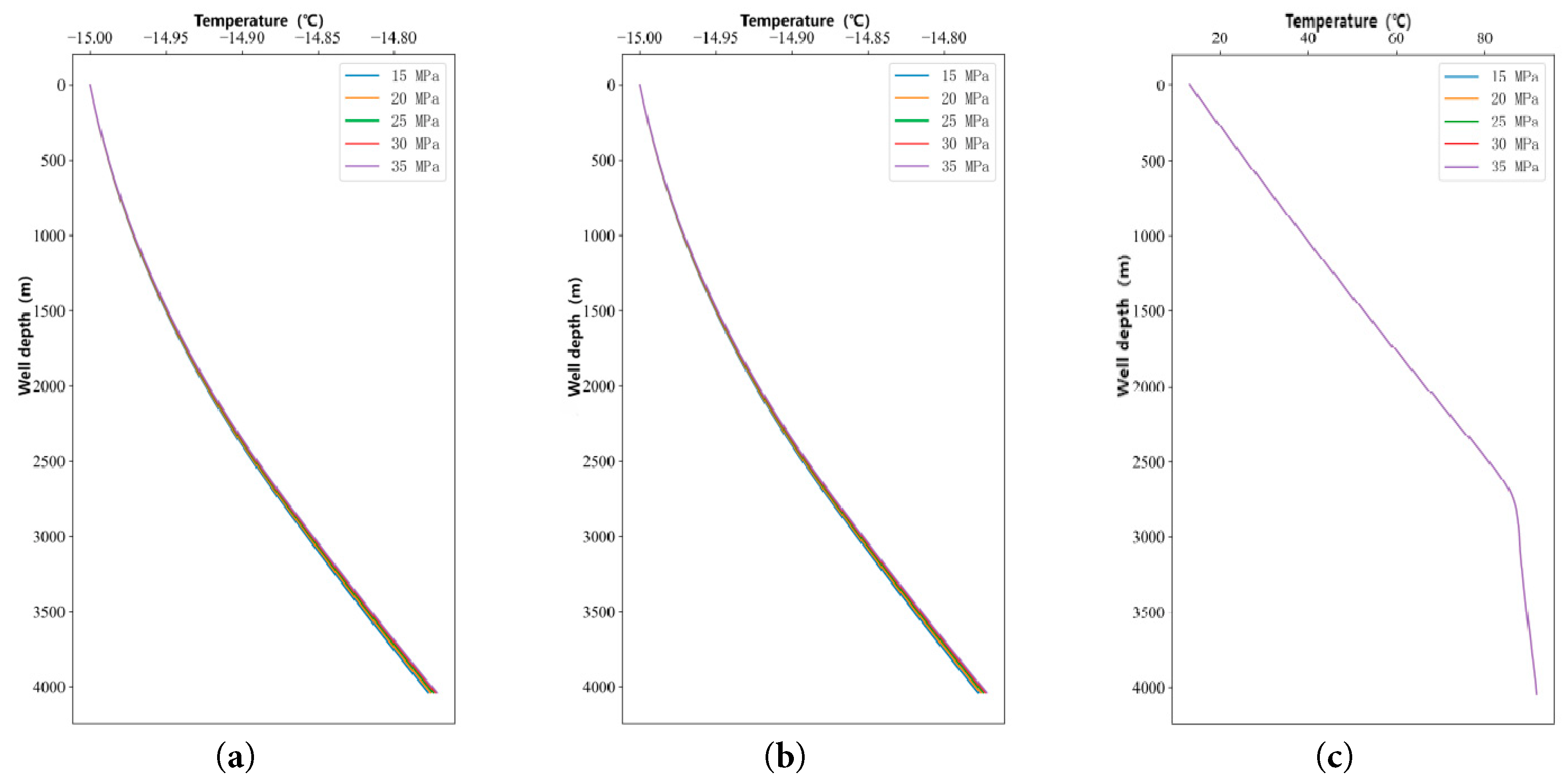
Figure 12: Variation of temperature in various parts of the wellbore with well depth. (a) Casing temperature; (b) Casing inner wall temperature; (c) Temperature of the cement sheath.

Fig. 13 shows the variation curves of CO2 fluid characteristics within the casing with depth under different wellhead pressures. With the change of fracturing fluid pressure injected at the wellhead, the trend of pressure change in the tubing is consistent. The higher the density of the pressure, the higher the velocity of pressure increase in the horizontal section is that in the vertical section. Due to the increase in density, the flow velocity of the medium within the pipe in the horizontal section decreases under the same flow velocity, with the maximum difference approaching 0.4 m/s.

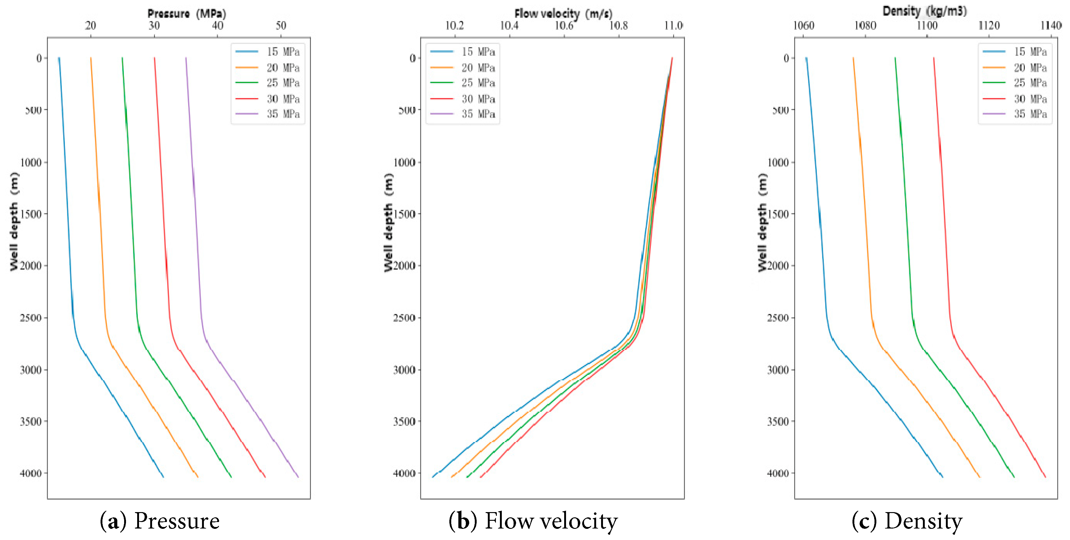
Figure 13: Variation curve of CO₂ fluid properties in casing with well depth.

3.2.4 Fracturing Displacement Changes

By changing the fracturing displacement, the wellbore pressure and temperature are compared. Setting the range of displacement: 2 m3/min, 4 m3/min, 6 m3/min, 8 m3/min, 10 m3/min, wellbore temperature −15°C, wellbore pressure 20 MPa. The changes of temperature, pressure, flow velocity and density parameters under different wellbore pressures were obtained respectively, and the results of the changes are shown in Fig. 14 and Fig. 15.

Fig. 14 shows the temperature variation curves of the casing, the inner wall of the casing, and the cement ring with well depth under different fracturing flow rates during CO2 fracturing. The temperature inside the casing and the casing wall temperature varied consistently, which was mainly affected by convection. At 10 min, the injection of 2 m3/min reaches approximately 1500 m, and the injection of 4 m3/min reaches approximately 3300 m. In the area where the fracturing fluid flows, the temperature rapidly decreases from the formation gradient temperature to the fluid temperature. The temperature of the cement ring decreases step by step with well depth during the process of increasing the displacement. Among them, the temperature drop is most significant in the build-up and horizontal sections at injection rates of 2–6 m3/min, while the temperature drop weakens at rates greater than 8 m3/min.

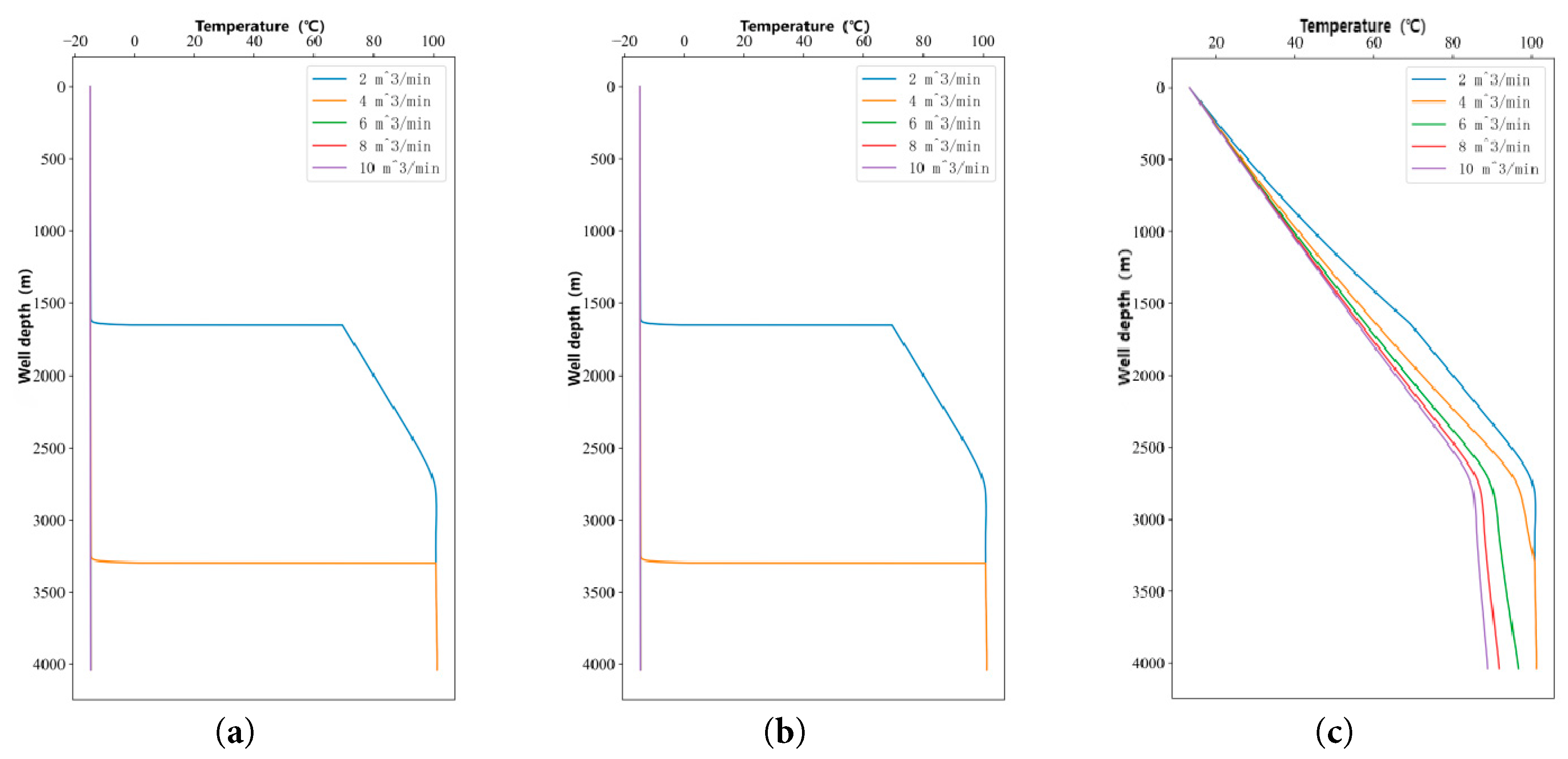
Figure 14: Variation of temperature in various parts of the wellbore with well depth. (a) Casing temperature; (b) Casing inner wall temperature; (c) Temperature of the cement sheath.

Fig. 15 shows the variation curves of CO2 fluid characteristics within the casing with depth under different CO2 fracturing flow rates. After changing the fracturing displacement, the pressure, flow velocity and density changes exhibit greater complexity. Among them, 2 m3/min and 4 m3/min did not flow into the wellbore at 10 min, so the pressure, flow velocity and density remained unchanged. 6 m3/min, 8 m3/min and 10 m3/min flowed into the wellbore at 10 min, in which the pressure and density of the straight section decreased slightly with the increase of fracturing discharge, and the change of flow velocity was insignificant; the change of pressure and density of the diagonal section and the horizontal section increased significantly, and the change of pressure and density of the vertical section and the horizontal section was not obvious. Under the conditions of 8 m3/min and 10 m3/min, the pressure at the bottom of the well reaches up to 35 MPa and 55 MPa, the flow velocity decreases by about 0.5 m/s, and the density increases by about 20 kg/m3.

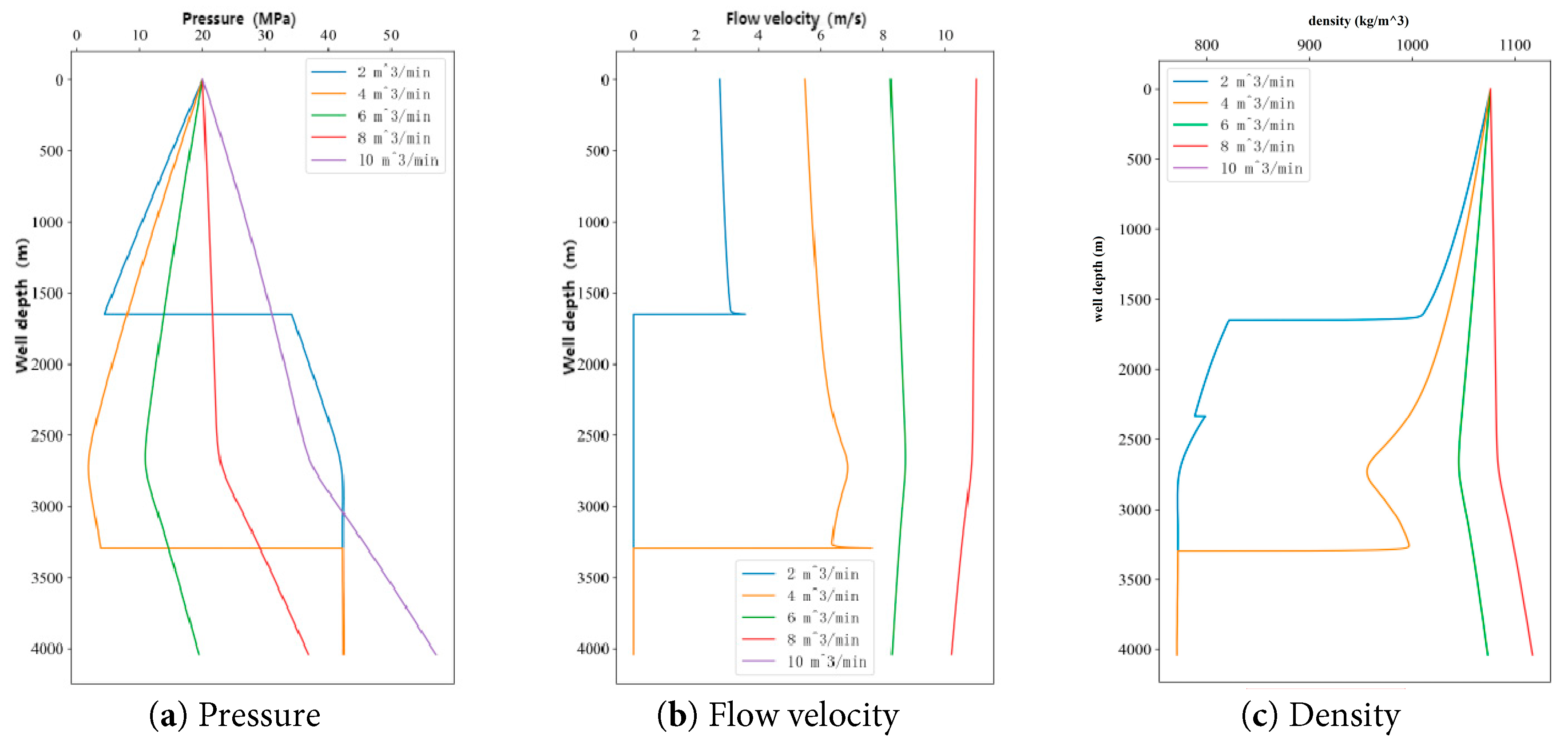
Figure 15: Variation curve of CO₂ fluid properties in casing with well depth.

3.2.5 Changes in the Ground Temperature Gradient

By changing the formation temperature gradient, the wellbore pressure and temperature are compared. Setting the range of formation temperature gradient: 1.5°C/100 m, 2.0°C/100 m, 2.5°C/100 m, 3.0°C/100 m, 3.5°C/100 m, wellbore pressure of 20 MPa, discharge velocity of 8 m3/min and wellbore temperature of −15°C. The changes of temperature, pressure, flow velocity and density parameters under different formation temperature gradients were obtained respectively, and the variation results are shown in Fig. 16 and Fig. 17.

Fig. 16 shows the temperature variation curves of different parts within the wellbore with depth under different ground temperature gradients. When the ground temperature gradient changes, the temperature changes in the casing and the inner wall of the casing are the same. As the temperature gradient of the formation increases, the temperature at the bottom of the well also increases. However, due to the influence of convection, the impact on the formation temperature is minimal. The temperature of the cement sheath gradually increases with the formation temperature gradient.

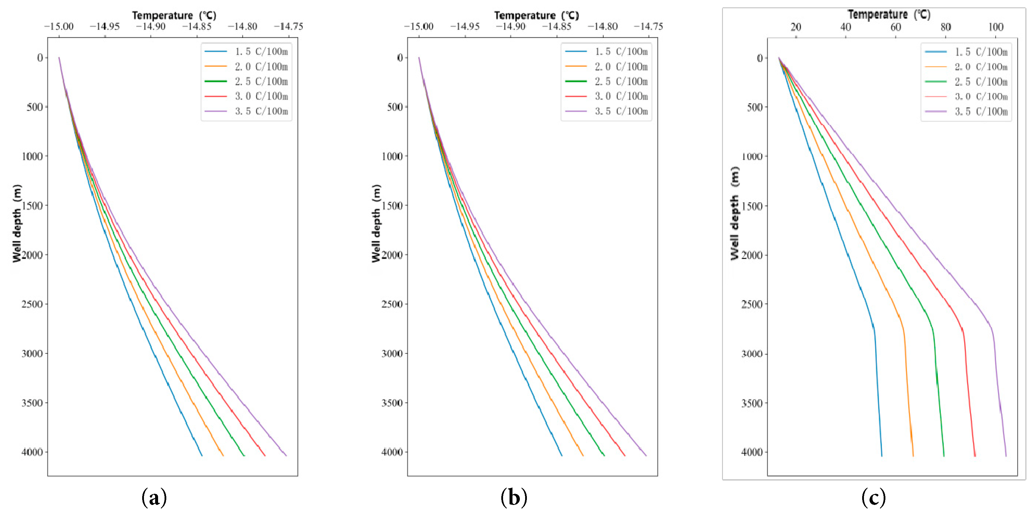
Figure 16: Variation of temperature in various parts of the wellbore with well depth. (a) Casing temperature; (b) Casing inner wall temperature; (c) Temperature of the cement sheath.

Fig. 17 shows the variation curves of CO2 fluid characteristics in the casing with well depth under different formation temperature gradients. From the figure, it can be seen that the effect of ground temperature gradient on the pressure, flow velocity and density of CO2 fluid in the casing is not significant and almost negligible.

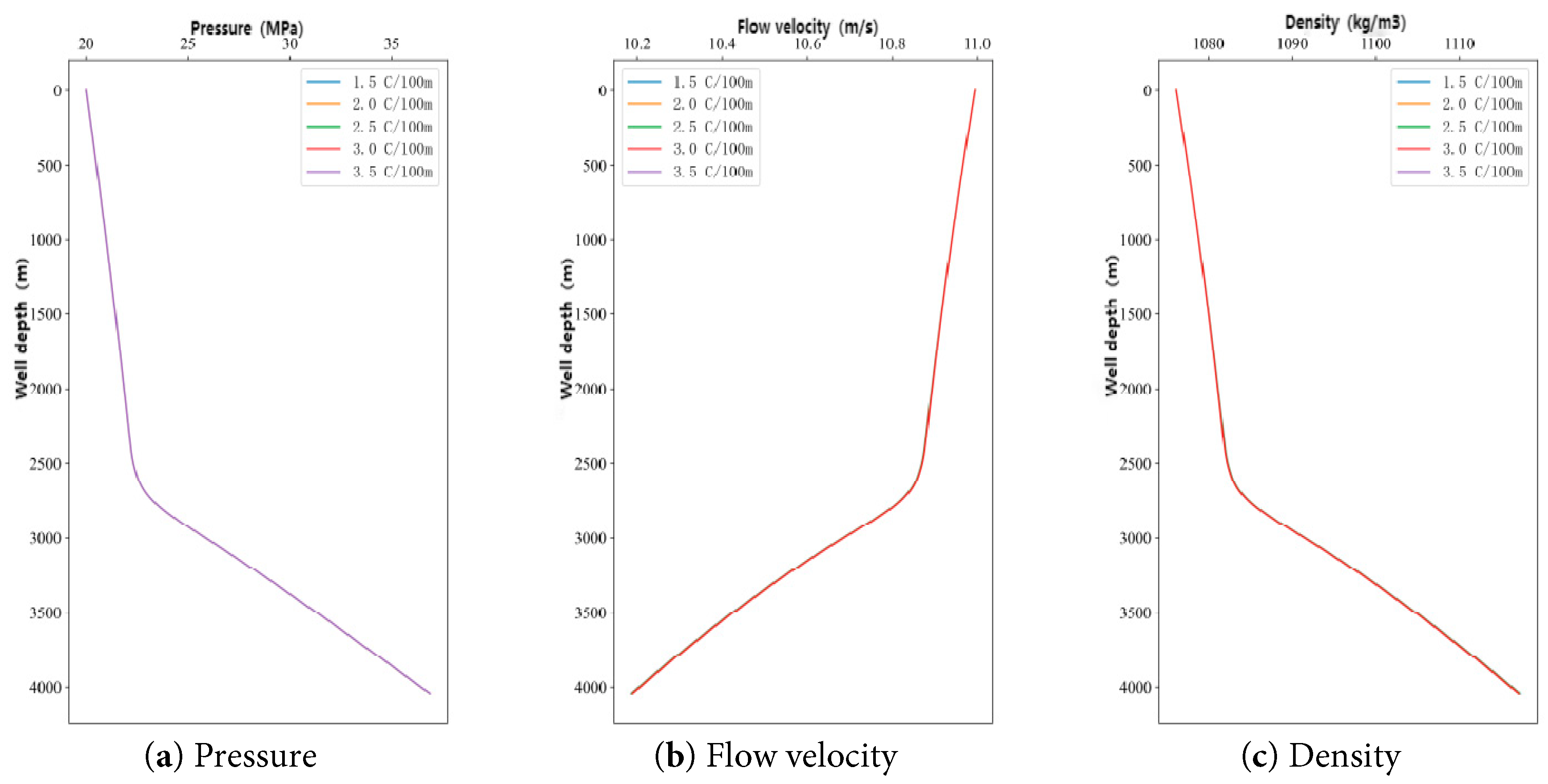
Figure 17: Variation curve of CO₂ fluid properties in casing with well depth.

The above experimental simulations indicate that during the CO2 fracturing process, the changes of injection time, fracturing displacement and ground temperature gradient have a significant impact on the wellbore temperature. As the injection time and fracturing flow velocity increase, the temperature at the bottom of the wellbore gradually decreases; as the ground temperature gradient increases, the temperature at the bottom of the wellbore gradually increases. However, the effects of wellhead temperature and wellhead pressure on the wellbore temperature are small, which is due to the fact that small changes in wellhead temperature have limited effects on the sensible heat of CO2, especially in the high-temperature wellbore region, where the expansion of CO2 is mainly through heat absorption and vaporization, and the latent heat of phase change buffers the temperature change; In the energy conservation equation within the wellbore, the contributions of pressure work and frictional heat to temperature are far less than those of formation heat transfer and convective heat transfer. Therefore, pressure changes primarily affect heat transfer indirectly by altering CO2 density and flow velocity rather than directly changing temperature.

Changes in wellhead temperature and wellhead pressure have a large impact on the CO2 fluid properties in the casing. With the increase of wellhead temperature, the pressure of CO2 in the tubing gradually increases while the flow velocity and density gradually decrease. At a wellhead temperature of −20°C, the bottom hole density reaches 1132 kg/m3. With the increase of wellhead pressure, the flow velocity of CO2 in the tubing decreases while the pressure and density gradually increase. When the wellhead pressure reaches 35 MPa, the wellhead density reaches 1138 kg/m3.

3.2.6 Carbon Dioxide Phase Prediction in the Wellbore

The phase change of CO2 is very complex. In the CO2 dry fracturing operation, as shown in Fig. 18, the initial CO2 is stored in a liquid state in the CO2 tanks. After pressurization, the liquid CO2 is pumped into the high-pressure pump. At the outlet of the pump truck, the liquid CO2 is injected into the bottom of the well after being pressurized. During this process, the pressure continuously increases, and the temperature correspondingly rises. When the liquid CO2 flows into the fracture of the formation, the pressure and temperature of the formation will assimilate the liquid CO2, which will make the temperature of the liquid CO2 increase and its pressure decrease, and then the liquid CO2 will be transformed into supercritical CO2. After the end of the dry fracturing operation, the fracturing fluid needs to be returned to the drain, and the pressure will decrease, which will transform the supercritical CO2 into a gas and discharge it from the ground.

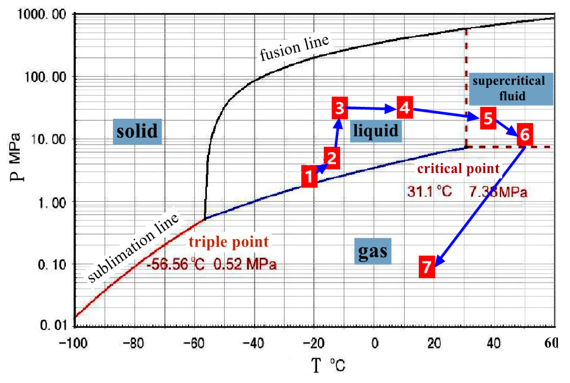
Figure 18: Schematic diagram of phase change of CO₂ during dry fracturing process.

The key value between temperature and pressure on the change of phase state is density. By predicting CO2 phase state changes through different densities at varying pressures and temperatures. The variation of density with temperature and pressure is shown in Fig. 19. As can be seen in Fig. 19a, the higher the pressure, the slower the change in CO2 density with temperature until it approaches a linear change. Fig. 19b shows the CO2 density at different temperatures with the pressure change curve showing that if the CO2 temperature is lower than the critical temperature, the pressure is lower, and CO2 is in the gas state, and the density is small. With the increase of pressure, when the pressure > CO2 saturation vapor pressure, gaseous CO2 becomes liquid CO2, resulting in a sudden increase in its density. When the temperature is above the critical temperature, the density of CO2 increases rapidly. The density of CO2 near the critical point has a high sensitivity to changes in temperature and pressure, and in the near-critical region, small changes in temperature or pressure can lead to significant changes in CO2 density.

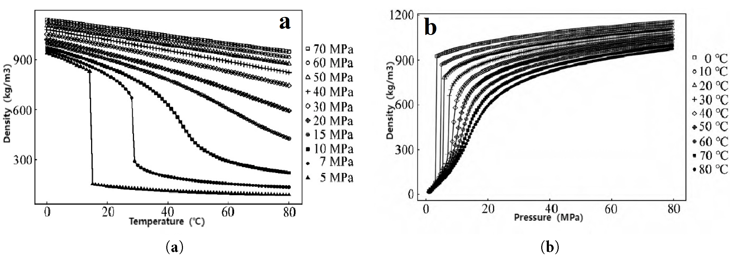
Figure 19: CO₂ density variation curve with temperature and pressure. (a) CO₂ density versus temperature at different pressures; (b) CO₂ density versus pressure at different temperature.

The simulation results of the temperature and pressure inside the wellbore are shown in Fig. 20. During the CO2 injection process, low-temperature liquid CO2 is injected into the wellhead, while the temperature of the formation’s isothermal zone is higher than the temperature of the injected CO2. As a result, the formation continuously heats the CO2 within the wellbore. This causes the temperature in the wellbore to increase with the depth of the wellbore. Over time, the temperature at various locations in the wellbore gradually decreases due to the continuous injection of low-temperature CO2 into the wellbore.

Wellbore pressure continuously decreases with increasing wellbore depth and gradually increases with the extension of the injection construction time. Compared to CO2 drive/seal injection, the injection volume and injection pressure of the CO2 fracturing process are much larger. At this time, the CO2 flow velocity in the wellbore is relatively high, and the main controlling factor of the wellbore pressure is not gravity, but the frictional losses caused by the flow, so the wellbore pressure gradually decreases.

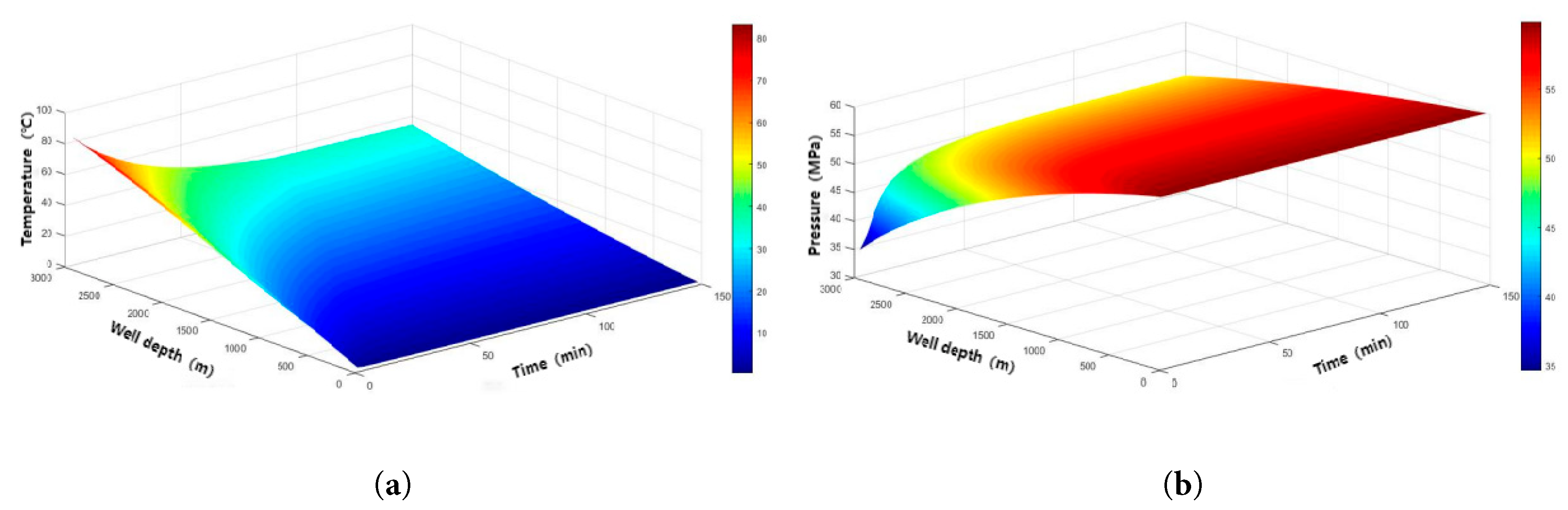
Figure 20: Temperature and pressure distribution in the wellbore. (a) Temperature distribution along the depth of the wells; (b) Pressure distribution along the depth of the wells.

Through the research on CO2 parameters, it is known that density, viscosity, and thermal conductivity decrease continuously with the decrease in temperature, while specific heat and Joule-Thomson coefficient increase with the increase in temperature [22]. As shown in Fig. 21, the distribution cloud map intuitively demonstrates the significant differences in the changes of thermal physical parameters with depth in the wellbore overtime during the CO2 sequestration injection process. During the injection construction process, the density, viscosity and thermal conductivity of CO2 show significant differences, but their trends are similar. At the beginning of injection, the heat capacity and Joule-Thomson coefficient at the bottom of the well fluctuated significantly. This is because when liquid CO2 transitions to a supercritical state, its heat capacity increases sharply, and after reaching the supercritical state, the change in CO2’s heat capacity becomes more gradual. The calculations show that if the fluid physical property parameters are regarded as constants when calculating the temperature and pressure distribution in the wellbore, it will result in significant computational errors. Therefore, they should be treated as variables during the calculations.

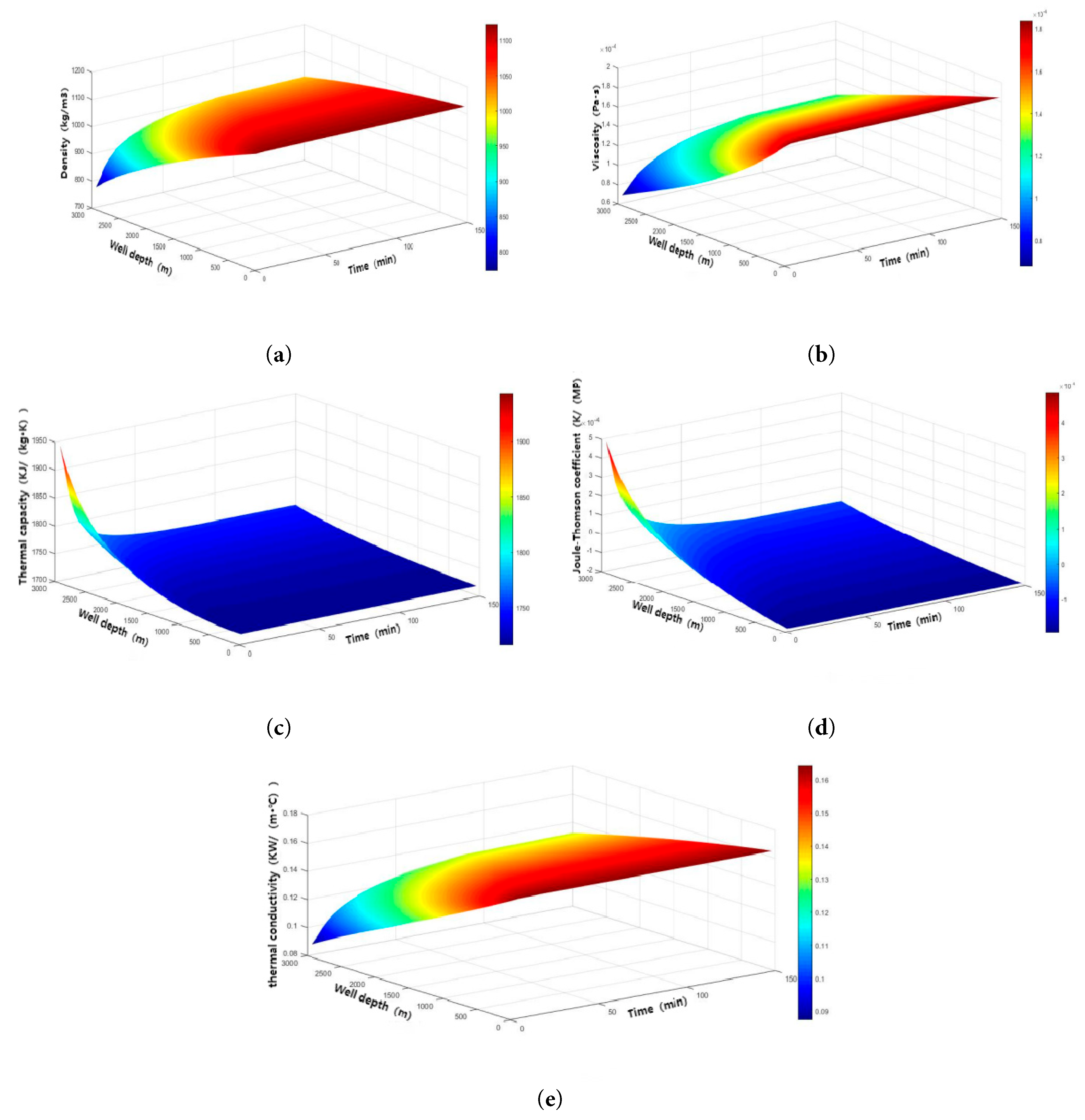
Figure 21: Distribution of thermophysical parameters in CO₂ injected wellbore. (a) Density distribution along well depths; (b) Viscosity distribution along well depths; (c) Heat capacity distribution along well depths; (d) Joule-Thomson coefficient distribution along well depths; (e) Thermal conductivity distribution along well depths.

Summarizing the data on the temperature and pressure changes with depth in the wellbore at different times and comparing it with the CO2 phase diagram to visually analyze the phase transition process of CO2 in the wellbore. The summary plot is shown in Fig. 22. Due to the high pressure injected during the fracturing process, friction becomes the dominant factor affecting the temperature and pressure distribution in the wellbore, leading to an increase in temperature and a continuous decrease in wellbore pressure. The data were collated to obtain a schematic diagram of the location of the phase transition in the wellbore in Fig. 23. From the diagram, it can be seen that during the initial stage of injection, low-temperature liquid CO2 is injected into the wellbore. At this time, the formation heats the CO2 within the wellbore, causing its temperature to rapidly rise above the critical temperature, resulting in a phase transition. As the injection process continues, the temperature within the wellbore will decrease over time due to the continuous injection of low-temperature liquid CO2. This leads to the position of the phase transition moving continuously downward in the wellbore. When the injection time reaches 90 min or more, the heat transfer process in the wellbore gradually stabilizes, and the temperature no longer changes significantly. Correspondingly, the depth of the CO2 phase transition gradually stabilizes at a depth of 2790 m. However, it is important to note that the temperature changes within the wellbore do not actually reach a true steady state, so the phase transition position only reaches a dynamic equilibrium state.

The current model assumes a fixed pressure boundary (fracture closure pressure) at the bottom of the well, but actual reservoir seepage may lead to dynamic pressure changes. If the outlet is changed to a reservoir seepage boundary (e.g., Darcy’s law coupling), liquid CO2 may gasify rapidly in the near-well zone due to a pressure drop to saturated vapor pressure, triggering local cooling. In addition, seepage resistance may keep the horizontal section pressure higher than currently predicted, delaying the transition of CO2 to the supercritical state. Future work needs to couple reservoir seepage models to quantify the effect of dynamic boundaries on wellbore thermodynamic parameters.

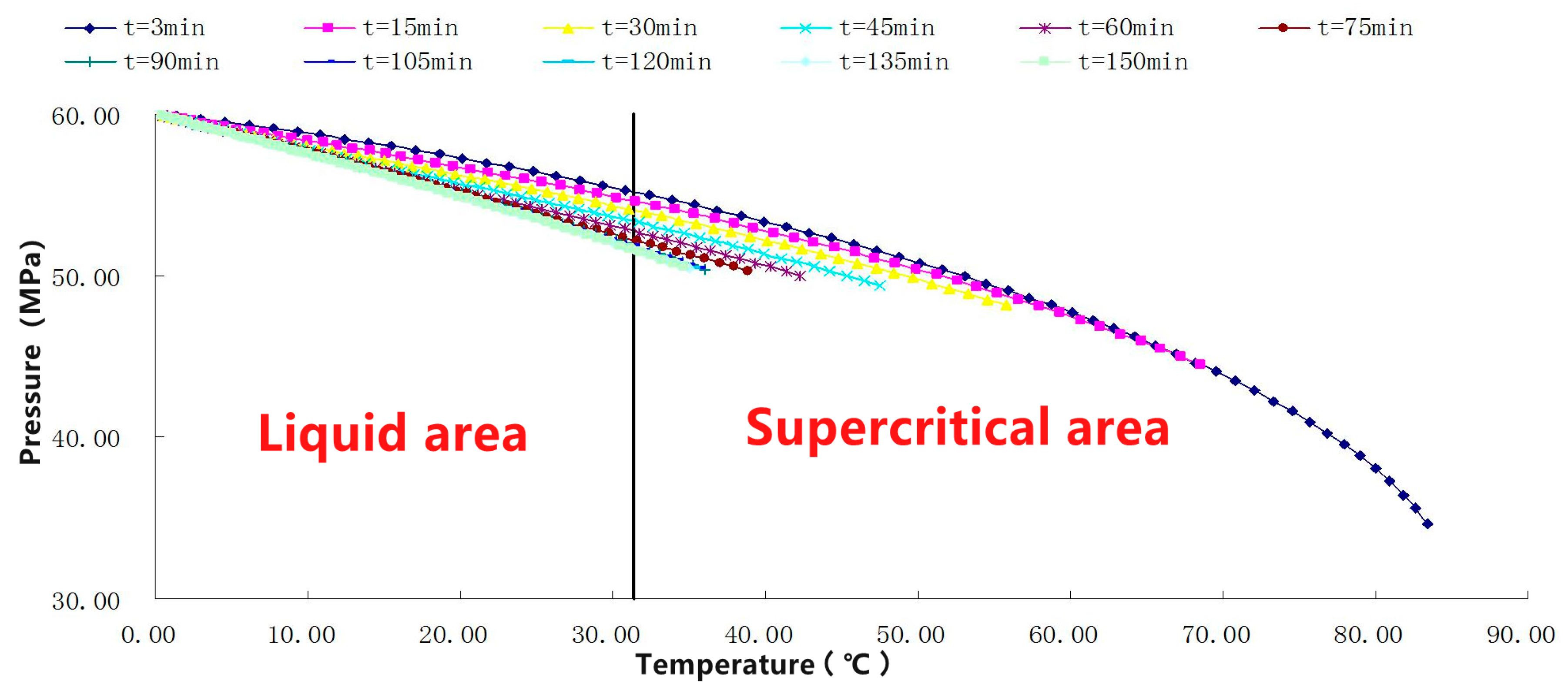
Figure 22: Phase distribution of liquid CO₂ injection wellbore.

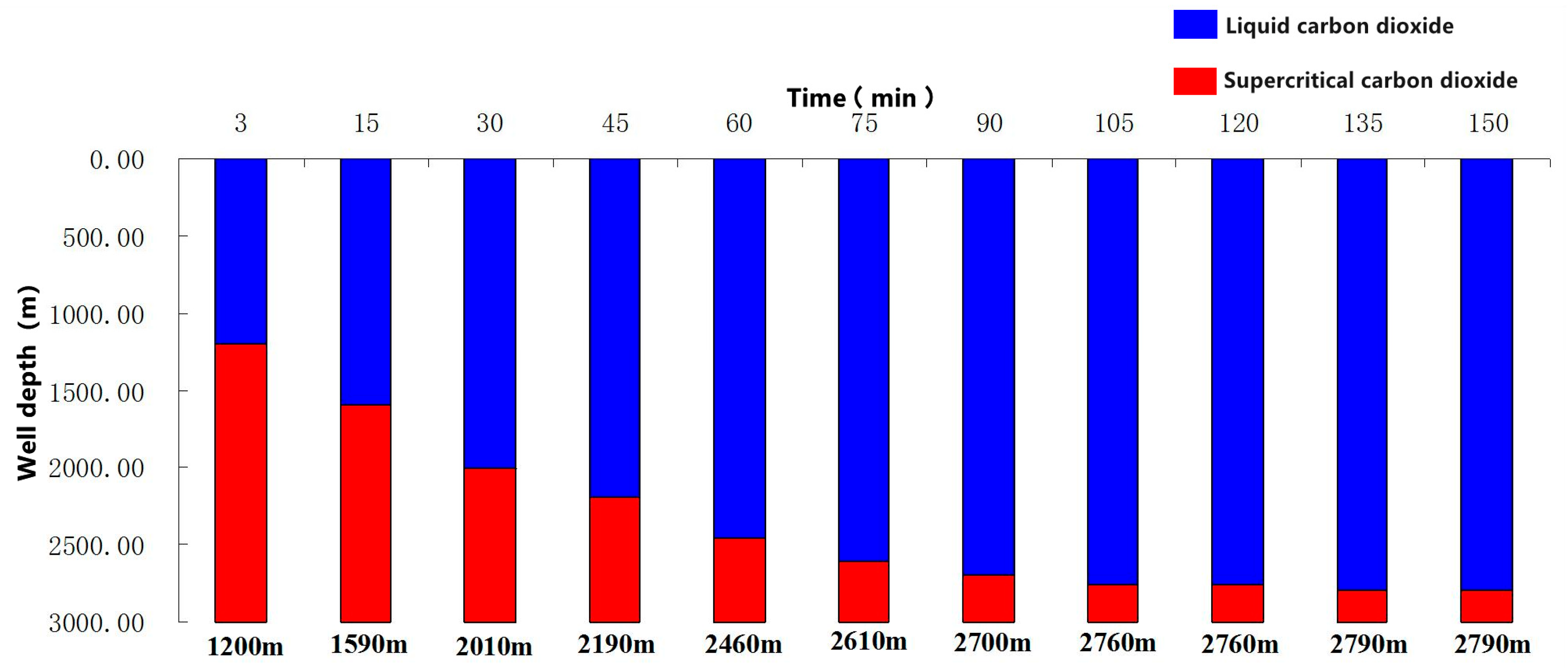
Figure 23: Schematic diagram of the phase transition process of liquid CO₂ injection into the wellbore.

4 Conclusion

In this paper, a two-dimensional unsteady flow and thermal conductivity model is established for the temperature variation of CO2 fracturing wellbore. It considers high-speed flow within the pipe and radial heat transfer in the wellbore. Python is used for coding and solving, and it derives the temperature, pressure, flow velocity, and medium density at different times in the fracturing wellbore and formation, thereby predicting the phase state of CO2 within the wellbore.

• (1)After the low-temperature CO2 fracturing fluid is injected into the tubing, a radial temperature gradient of less than 10 cm gradually forms in the annulus, casing, and cement ring. When the fracturing fluid flows through the entire tubing section, a relatively stable radial temperature gradient is formed. The temperature gradient at the far end of the formation is the preset value and is less affected by the low-temperature medium in the wellbore. In the vertical well section, the temperature of the CO2 increases by approximately 8°C, leading to volume expansion and increased pressure; however, the changes in medium density and flow velocity are not significant. In the horizontal section, the temperature of the cement ring in the wellbore tends to stabilize. However due to the high-temperature environment in the horizontal section, CO2 continues to absorb heat and expand, resulting in a significant increase in pressure (from 48 MPa to 68 MPa), an increase in density, and a decrease in flow velocity.
• (2)This paper combines one-dimensional axial non-isothermal flow with one-dimensional radial unsteady heat transfer to establish a two-dimensional temperature-pressure coupling model. The model is discretized using a fully implicit finite difference method, and Python is used for coding and solving. Parameters such as inlet temperature, inlet pressure, fracturing flow velocity, and formation temperature gradient are selected as variables for model analysis, leading to the following conclusions:
  • ➀Influenced by the high-speed convection of fracturing fluid in the tubing, the temperature distribution in the wellbore is greatly influenced by the injection time, fracturing displacement, and ground temperature gradient but is less affected by the wellhead temperature and pressure;
  • ➁The pressure distribution in the wellbore is greatly influenced by the wellhead pressure;
  • ➂The CO2 flow velocity in the wellbore is greatly influenced by the fracturing displacement;
  • ➃The density of CO2 in the wellbore is greatly affected by the wellhead temperature and wellhead pressure. When the wellhead temperatures are −20°C and −14°C, the density values are 1132 kg/m3 and 1092 kg/m3, respectively. When the wellhead pressures are 30 MPa and 15 MPa, the density values are 1142 kg/m3 and 1082 kg/m3, respectively.

• (3)A real-time phase transition depth prediction method based on density gradient judgment is developed, which improves the accuracy of phase transition position prediction compared to the traditional P-T intercept method. According to the above prediction method, it is concluded that CO2 will be transformed from a liquid state to a supercritical state during injection into the wellbore. As the injection progresses, the depth of the transition to the supercritical state gradually moves towards the bottom of the well. In the early stages of injection, the depth of the transition to the supercritical state changes rapidly, but as the injection continues, the depth of the transition to the supercritical state gradually stabilizes. During the phase transition process, the thermophysical parameters of CO2 change significantly, especially at the critical point, where small variations in temperature and pressure can lead to abrupt changes in density.

References

1. Xia YL, Li L, Wang Z. Experimental and numerical study on influencing factors of replacement capacity and slickwater flowback efficiency using pre-CO2 fracturing in tight oil reservoirs. J Pet Sci Eng. 2022;215(Part B):110697. doi:10.1016/J.PETROL.2022.110697. [Google Scholar] [CrossRef]
2. Ramey HJ. Wellbore heat transmission. J Pet Technol. 1962;14(4):427–35. [Google Scholar]
3. Wu HQ, Bai B, Li XC, Liu M, He Y. An explicit finite difference model for prediction of wellbore pressure and temperature distribution in CO2 geological sequestration. Greenh Gases Sci Technol. 2017;7(2):353–69. doi:10.1002/ghg.1647. [Google Scholar] [CrossRef]
4. Arnold FC. Temperature variation in a circulating wellbore fluid. J Energy Resour Technol. 1990;112(2):79–83. doi:10.1115/1.2905726. [Google Scholar] [CrossRef]
5. Alves IN, Alhanati FJS, Shoham O. A unified model for predicting flowing temperature distribution in wellbores and pipelines. SPE Prod Eng. 1992;7(4):363–7. doi:10.2118/20632-pa. [Google Scholar] [CrossRef]
6. Hasan AR, Kabir CS. Heat transfer during two-phase flow in wellbores; part I—formation temperature. In: Proceedings of the SPE Annual Technical Conference and Exhibition; 1991 Oct 6–9; Dallas, TX, USA. doi:10.2523/22866-ms. [Google Scholar] [CrossRef]
7. Hasan AR, Kabir CS, Lin D. Analytic wellbore-temperature model for transient gas-well testing. SPE Reserv Eval Eng. 2005;8(3):240–7. doi:10.2118/84288-pa. [Google Scholar] [CrossRef]
8. Gu H, Cheng L, Huang S, Du B, Hu C. Prediction of thermophysical properties of saturated steam and wellbore heat losses in concentric dual-tubing steam injection wells. Energy. 2014;75:419–29. doi:10.1016/j.energy.2014.07.091. [Google Scholar] [CrossRef]
9. Lv XR. Study on the temperature field of horizontal wellbores during CO2 fracturing in shalegas reservoirs [dissertation]. Beijing, China: China University of Petroleum; 2019. (In Chinese). doi:10.27643/d.cnki.gsybu.2019.000070. [Google Scholar] [CrossRef]
10. Xiao B. Coupling solving method of temperature and pressure field during supercritical carbon dioxide dry-fracturing. China Sci Technol Pap. 2020;15(1):119–24. (In Chinese). [Google Scholar]
11. Wu L, Luo ZF, Zhao LQ, Yao ZG, Jia YC. Study on wellbore temperature & pressure and phase control in supercritical carbon dioxide fracturing. J Southwest Pet Univ Sci Technol Ed. 2023;45(2):117–25. (In Chinese). [Google Scholar]
12. Yao X, Song X, Zhou M, Xu Z, Duan S, Li Z, et al. A modified heat transfer model for predicting wellbore temperature in ultra-deep drilling with insulated drill pipe. Energy. 2025;331:136981. doi:10.1016/j.energy.2025.136981. [Google Scholar] [CrossRef]
13. Al-Adwani FA. Mechanistic modeling of an underbalanced drilling operation utilizing supercritical carbon dioxide [dissertation]. Baton Rouge, LA, USA: Louisiana State University; 2007. [Google Scholar]
14. Span R, Wagner W. A new equation of state for carbon dioxide covering the fluid region from the triple-point temperature to 1100 K at pressures up to 800 MPa. J Phys Chem Ref Data. 1996;25(6):1509–96. doi:10.1063/1.555991. [Google Scholar] [CrossRef]
15. Yasunami T, Sasaki K, Sugai Y. CO2 temperature prediction in injection tubing considering supercritical condition at yubari ECBM pilot-test. J Can Petrol Technol. 2010;49(4):44–50. doi:10.2118/136684-pa. [Google Scholar] [CrossRef]
16. Ruan B, Xu R, Wei L, Ouyang X, Luo F, Jiang P. Flow and thermal modeling of CO2 in injection well during geological sequestration. Int J Greenh Gas Control. 2013;19:271–80. doi:10.1016/j.ijggc.2013.09.006. [Google Scholar] [CrossRef]
17. Li XJ. Research on flow-heat transfer and rock damage during CO2 fracturing based on multiphysics coupling [dissertation]. Beijing, China: China University of Petroleum; 2018. (In Chinese). doi:10.27643/d.cnki.gsybu.2018.000095. [Google Scholar] [CrossRef]
18. Luo PD, Li HY, Zhai LJ, Li CY, Lv XR, Mou JY. Supercritical CO2 fracturing wellbore and fracture temperature field in Tahe Oilfield. Fault-Block Oil Gas Field. 2019;26(2):225–30. (In Chinese). [Google Scholar]
19. Guo X, Sun X, Mu JF, Qiao HJ, Luo P, Li P. Heat transfer in wellbores fractured with supercritical CO2 fracturing fluid. Drill Fluid Complet Fluid. 2021;38(6):782–9. (In Chinese). [Google Scholar]
20. Li N, Yu J, Zhang H, Zhang Q, Kang J, Zhang N, et al. Simulation of wellbore temperature and pressure field in supercritical carbon dioxide fracturing. Petrol Sci Technol. 2024;42(2):190–210. doi:10.1080/10916466.2022.2116047. [Google Scholar] [CrossRef]
21. Sang RL. Study on wellbore thermal-fluid coupling mechanism of CO2 fracturing in horizontal wells of shale gas reservoirs [master’s thesis]. Daqing, China: Northeast Petroleum University; 2023. (In Chinese). doi:10.26995/d.cnki.gdqsc.2023.000947. [Google Scholar] [CrossRef]
22. Gao X, Yang S, Shen B, Wang J, Tian L, Li S. Effects of CO2 variable thermophysical properties and phase behavior on CO2 geological storage: a numerical case study. Int J Heat Mass Transf. 2024;221:125073. doi:10.1016/j.ijheatmasstransfer.2023.125073. [Google Scholar] [CrossRef]
23. Tang LH, Yang BH, Pan J, Sundén B. Thermal performance analysis in a zigzag channel printed circuit heat exchanger under different conditions. Heat Transf Eng. 2022;43(7):567–83. doi:10.1080/01457632.2021.1896832. [Google Scholar] [CrossRef]
24. Chen NH. An explicit equation for friction factor in pipe. Ind Eng Chem Fund. 1979;18(3):296–7. doi:10.1021/i160071a019. [Google Scholar] [CrossRef]
25. Bergman TL. Fundamentals of heat and mass transfer. 4th ed. Hoboken, NJ, USA: John Wiley & Sons, Inc.; 2011. 1048 p. [Google Scholar]
26. Zhao XB, Yang N, Liang H, Wei M, Ma B, Qiu D. The wellbore temperature and pressure behavior during the flow testing of ultra-deepwater gas wells. Fluid Dyn Mater Process. 2024;20(11):2523–40. doi:10.32604/fdmp.2024.052766. [Google Scholar] [CrossRef]
27. Lurie MV. Modeling of oil product and gas pipeline transportation. Hoboken, NJ, USA: John Wiley & Sons, Inc.; 2008. 214 p. doi:10.1002/9783527626199. [Google Scholar] [CrossRef]
28. Dropkin D, Somerscales E. Heat transfer by natural convection in liquids confined by two parallel plates which are inclined at various angles with respect to the horizontal. J Heat Transf. 1965;87(1):77–82. [Google Scholar]
Cite This Article
Copyright © 2025 The Author(s). Published by Tech Science Press.
This work is licensed under a Creative Commons Attribution 4.0 International License , which permits unrestricted use, distribution, and reproduction in any medium, provided the original work is properly cited.
Downloads
Citation Tools