1 Introduction
The flow around a cylinder is a classical problem in fluid mechanics. Understanding the flow characteristics is significant for understanding the flow around a blunt body and optimizing the design of engineering structures (e.g., bridges, marine risers, and heat exchangers) [1,2,3]. Due to complex flow interference effects (e.g., vortex shedding and wake interaction), the flow around double cylinders has become a research hotspot in recent years [4].
The flow around a single cylinder forms the basis for studying the surrounding flow. Sahin & Owens [5] found that in the confined case, at a blockage ratio of β = 0.2 , the critical Reynolds number of the transition from steady flow to periodic Karman vortex street rises to about R e c ≈ 69 (for unconfined flow around a single cylinder, R e c ≈ 47 ) due to wall effects. At a high blocking ratio, the wall effect significantly influences the flow, and the asymmetric oscillation increases the lift coefficient fluctuation, which may affect structural stability. Zhang et al. [6] developed a new method combining the lattice Boltzmann method (LBM) and dynamic mode decomposition for stability analysis of flow around a cylinder at R e = 50 . This method efficiently analyzed the periodic and transient flow states resembling harmonic motion. Nie and Lin [7] conducted a numerical analysis of two-dimensional flow past a half cylinder in the two bluff arrangements confined by parallel walls, noting that compared to full cylinders, the critical Reynolds number for flow separation and vortex shedding is lower for a half cylinder. They also highlighted the dominant role of pressure drag at certain Reynolds numbers. Mashhadi et al. [8] conducted numerical studies of two-dimensional and three-dimensional unsteady flow on rectangular cylinders with different aspect ratios ( A R = 0.25–4.0) in the R e = 30–200 range, revealing the effects of A R and R e on flow structure, critical Reynolds number, and separation mechanisms, and providing physical insights into how flow behavior changes with A R and R e . Abdelhamid et al. [9] used numerical simulations to investigate the effects of the corner radius ratio r / R = 0.0–1.0 and Reynolds number R e = 40–180 on the flow around a square cylinder, heat transfer, and aerodynamic forces, revealing four main flow patterns. In terms of flow control, Li and Zhang [10] applied a reinforcement learning (RL)-based flow control strategy to the flow past a cylinder confined between two walls. By controlling two synthetic jets to blow and suction on the cylinder, they successfully suppressed vortex shedding. Li et al. [11] proposed a reduced-order model combining DMD with attention-enhanced CNN-LSTM for efficient and accurate prediction of unstable wake caused by cylinders, significantly reducing computational costs while maintaining CFD accuracy. Al-Sadawi et al. [12] conducted a simulation study on the effect of passive jet control with different slot angles on the flow around a cylinder. They found that at subcritical Reynolds numbers, a 130° slot could significantly improve the pressure distribution and reduce drag by up to 26%, verifying the key role of jet position in flow control. Amini et al. [13] studied the flow and heat transfer characteristics of a power-law fluid around a porous elliptical cylinder using a numerical simulation system, revealing the significant effects of different aspect ratios, Reynolds numbers, power-law exponents, and Darcy numbers on wake structure, vortex type, drag, and heat transfer performance. Ren et al. [14] proposed a deep reinforcement learning (DRL) based spin control strategy for cylinders, achieving a significant 99.6% reduction in amplitude during the lock-in phase, demonstrating the effectiveness and potential of DRL in active control of complex flows.
For the flow around two cylinders, the flow characteristics depend on the arrangement (tandem, side-by-side, and staggered) and spacing ratio ( L / D ). Alam et al. [15] conducted numerical simulations of the flow around four parallel cylinders at R e = 100 based on the finite volume method (FVM), revealing the effects of spacing ratio on flow conditions, aerodynamic forces, and vortex shedding patterns. They identified four typical wake structures and found that the total time-averaged drag and repulsive force increased exponentially as the spacing decreased. Alam [16] studied flow-induced vibrations caused by wake interference between two cylinders at R e = 150, revealing the complex effects of mass ratio, damping ratio, and spacing on the vibration response. He pointed out that the mass ratio has a more significant effect on amplitude than the damping ratio, and that wake structure plays a key role in the vibration mechanism. Ahmad et al. [17] used the LBM to simulate two-dimensional flow through a tandem rectangular cylinder at R e = 100, revealing the significant influence of aspect ratio and gap on flow patterns, force characteristics, and spectral structure. They identified five typical flow patterns and determined key critical parameters. Kalsoom et al. [18] used the LBM to study the two-dimensional flow characteristics of two square cylinders with control rods at R e = 150, revealing the significant influence of control rod length on flow patterns, aerodynamic forces, and Strouhal numbers. They identified four types of flow patterns and quantified the variation rules of drag and lift. Gul et al. [19] used the LBM method to study two horizontally placed staggered rectangles and identified seven flow patterns. Ali et al. [20] found that cylinder arrangement significantly affects flow separation, vortex shedding, and heat transfer, with the staggered configuration providing superior thermal performance compared to tandem and side-by-side layouts.
This study used an LBM numerical simulation to investigate the phenomenon of staggered two-cylinder flow around a confined basin under steady flow and vortex-shedding conditions. The Reynolds number range is 0.1 ≤ R e ≤ 160 . The flow is expected to be laminar and two-dimensional for R e in this range. Emphasis is placed on analyzing the effects of different T / D and L / D values of the staggered two-cylinder on the force characteristics, vortex shedding frequency, and tail vortex patterns of the cylinder structure.
2 Method and Problem Description
2.1 Lattice Boltzmann Method
The Lattice Boltzmann Method (LBM) is a computational approach based on the kinetic theory of gases and can be regarded as a mesoscopic alternative to solving the Navier–Stokes equations. It originates from the Boltzmann equation, which governs the evolution of the single-particle distribution function f x , ξ , t ( ξ is the particle velocity vector, x is the spatial position vector, and t is the time) in phase space [21]. By approximating the single-relaxation time (SRT), the Boltzmann equation can be simplified to the Bhatnagar–Gross–Krook (BGK) model [22]: ∂f∂t+ξ·∇f=−1λf−f0(1) where f 0 is the equilibrium distribution function (the Maxwell–Boltzmann distribution function). λ is the relaxation time, which is related to fluid viscosity by the equation v = λ R T , where R is the gas constant and T is the gas temperature. To develop a numerical scheme suitable for CFD, the equation is discretized in velocity space using a finite set of discrete velocities ξ α . This leads to the discretized Boltzmann equation [23]:
∂fα∂t+ξα·∇fα=−1τfα−fαeq(2) In the above equation, f α x , t represents the particle distribution function along the discrete velocity direction ξ α , ???? is the dimensionless relaxation time, and f α e q is the corresponding discrete equilibrium distribution function. This discretization forms the theoretical foundation of the LBM.
In the LBGK model [24] used in this study, Eq. (2) is discretized in a very special manner. The completely discretized equation, with the time step Δ t and space step Δ x = e i Δ t , is fix+eiΔt,t+Δt−fix,t=−1τfix,t−fieqx,t(3) where f i x , t is the distribution function of the microscopic velocity e i at position x and time t . The equilibrium distribution function f i e q x , t describes the distribution of fluids in a local equilibrium state, as follows: fi eqx,t=wiρ1+3ei·ucs2+9ei·u22cs4−3u22cs2(4) c s is the speed of sound; in this study, c s = c / 3 . w i is a weight factor related to the grid model used. In this study, the D2Q9 model (Fig. 1) was used, and the corresponding w i values were w0 = 4/9, w1–4 = 1/9, and w5–8 = 1/36. The velocity vector is expressed as follows:
ei=0,0,for i=0±1,0c, 0,±1c,for i=1 to 4±1,±1c,for i=5 to 8(5) 
Figure 1: D2Q9 lattice model.
Specifically, the lattice speed is c = Δ r / Δ t . A grid spacing of Δ r = 1 and unit lattice time of Δ t = 1 were used in this study.
From the distribution function f i x , t and the velocity vector e i , the macroscopic density ρ and velocity u of the fluid can be calculated:
ρ=∑ifi, ρu=∑ifiei(6) The fluid density is set as ρ = 1 . The dynamic viscosity is set as μ = ρ ν , where ν denotes the kinematic viscosity.
By applying the Chapman-Enskog expansion, the macroscopic mass and momentum equations for the low-Mach limit can be obtained from Eq. (1).
∂ρ∂t+∇·ρu=0(7) ∂ρu∂t+∇·ρuu=−∇p+∇·ρν∇u+∇uT(8) 2.2 Problem Definition
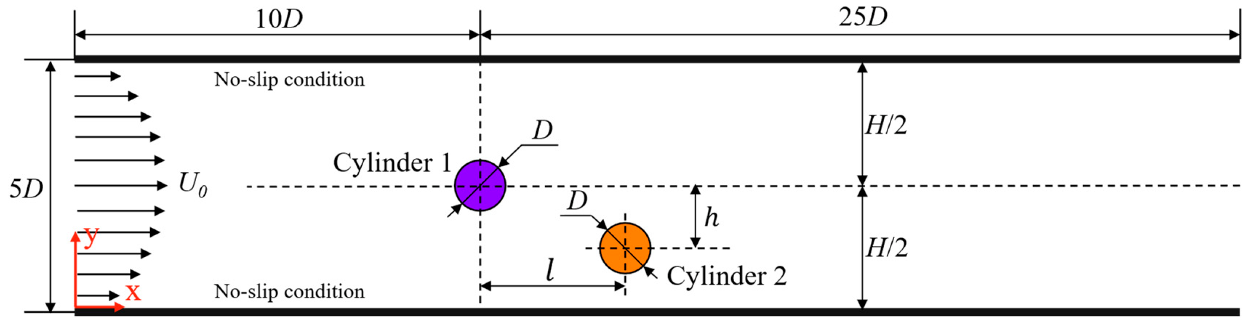
Fig. 2 shows the double-cylinder arrangement and calculation domain used in this study. The two cylinders have a diameter D = 40 Δ x , and the calculated domain size is 35 D × 5 D . Cylinder 1 was fixed at the center of symmetry of the parallel wall, 10 D from the inlet and 25 D from the outlet. Because of symmetry, this study only considered the case where cylinder 2 was placed below the back side of cylinder 1, defining the horizontal distance between the centers of the two cylinders as l and the vertical distance as h (Table 1). The inlet boundary condition was set to a prescribed parabolic inflow, and the outlet boundary condition was set to a fully developed flow. The parabolic equation for the inlet flow rate is as follows: uin=U01−1−2y/H2(9) where U 0 represents the inlet center velocity, and H represents the inlet height. The Reynolds number in this study is based on the inlet velocity boundary and is defined as:
Re=U0Dv(10) 
Figure 2: Schematic diagram of double cylinder layout and computational domain.
Table 1: The placement scheme of cylinder 2 in the 5 cases studied in this article.
| | Case 1 | Case 2 | Case 3 | Case 4 | Case 5 |
|---|
| h | 1D | 1D | 1D | 0.5D | 1.5D |
| l | 1D | 3D | 2D | 2D | 2D |
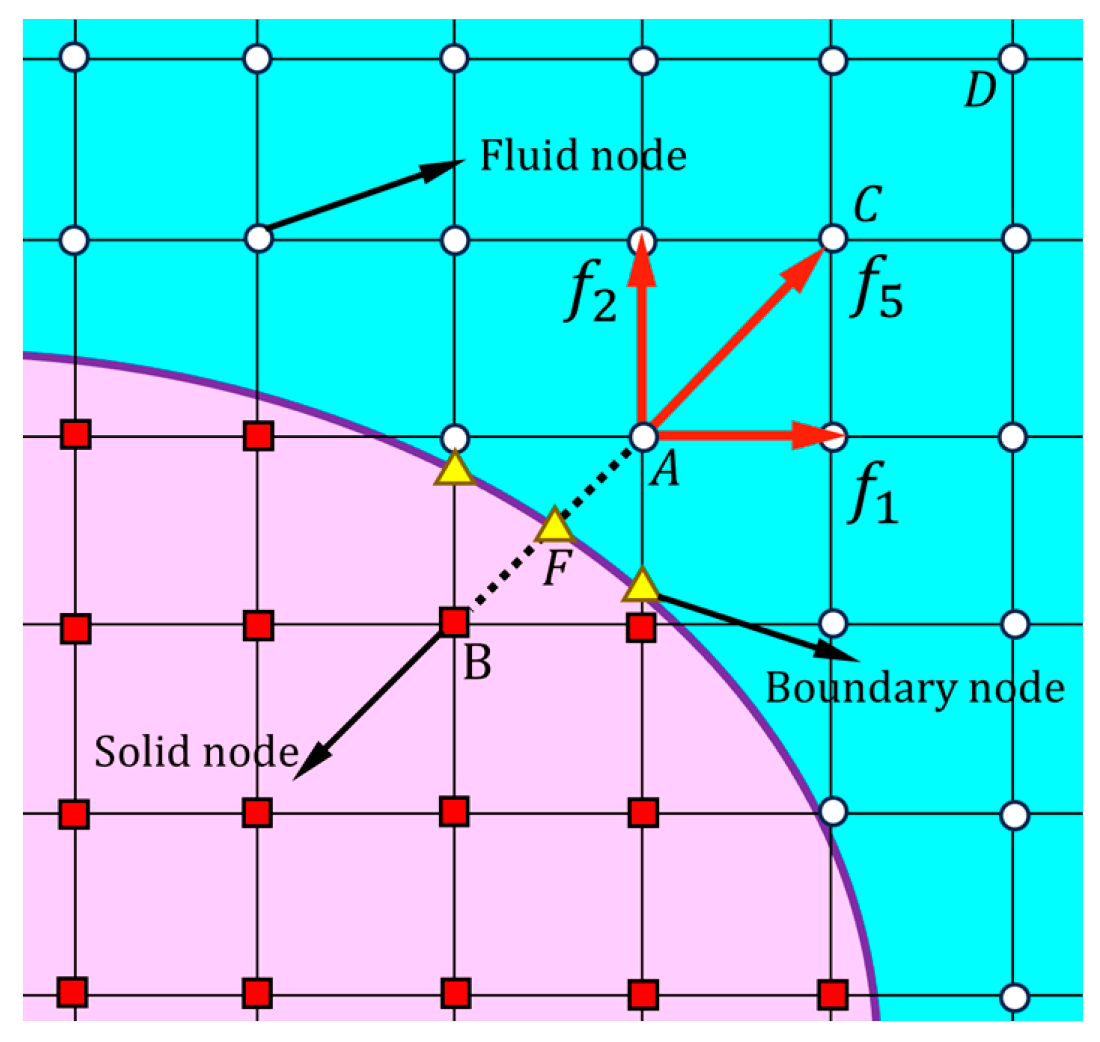
The non-slip boundary condition was adopted for both the wall and the two cylindrical surfaces. The non-slip boundary condition is a common boundary condition in fluid dynamics that requires the velocity of the fluid at the solid boundary to be zero. The no-slip boundary condition in the LBM is typically implemented using a bounce-back scheme. Specifically, when the fluid particles reach the solid boundary, they bounce back to their original lattice points, thus ensuring zero velocity at the boundary. In Fig. 3, the red square represents a solid node, and the white circle represents a fluid node. Considering node A as an example, the fluid-distribution function has three unknown values after the flow step, i.e., f 1 , f 2 and f 5 . To satisfy the no-slip boundary conditions on curved surfaces, the conventional bounce boundary scheme, that is, f 1 = f 3 , f 2 = f 4 , and f 5 = f 7 , can be adopted. To describe the bending boundary accurately, the parameter q is introduced, which is defined as the fraction of crosslinks that lie within the fluid region. For example, for node A, the value of q was determined to be q = A F / A B .
Taking the unknown fluid-distribution function f 5 of node A as an example, the calculation formula is as follows, according to different values of q : When q < 1 2 , f5A=q1+2qf7B+1−4q2f7A−q1−2qf7C−2w7ρfe7·uNcs2(11) where u N is the boundary node velocity ( u N = 0 under non-slip boundary condition), and f i X denotes the value of the distribution function at node X along direction i ; When q ≥ 1 2 ,
f5A=1q2q+1f7B+2q−1qf5C−2q−12q+1f5D−2w7ρfq2q+1e7·uNcs2(12) The remaining unknown distribution functions were determined using a similar method to ensure that the boundary conditions were accurately realized. After the boundary conditions were determined, the total force F exerted by the fluid on the cylinder was calculated using the momentum exchange scheme. According to the method of He & Doolen [25], the total force can be obtained by integrating the stress of ∂ Ω on a cylindrical surface: F=∫∂ΩdAn^·−pI+ρv∇:u+∇:uT(13) where n is the outer normal unit vector of the surface ∂ Ω , and I is the second-order unit tensor. The pressure can be obtained from the equation of state p = ρ c s 2 , where c s is the speed of sound.

Figure 3: Schematic of the bounce-back scheme in the LBM proposed by Lallemand & Luo [26]. Red squares represent solid nodes, white circles represent fluid nodes, and yellow triangles represent boundary nodes.
To better analyze the influence of the fluid on the cylinder, the drag coefficient C D and lift coefficient C L were introduced, which are defined as follows:
CD=FD0.5ρ U02D, CL=FL0.5ρ U02D(14) 3 Validation
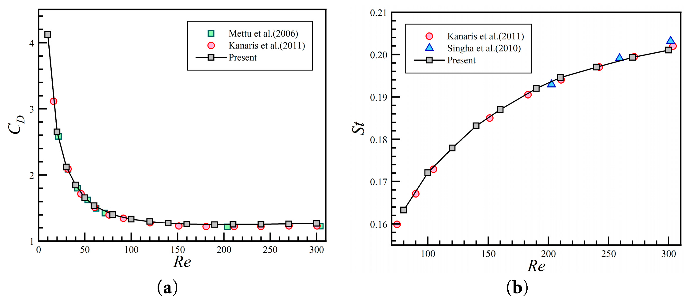
To verify the reliability of the calculated code, the flow around a single cylinder with a blocking ratio (defined as D / H ) β = 0.2 in a closed environment is simulated in the Reynolds number range of 10 to 300. The obtained drag coefficients C D were compared with the experimental results of Mettu et al. [27,28] (Fig. 4a), and Strouhal numbers S t were compared with the experimental results of Kanaris et al. [28,29] (Fig. 4b). Strong agreement is observed from the comparisons, indicating that the LBM is accurate and reliable.

Figure 4: Comparison of single cylinder winding simulation data with previous studies for the condition of blockage ratio β = 0.2 . (a) Drag coefficient C D [27,28]; and (b) Strouhal number S t [28,29].
4 Results
The flow was simulated for Reynolds numbers ranging from 0.1 to 160, assuming laminar and two-dimensional flow.
4.1 Steady Solutions
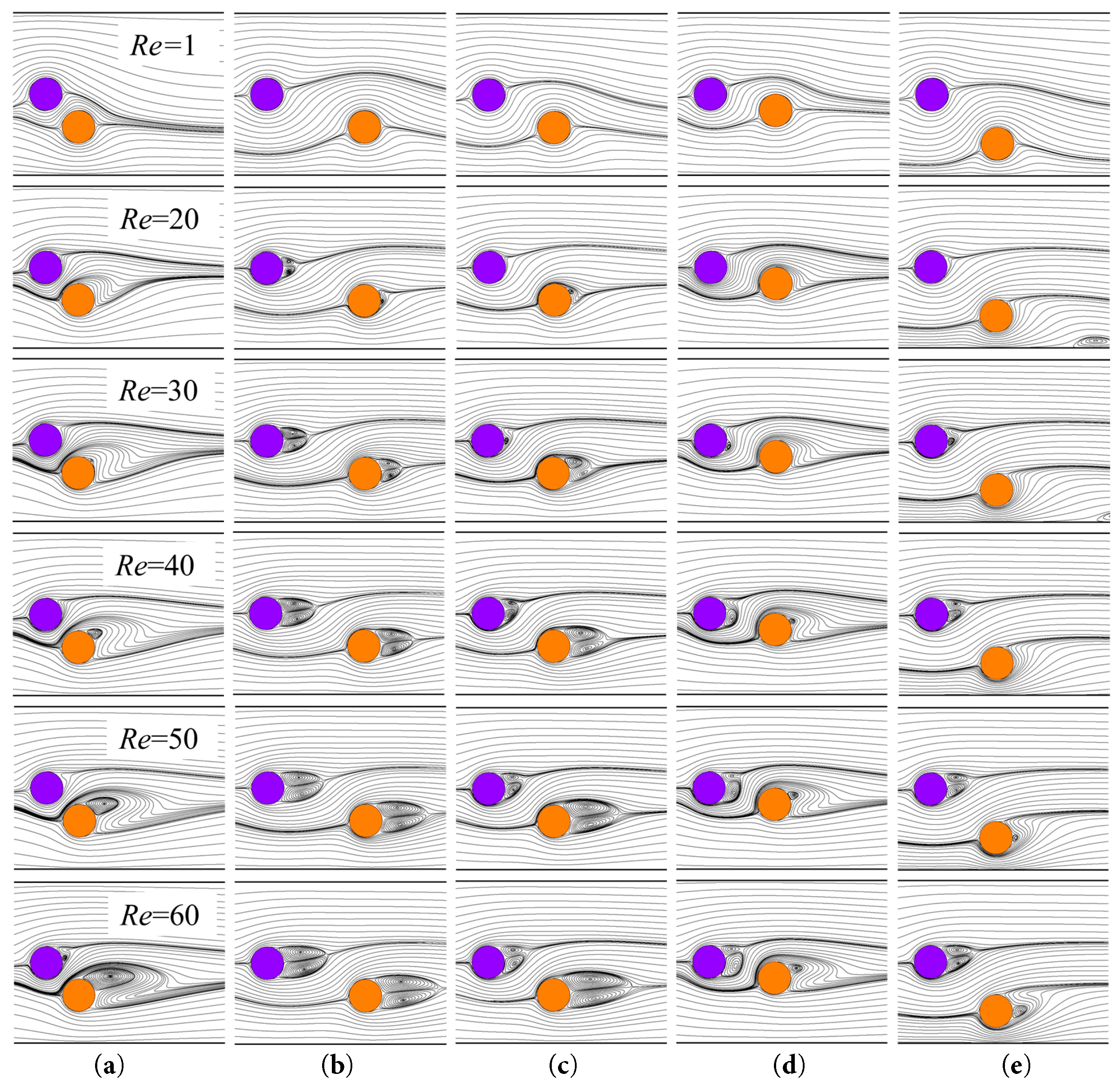
Steady-state flow was observed at a low Reynolds number. Reynolds numbers of 1, 20, 30, 40, 50, and 60 were selected as representative cases, and the streamline diagrams for these cases are shown in Fig. 5.

Figure 5: Streamline diagrams under low Reynolds number conditions for different cases: (a) Case 1; (b) Case 2; (c) Case 3; (d) Case 4; and (e) Case 5.
At R e = 1 , there is no flow separation due to viscous forces. With a gradual increase in the Reynolds number, flow separation occurs first in Case 2 (Fig. 5b), and then in Cases 3, 5, 4, and 1 (Fig. 5a,c–e).
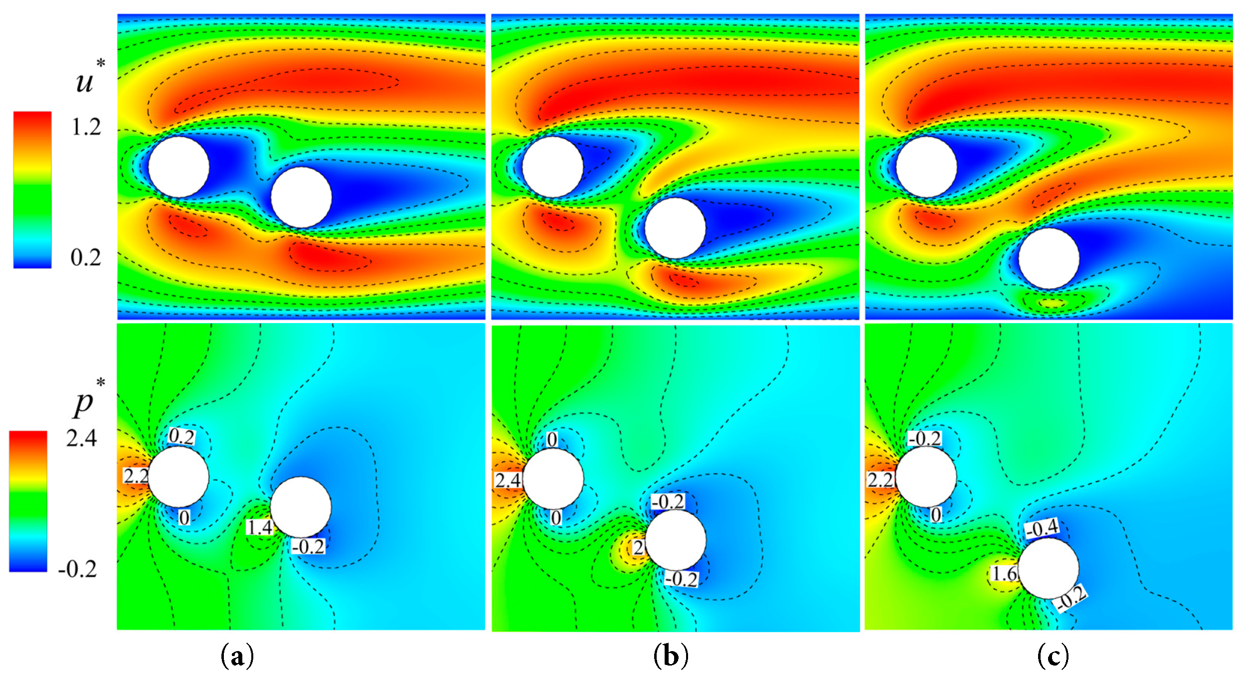
Decreasing the value of l significantly suppressed the flow separation phenomenon in cylinder 1 (Fig. 5a). The instantaneous velocity diagram in Fig. 6a shows that at small gaps between cylinder 1 and cylinder 2, the local acceleration zone on the lower side of cylinder 1 disappears and appears on the lower side of cylinder 2, making the two cylinders manifest as a whole in the flow field. The low-pressure zone in the middle of the two cylinders can also be found connected in the instantaneous pressure diagram in Fig. 6a. Additionally, the flow around cylinder 2 reduced the growth space of the recirculation zone of cylinder 1, causing the flow separation phenomenon of cylinder 1 to lag, and the recirculation zone to grow slowly. When the value of l is too large, the influence between the two cylinders is weakened, similar to the flow phenomenon around the two separate cylinders, whose flow separation occurs almost simultaneously, and the growth rate of the recirculation zone is almost the same (Fig. 5b). Fig. 6c shows that both cylinders form a pair of local acceleration zones, and the tail low-pressure zone also exhibits high independence.

Figure 6: Normalized instantaneous velocity and pressure at R e = 40 : (a) Case 1; (b) Case 3; and (c) Case 2. The normalized velocity formula is u * = u / U 0 . The normalization formula used is p * = p − p ∞ / 0.5 ρ U 0 2 . The value of p ∞ represents the freestream pressure.
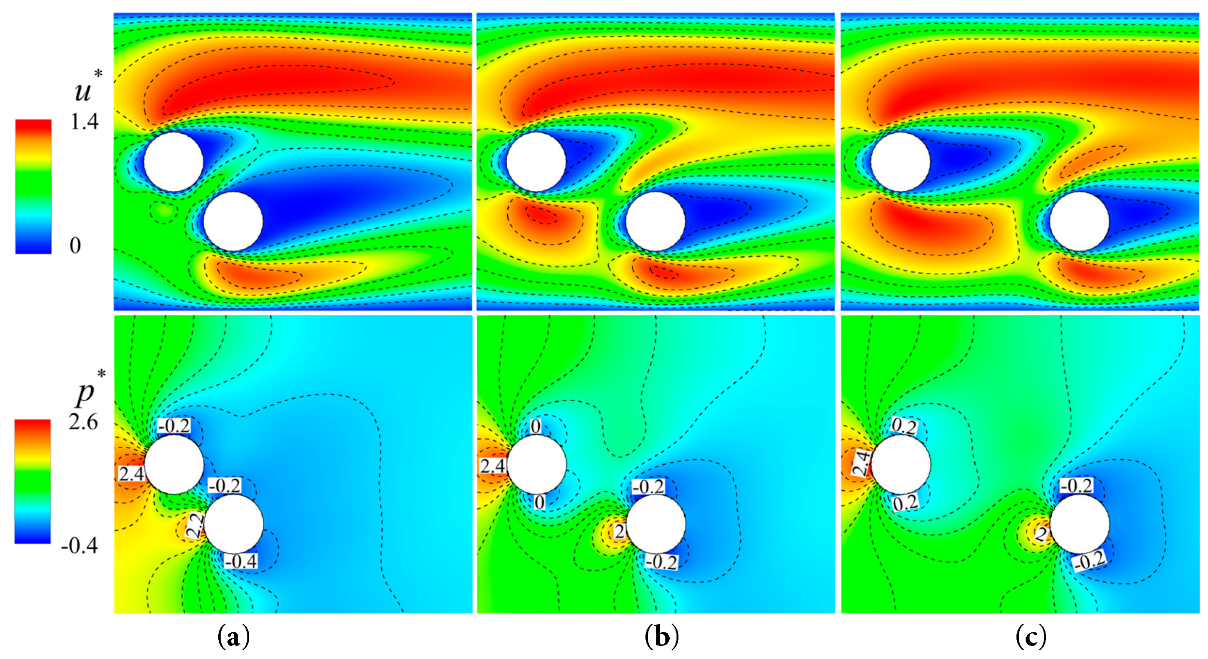
For Case 3, Case 4, and Case 5, the streamlines (Fig. 5c–e) show that changes in the value of h have a relatively small effect on both the magnitude of the critical Reynolds number at which the flow separation of cylinder 1 is generated and the growth rate of the recirculation zone. However, too small or too large value of h inhibits the flow separation of cylinder 2, which can be explained by the instantaneous velocities and pressures shown in Fig. 7. The flow around cylinder 1 forms a local acceleration zone, and cylinder 2 in Case 3 is affected by the localized acceleration zone, resulting in an increase in the surface pressure gradient and thus premature flow separation. However, when cylinder 2 is too close to or far away from cylinder 1 in the h direction, it will be less affected by the local acceleration zone. As shown in Fig. 7, the front-end pressure of cylinder 2 in Case 3 was significantly higher than that in the other two cases. Because cylinder 2 in Cases 4 and 5 is only affected by a localized acceleration zone on one side, there is only one low-pressure zone on the back, which explains why only one vortex is produced in the recirculation zone (Fig. 5d,e). The lower wall of Case 5 exhibited flow separation (Fig. 5e), which shifted back and weakened as the Reynolds number increased. This is because cylinder 2 is close to the lower wall, and its wake is close to the lower wall, resulting in a large velocity gradient and the generation of vorticity near the wall. With an increase in the Reynolds number, the wake of cylinder 2 gradually moved away from the lower wall.

Figure 7: Normalized instantaneous velocity and pressure at R e = 40 : (a) Case 4; (b) Case 3; and (c) Case 5. The normalized velocity formula is u * = u / U 0 . The normalization formula used is p * = p − p ∞ / 0.5 ρ U 0 2 . The value of p ∞ represents the freestream pressure.
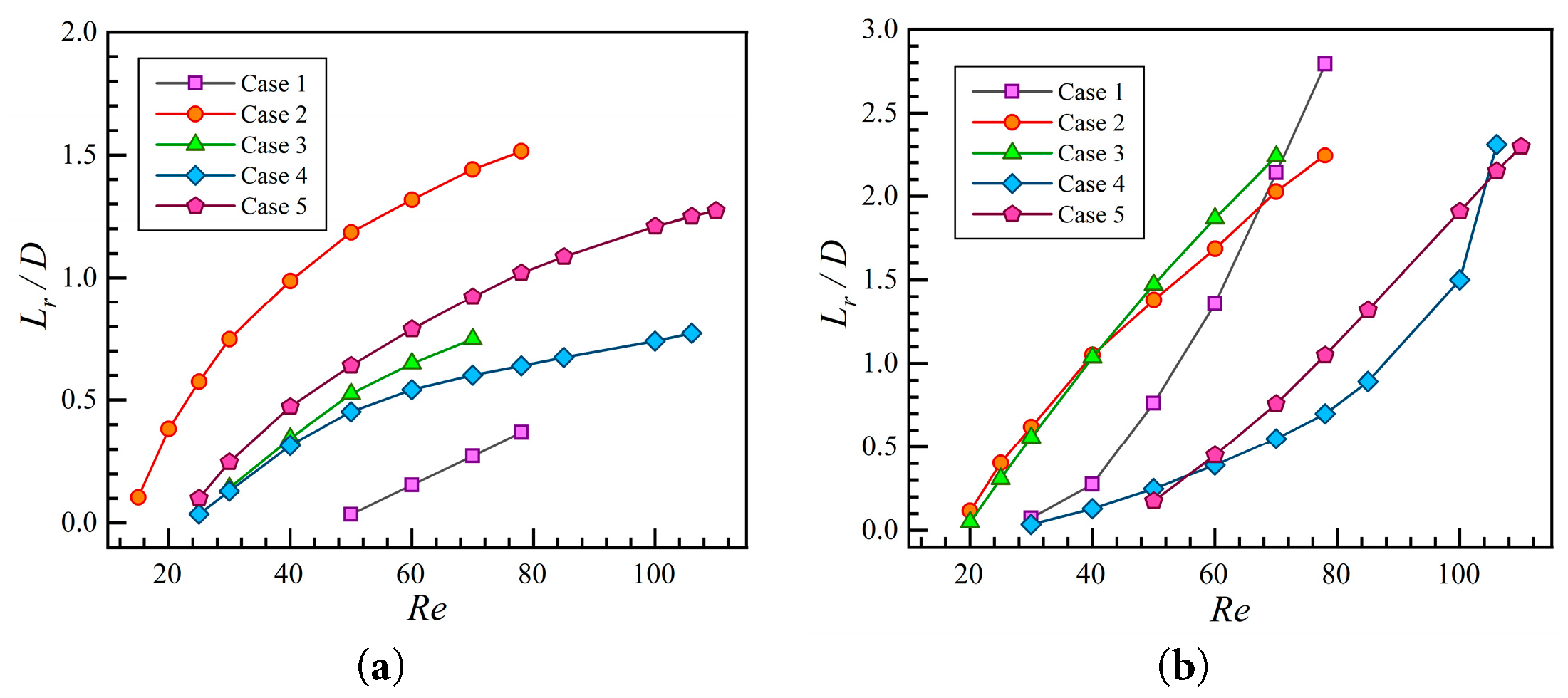
Additionally, the growth rate of the recirculation zone behind cylinder 2 was significantly greater than that behind cylinder 1, even in cases where the recirculation zone first appeared behind cylinder 1 (Fig. 8). The flow around cylinder 2 limits the growth of the recirculation zone of cylinder 1. Therefore, as the Reynolds number increases, the length of the recirculation zone of cylinder 1 increases, but the growth rate slows down. Fig. 8a shows that under a fixed Reynolds number, reducing l or h can reduce the length of the recirculation zone of cylinder 1, and the influence in the l direction is more obvious. Comparing Fig. 8a,b, the smaller the recirculation zone after cylinder 1 is suppressed, the faster the recirculation zone after cylinder 2 develops, and the longer the final length it reaches, which is consistent with the conservation of energy.

Figure 8: The recirculation length ( L r / D ) varies with the Reynolds number R e for all cases. (a) Cylinder 1 for all cases; and (b) Cylinder 2 for all cases.
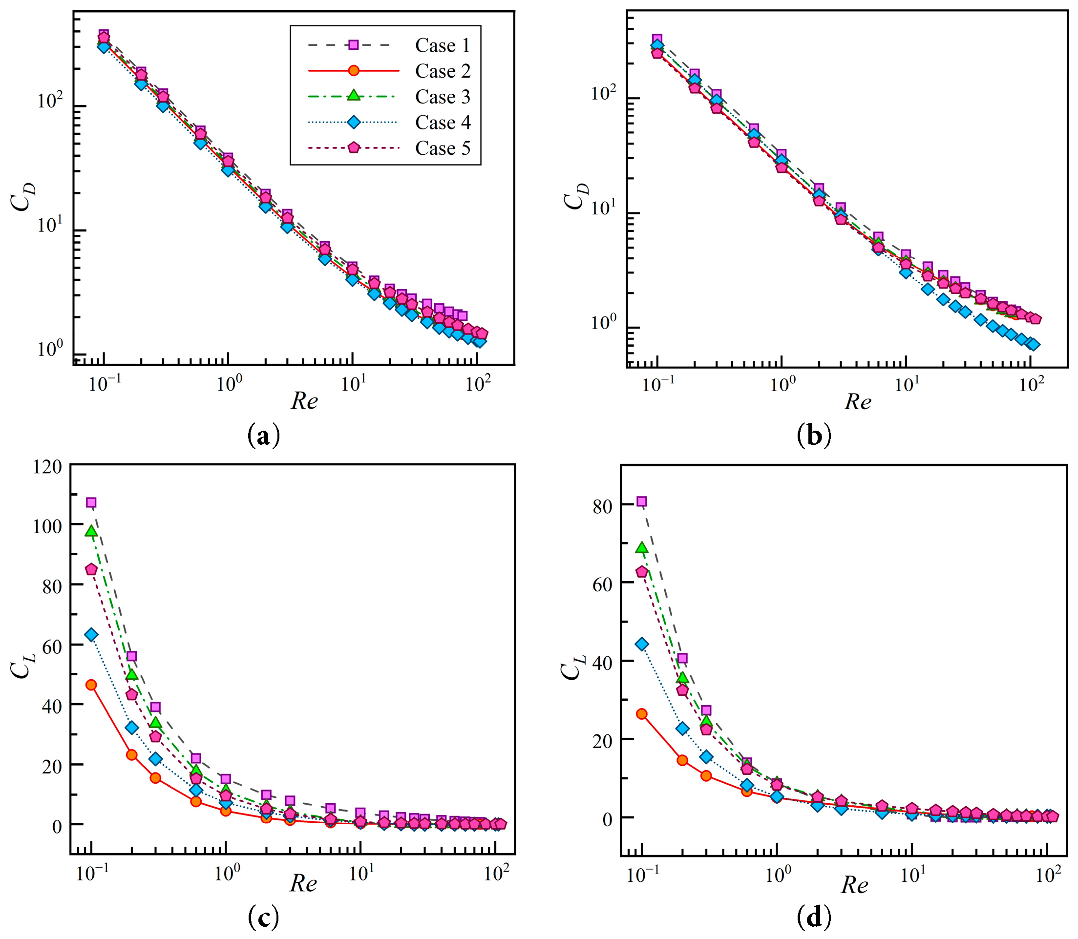
Fig. 9 shows that as the Reynolds number gradually increases, the C D and C L values of the two cylinders for all cases decrease sharply because of the interaction between friction (viscosity) and the pressure of the fluid on the cylinders as Re increases. For a fixed value of Re, the drag coefficient C D of Case 4, cylinder 2, exhibits the most significant decreasing trend, and at R e = 50 , it becomes the lowest of all cases. This gap continues to increase with the Reynolds number. It can be seen that the drag and lift coefficients of the two cylinders in Case 1 are almost the highest because the two cylinders in Case 1 are similar to a whole in the performance of the flow field, which makes this whole have a larger blockage ratio compared to the original, Fig. 6a shows that the high-pressure and low-pressure zones of the two cylinders in case1 are stronger than those of the other cases.

Figure 9: All cases in a steady flow state: (a) variation of the resistance coefficient C D of cylinder 1; (b) variation of the resistance coefficient C D of cylinder 2; (c) variation of the lift coefficient C L of cylinder 1; and (d) variation of the lift coefficient C L of cylinder 2.
4.2 Transition
With an increase in the Reynolds number, the flow begins to lose symmetry, a periodic vortex shedding phenomenon (Karman vortex street) occurs, and the flow state undergoes a fundamental transformation corresponding to the Reynolds number, which is called the critical Reynolds number R e c . The critical Reynolds number formed by the Karman vortex street in an unenclosed cylindrical flow is generally considered to be R e c ≈ 47 , a theoretical, critical value based on linear stability analysis and experimental observations. Subsequent studies have shown that the presence of a wall can inhibit the transition of the flow state, and the critical Reynolds number of a closed full cylinder is about 69 at a blockage ratio of β = 0.2 , which is much higher than that of an unclosed flow [5].
In this study, the critical Reynolds numbers are R e c 1 ≈ 79 for Case 1, R e c 2 ≈ 79 for Case 2, R e c 3 ≈ 71 for Case 3, R e c 4 ≈ 107 for Case 4, and R e c 5 ≈ 112 for Case 5. The critical Reynolds number was higher in all cases than that in the case of a single cylinder in the closed state, suggesting that the inclusion of a second cylinder had an inhibitory effect on the transition of the flow state. The critical Reynolds numbers for Cases 4 and 5 are significantly higher than those for the other cases, which is consistent with the fact that flow separation occurs the latest in these two cases, as discussed in the previous section.
4.3 Periodic Solutions
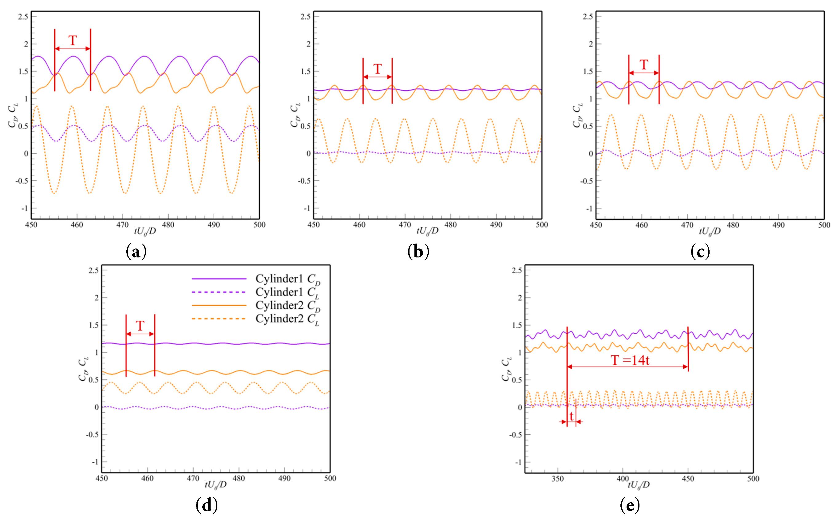
Fig. 10 shows the time evolution of the drag coefficient C D and lift coefficient C L for all cases of the two cylinders when the winding reached a steady periodic state for the R e = 160 condition. It can be found that the average drag coefficient C ¯ D of cylinder 1 is higher than that of cylinder 2 in all cases, and the C L fluctuation range of cylinder 2 is greater than that of cylinder 1. In particular, the C D of cylinder 2 in Case 1, Case 2, and Case 3 all exhibited sawtooth fluctuations to some extent. In Case 5, C D fluctuation is more complex, taking C L fluctuation as the small period t , C D fluctuation period T = 14 t , which is caused by the interaction between cylinder 2 near the wall and the wall standing vortex (discussed further below).

Figure 10: Time evolution of the coefficients of drag and lift for: (a) Case 1; (b) Case 2; (c) Case 3; (d) Case 4; and (e) Case 5 at R e = 160 when the flow reaches a periodic but statistical stationary state.
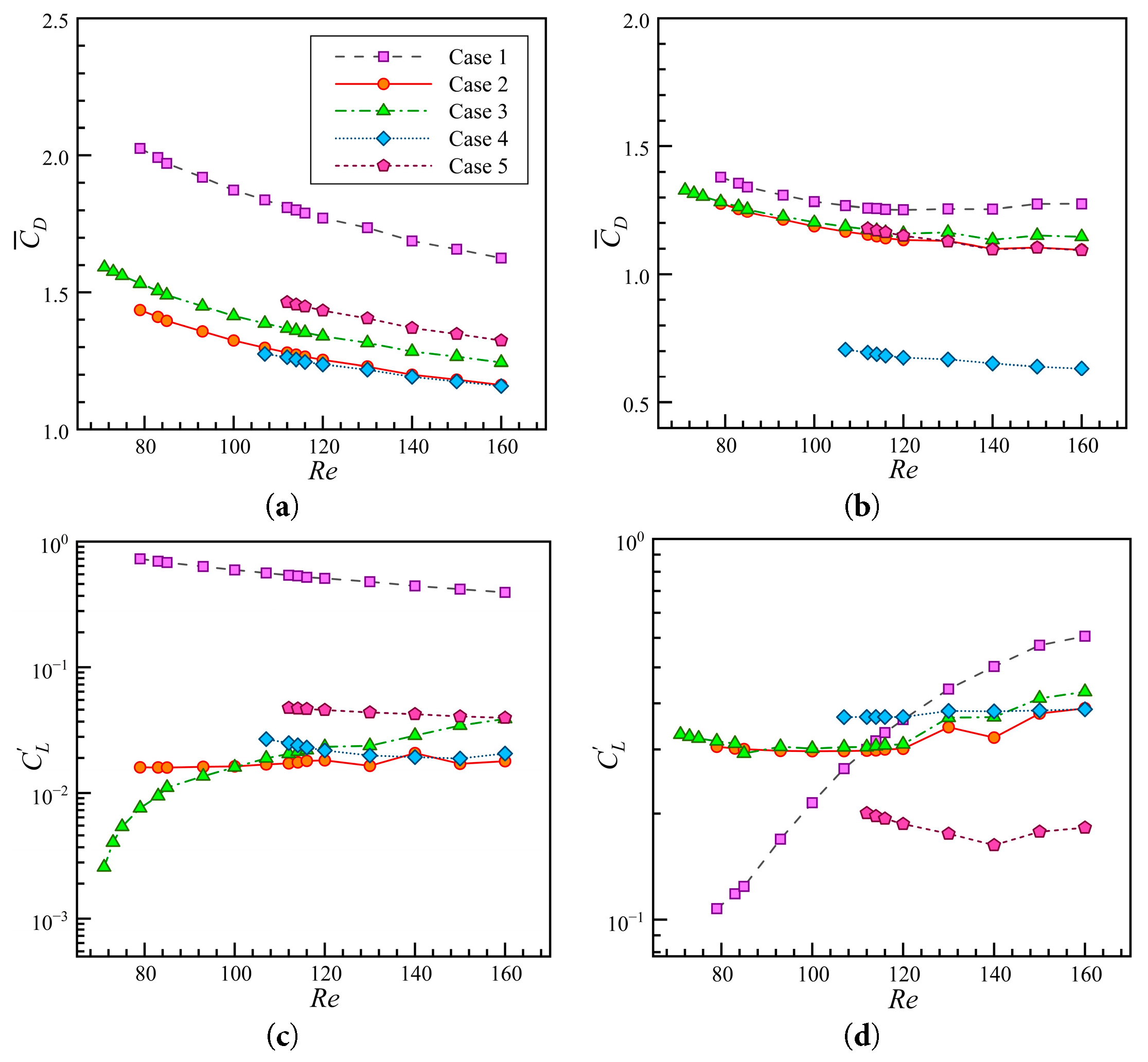
Fig. 11 illustrates the dependence of the mean drag coefficient C ¯ D and the root mean square of the lift coefficient C L ′ on the Reynolds number. As expected, the value of C ¯ D monotonically decreases with the Reynolds number (Fig. 11a,b). The decreasing trend of C ¯ D for the cylinders in all the cases was almost the same. C ¯ D for cylinder 1 in Case 1 was significantly higher than those in the other cases, and C ¯ D for cylinder 2 in Case 4 was significantly lower. The significant increase in C L ′ with increasing Reynolds number for Case 3 Cylinder 1 and Case 1 Cylinder 2 is because the vortex shedding strength at the rear of the cylinders increases significantly with increasing Re, increasing the instantaneous amplitude of lift. The significantly higher C ¯ D and C L ′ values for cylinder 1 in Case 1 suggest that a very small value of l significantly increases the flow oscillations produced by cylinder 1.

Figure 11: The relationship between (a) the average drag coefficient C ¯ D of cylinder 1; (b) the average drag coefficient C ¯ D of cylinder 2; (c) the root mean square of the lift coefficient C L ′ of cylinder 1; (d) the root mean square of the lift coefficient C L ′ of cylinder 2 and R e in all cases.
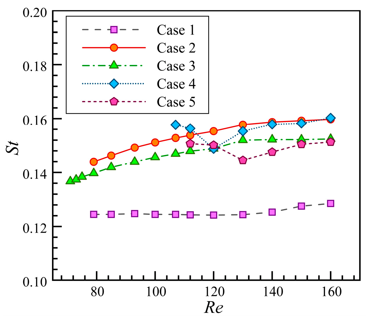
In all cases, S t eventually increased with Reynolds number (Fig. 12). The values of h and l for the five cases have a significant effect on its S t value. Decreasing l or increasing h reduces the frequency of vortex shedding, with the effect being more pronounced in the l direction.

Figure 12: Dependence of the Strouhal number S t of cylinder 2 on R e for the five cases.
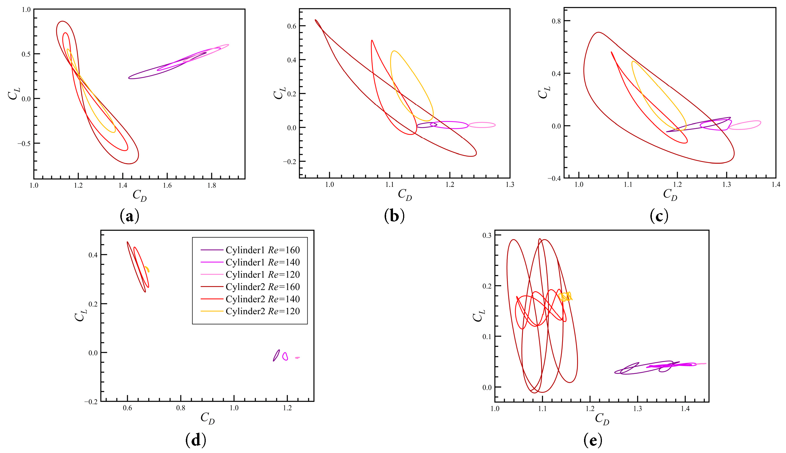
Phase diagrams were plotted based on the drag and lift coefficients for all the cases studied (Fig. 13). For a better visualization, only the results for Re = 120, 140, and 160 are shown. In all cases, the phase diagram gradually shifted to the left as the value of Re increased, which is consistent with the changes in C D (Fig. 11a,b). It can be observed that the amplitude of C L of cylinder 2 is greater than that of cylinder 1 in all cases, and the dependence of C L of cylinder 1 on Re is not obvious. The complexity of the phase diagram in Case 5 is related to complex fluctuations in C L .

Figure 13: Phase diagram constructed from C D and C L at different Reynolds numbers ( R e = 120, 140, and 160) for all the five cases. (a) Case 1; (b) Case 2; (c) Case 3; (d) Case 4; (e) Case 5.
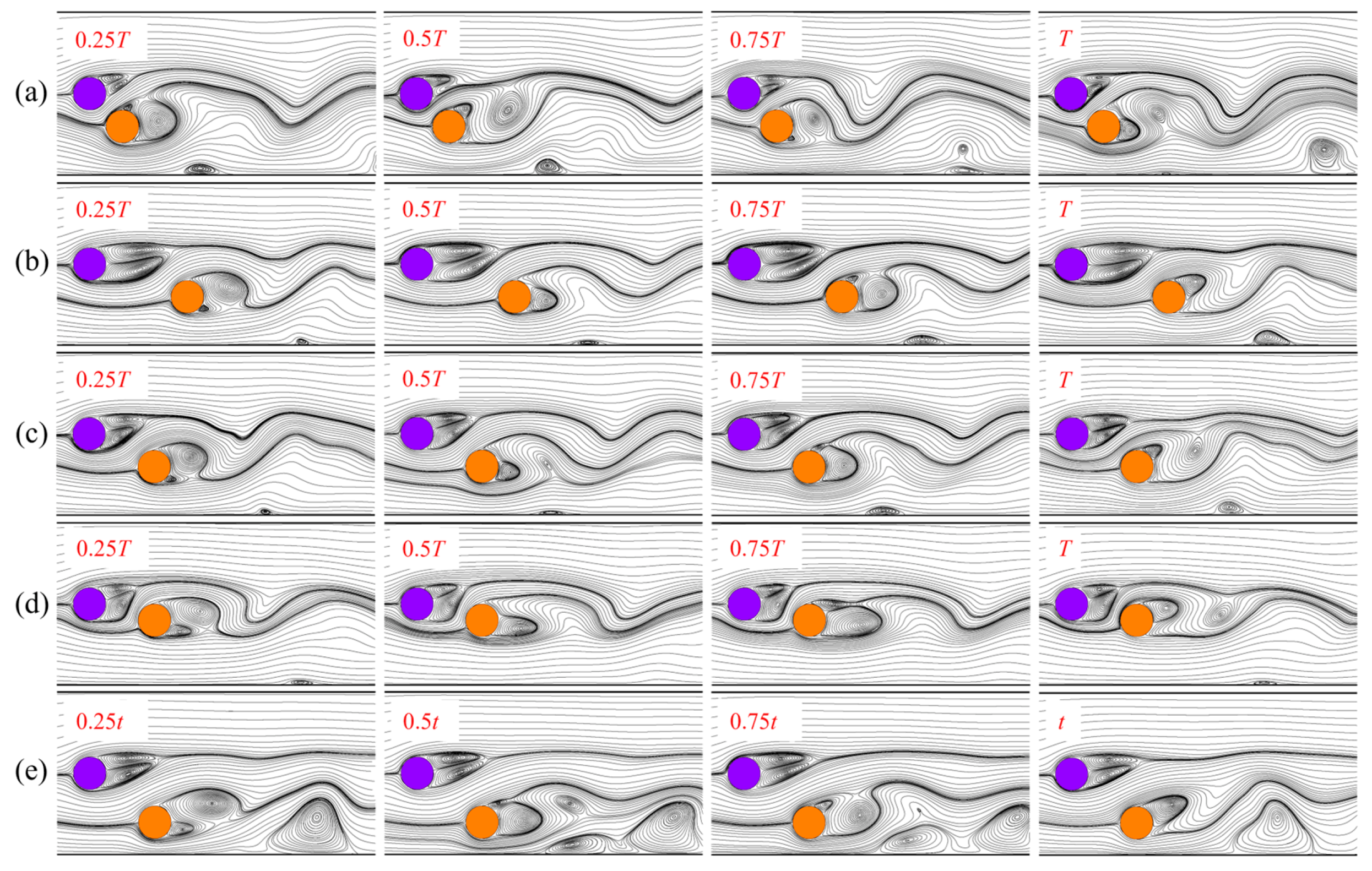
Fig. 14 illustrates the instantaneous streamline changes over one cycle for all cases (Case 5 is replaced by a small cycle t). In all cases, two vortices with opposite vorticities were observed to tumble alternately behind the cylinder, leading to periodic oscillations in the drag and lift of the cylinder. Vortex shedding mainly occurred in cylinder 2, which is why the amplitudes of C L in cylinder 2 were significantly larger than those in cylinder 1. Standing vortices were formed on the lower wall surface in all cases, with cylinder 2 in Case 5 resulting in larger and denser standing vortices on the wall owing to the close proximity of the wall and the significant influence of the rounding flow on the wall (Fig. 14e). These standing vortices merge with the shedding vortices and simultaneously affect the flow around the next small period t at the same time, resulting in complex fluctuations of cylinder 2 C D in Case 5.

Figure 14: Instantaneous streamlines at R e = 160 for the five cases during one period. (a) Case 1; (b) Case 2; (c) Case 3; (d) Case 4; (e) Case 5.
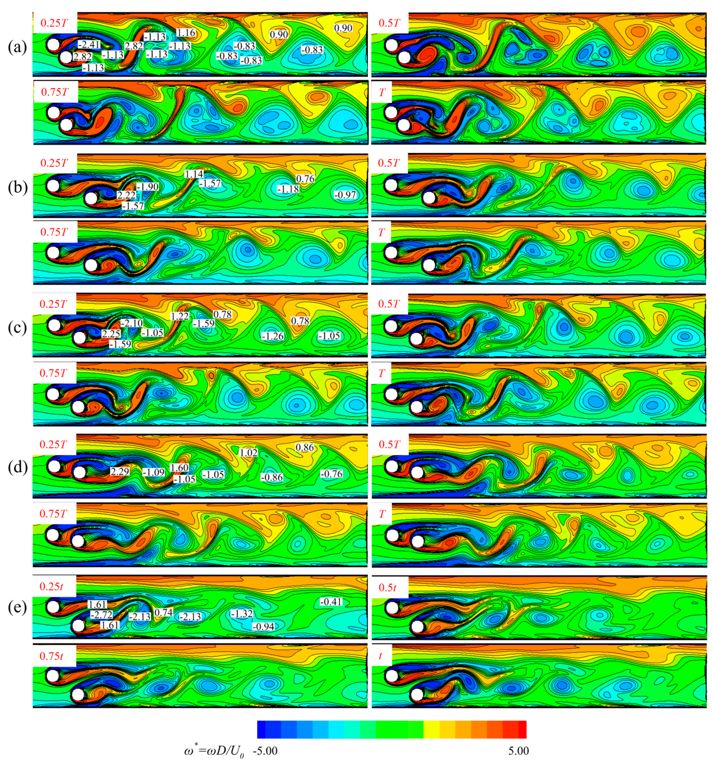
Fig. 15 shows the instantaneous vortex structure for one cycle at R e = 160 for the five cases. In all cases, the flow around the two cylinders formed positive and negative vorticities. The falling-off positive vorticity merged with the positive vorticity on the upper wall, and the negative vorticity on the lower wall peeled off and merged with the falling-off negative vorticity on the cylinder. A comparison of Cases 1, 2, and 3 reveals that decreasing l value leads to larger positive and negative vorticity downstream and larger downstream perturbation, and the negative vorticity shed by cylinder 1 weakens downstream as l increases (Fig. 15a–c). In particular, the negative vorticity shed by cylinders 1 and 2 and the lower wall surface of Case 1 are basically equal in magnitude, which leads to an equilibrium among the three vortices; instead of vortex merging, the three vortices form a whole that rotates while moving downstream in a short period of time. However, this structure caused the vortex to consume more energy, resulting in a significantly faster decay of the negative vorticity than in Cases 1 and 2 (Fig. 15a). Comparison of Case 3, Case 4, and Case 5 reveals that a decrease in h leads to a significant increase in the positive vorticity zone and a significant decrease in the negative vorticity zone (Fig. 15c–e). A comparison of Cases 3, 4, and 5 revealed that a decrease in h led to a significant increase in the positive vorticity region and a significant decrease in the negative vorticity region (Fig. 15c–e). This is because the negative vortex shedding of cylinder 2 is suppressed when h is small, owing to the influence of the tail flow of cylinder 1, whereas the positive vortex shedding of cylinder 2 is suppressed when h is large, owing to the influence of the wall. In Case 5, the negative vorticity presented a chaotic and complicated state mainly because the negative vorticity shed by cylinders 1 and 2 failed to merge, which also led to a rapid decay of the downstream negative vorticity (Fig. 15e).

Figure 15: Instantaneous vortices ( ω * = ω D / U 0 ) at R e = 160 for the five cases during one period. (a) Case 1; (b) Case 2; (c) Case 3; (d) Case 4; (e) Case 5.
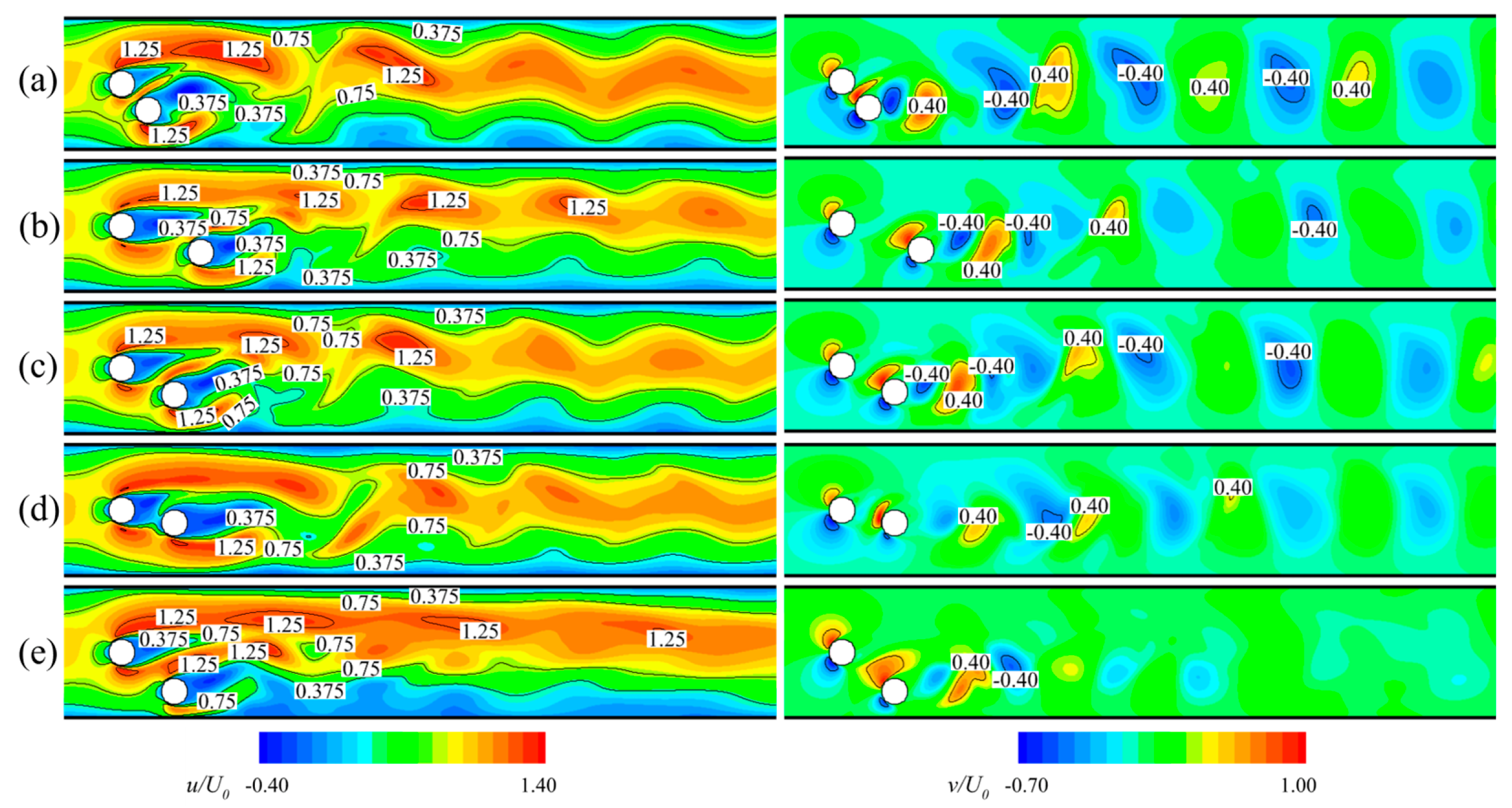
The study of the fluid velocity field can also shed light on the development of the wake behind a cylinder. Fig. 16 shows the instantaneous isograms of the streamwise velocity ( u / U 0 ) and normal velocity ( v / U 0 ) at R e = 160 for the five cases. Some representative values ( u / U 0 = 0.375, 0.75, and 1.125; v / U 0 = −0.4 and 0.4) are labeled for clarity of graphical representation. In all cases, the streamwise velocity at the center of the upper half of the region was greater than the entrance velocity U 0 . It was found that a decrease in l led to a more pronounced downstream disturbance, which is consistent with previous results (Fig. 16a–c). An increase in the value of h leads to a significant enhancement in the low-velocity region of the wall under the flow velocity (Fig. 16c–e). The normal perturbation downstream in Case 5 decays significantly faster than in the other scenarios, which is consistent with its vortex decay.

Figure 16: Streamwise component ( u / U 0 ) and normal component ( v / U 0 ) at R e = 160 for the five cases during one period. (a) Case 1; (b) Case 2; (c) Case 3; (d) Case 4; (e) Case 5.
5 Conclusions
The Poiseuille flow over two cylinders (designated as cylinders 1 and 2, respectively) confined between parallel walls was numerically studied for Reynolds numbers ranging between 0.1 and 160 (0.1 ≤ R e ≤ 160). Five particular cases were considered based on the vertical ( h ) and horizontal ( l ) distances between the two cylinders. Note that cylinder 1 was fixed at the central line while the position of cylinder 2 was varied. The summary of the findings is as follows.
- (1)A decrease in l significantly suppresses the flow separation of cylinder 1 at low Re, where the wake of the two cylinders is similar to that of a single bluff body. A small or large h inhibits the flow separation of cylinder 2, which is primarily due to the local acceleration zone formed by the wake of cylinder 1.
- (2)The critical Reynolds numbers were identified for the five cases, i.e., Rec1 ≈ 79, Rec2 ≈ 79, Rec3 ≈ 71, Rec4 ≈ 107, and Rec5 ≈ 112, each of which is higher than that of a single cylinder under the same conditions. This indicates that the hydrodynamic interaction between the cylinders harms the transition of the flow state.
- (3)It was shown that the forces on the cylinders vary periodically in connection with the vortex shedding at high Re. The average drag coefficient (C¯D) is larger for cylinder 1 than for cylinder 2 for all cases considered, and the oscillations in the lift coefficient (CL) are more significant for cylinder 2. Particularly, both the C¯D and the root mean square of the CL of cylinder 1 were noticeably larger for Case 1 (minimal l) compared with the other cases, suggesting that smaller vertical distances between the cylinders intensify the flow unsteadiness. The Strouhal number (St) increases with the Reynolds number for all cases. However, either of h and l has a significant effect on the variation in St. Specifically, decreasing l or increasing h reduces the frequency of vortex shedding.
References
1. Liang D, Cheng L, Li F. Numerical modeling of flow and scour below a pipeline in currents: part II. Scour simulation. Coast Eng. 2005;52(1):43–62. doi:10.1016/j.coastaleng.2004.09.001.
2. Zhu H, Qi X, Lin P, Yang Y. Numerical simulation of flow around a submarine pipe with a spoiler and current-induced scour beneath the pipe. Appl Ocean Res. 2013;41:87–100. doi:10.1016/j.apor.2013.03.005.
3. Kumar A, Dhiman A, Baranyi L. Fluid flow and heat transfer around a confined semi-circular cylinder: onset of vortex shedding and effects of Reynolds and Prandtl numbers. Int J Heat Mass Transf. 2016;102:417–25. doi:10.1016/j.ijheatmasstransfer.2016.06.026.
4. Chen WL, Huang Y, Chen C, Yu H, Gao D. Review of active control of circular cylinder flow. Ocean Eng. 2022;258:111840. doi:10.1016/j.oceaneng.2022.111840.
5. Sahin M, Owens RG. A numerical investigation of wall effects up to high blockage ratios on two-dimensional flow past a confined circular cylinder. Phys Fluids. 2004;16(5):1305–20. doi:10.1063/1.1668285.
6. Zhang W, Wang Y, Qian YH. Stability analysis for flow past a cylinder via lattice Boltzmann method and dynamic mode decomposition. Chin Phys B. 2015;24(6):064701. doi:10.1088/1674-1056/24/6/064701.
7. Nie D, Lin J. Numerical study on flow past a confined half cylinder in two bluff arrangements. Fluid Dyn Res. 2019;52(1):015506. doi:10.1088/1873-7005/ab5842.
8. Mashhadi A, Sohankar A, Alam MM. Flow over rectangular cylinder: effects of cylinder aspect ratio and Reynolds number. Int J Mech Sci. 2021;195:106264. doi:10.1016/j.ijmecsci.2020.106264.
9. Abdelhamid T, Alam MM, Islam M. Heat transfer and flow around cylinder: effect of corner radius and Reynolds number. Int J Heat Mass Transf. 2021;171:121105. doi:10.1016/j.ijheatmasstransfer.2021.121105.
10. Li J, Zhang M. Reinforcement-learning-based control of confined cylinder wakes with stability analyses. J Fluid Mech. 2022;932:A44. doi:10.1017/jfm.2021.1045.
11. Li S, Yang J, Teng P. Data-driven prediction of cylinder-induced unsteady wake flow. Appl Ocean Res. 2024;150:104114. doi:10.1016/j.apor.2024.104114.
12. Al-Sadawi LA, Mohammed AF, Biedermann TM, Yusaf T. The influence of a divergent slot on the near-wake region of a circular cylinder. Int J Thermofluids. 2024;24:100985. doi:10.1016/j.ijft.2024.100985.
13. Amini Y, Izadpanah E, Zeinali M. A comprehensive study on the power-law fluid flow around and through a porous cylinder with different aspect ratios. Ocean Eng. 2024;296:117035. doi:10.1016/j.oceaneng.2024.117035.
14. Ren F, Wang C, Song J, Tang H. Deep reinforcement learning finds a new strategy for vortex-induced vibration control. J Fluid Mech. 2024;990:A7. doi:10.1017/jfm.2024.503.
15. Alam MM, Zheng Q, Hourigan K. The wake and thrust by four side-by-side cylinders at a low Re. J Fluids Struct. 2017;70:131–44. doi:10.1016/j.jfluidstructs.2017.01.014.
16. Alam MM. Effects of mass and damping on flow-induced vibration of a cylinder interacting with the wake of another cylinder at high reduced velocities. Energies. 2021;14(16):5148. doi:10.3390/en14165148.
17. Ahmad S, Waqas H, Liu D, Muhammad T, Khan I, Eldin SM. Flow transition and fluid forces reduction for flow around two tandem cylinders. Results Phys. 2023;51:106681. doi:10.1016/j.rinp.2023.106681.
18. Kalsoom S, Abbasi WS, Manzoor R. Numerical study of flow past two square cylinders with horizontal detached control rod through passive control method. AIP Adv. 2024;14(6):065009. doi:10.1063/5.0208743.
19. Gul F, Nazeer G, Sana M, Shigri SH, Ul Islam S. Numerical investigation of flow features for two horizontal rectangular polygons. AIP Adv. 2024;14(1):015347. doi:10.1063/5.0186721.
20. Ali U, Islam M, Janajreh I, Fatt YY, Alam MM. Hydrodynamic and thermal behavior of tandem, staggered, and side-by-side dual cylinders. Phys Fluids. 2024;36(1):013605. doi:10.1063/5.0176710.
21. Yu D, Mei R, Luo LS, Shyy W. Viscous flow computations with the method of lattice Boltzmann equation. Prog Aerosp Sci. 2003;39(5):329–67. doi:10.1016/S0376-0421(03)00003-4.
22. Bhatnagar PL, Gross EP, Krook M. A model for collision processes in gases. I. Small amplitude processes in charged and neutral one-component systems. Phys Rev. 1954;94(3):511. doi:10.1103/PhysRev.94.511.
23. He X, Luo LS. A priori derivation of the lattice Boltzmann equation. Phys Rev E. 1997;55(6):R6333. doi:10.1103/PhysRevE.55.R6333.
24. Qian YH, d’Humières D, Lallemand P. Lattice BGK models for Navier-Stokes equation. Europhys Lett. 1992;17(6):479. doi:10.1209/0295-5075/17/6/001.
25. He X, Doolen G. Lattice Boltzmann method on curvilinear coordinates system: flow around a circular cylinder. J Comput Phys. 1997;134(2):306–15. doi:10.1006/jcph.1997.5709.
26. Lallemand P, Luo LS. Lattice Boltzmann method for moving boundaries. J Comput Phys. 2003;184(2):406–21. doi:10.1016/S0021-9991(02)00022-0.
27. Mettu S, Verma N, Chhabra RP. Momentum and heat transfer from an asymmetrically confined circular cylinder in a plane channel. Heat Mass Transf. 2006;42(11):1037–48. doi:10.1007/s00231-005-0074-6.
28. Kanaris N, Grigoriadis D, Kassinos S. Three dimensional flow around a circular cylinder confined in a plane channel. Phys Fluids. 2011;23(6):064106. doi:10.1063/1.3599703.
29. Singha S, Sinhamahapatra KP. Flow past a circular cylinder between parallel walls at low Reynolds numbers. Ocean Eng. 2010;37(8–9):757–69. doi:10.1016/j.oceaneng.2010.02.012.

 Submit a Paper
 Propose a Special lssue
 Open Access
 View Full Text
 Download PDF
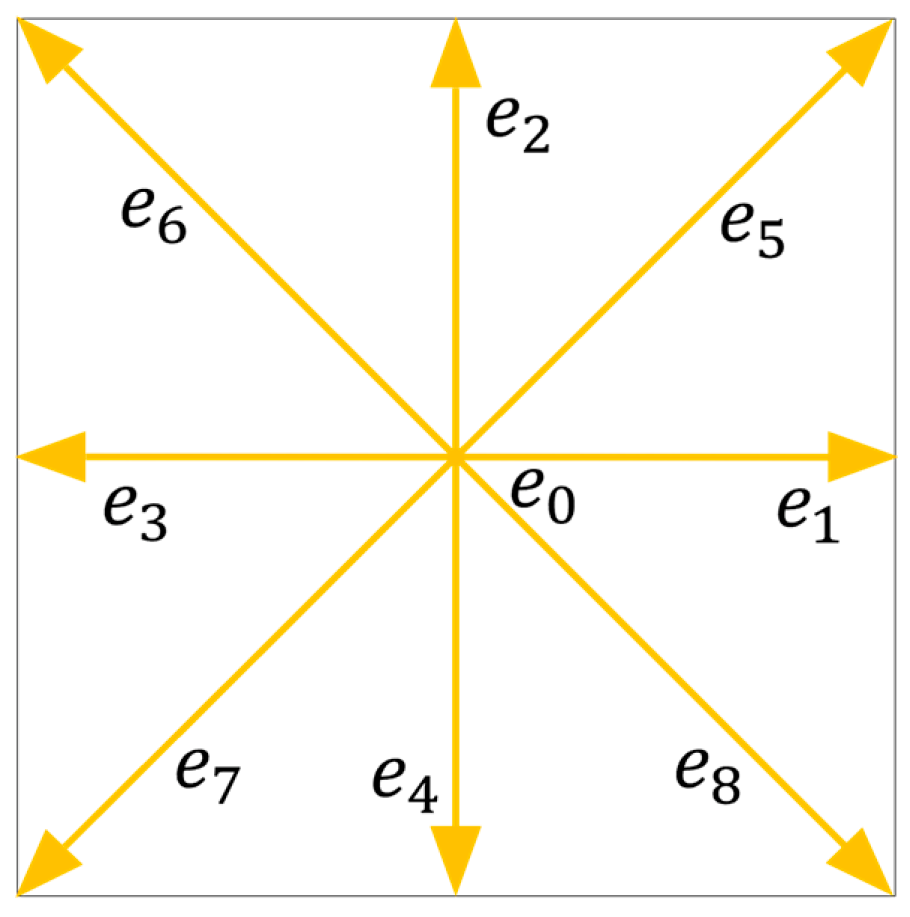
 Copyright © 2025 The Author(s). Published by Tech Science Press.
 Downloads
 Citation Tools