Temperature-Difference Driven Aggregation of Pulling- and Pushing-Typed Microswimmers in a Channel

1 Introduction

With the exploration of the microscopic world, the study of microswimmers has been widely emphasized in recent decades. These swimmers have immense potential in diverse applications such as water purification [1], robotics [2], and biomedicine [3]. Unlike passive particles, microswimmers possess the unique capability to harness energy from their environment [4], including chemical, light, and electrical sources. To emulate these mobilizers, most research models have been derived from naturally occurring microorganisms such as bacteria and algae. Different species of microorganisms exhibit different community behavior [5]. Notably, when immersed in a fluid, the microswimmers are inevitably susceptible to Brownian motion. Specifically, previous studies determined a strong correlation between the Brownian motion of these microswimmers and ambient temperature [6,7]. Based on this, people have conducted varying degrees of research on different particles and Brownian motion.

To study the motion of microswimmers in complex environments, researchers have conducted a series of studies based on the squirmer model, which is a microbial-based peristaltic model proposed by Lighthill [8] and modified by Blake [9]. The model can effectively solve the problem of simulating microbial models with different propulsion modes and shapes. Based on this model, people have conducted thorough research on the dynamic characteristics of individual particles, different shapes and multiple particles, respectively. More and Ardekani [10] examined the motion of a squirmer in a density-stratified fluid using a direct numerical simulation. The stability of the motion of the puller and pusher in different stratifications exhibited a large difference. Ouyang and Lin [11] simulated the settling of a single squirmer in a narrow channel and identified four typical motion modes: vertical, attracted, oscillatory, and upward. Density ratio and inertia were also found to significantly influence these modes. Ishimoto et al. [12] simulated the kinetic behavior of a squirmer on a periodic sinusoidal interface and analyzed how the squirmer was guided by surfaces with different morphologies. Zheng et al. [13] simulated the motion of a squirmer near curved obstacles and investigated the use of a puller and pusher to guide the motion of the squirmer. We investigated how the motion patterns of the puller and pusher changed after collisions with obstacles. The results revealed six swimming modes of the squirmer: dancing forward, C-loop, orbiting forward, ∞-loop, scattering, and orbiting backward.

In addition to studying circular and spherical particles, studies investigated rod and ellipsoidal particles, which are closer to the actual shape. Zantop and Stark [14] simulated the dynamics of long rod-like squirmer particles stacked by multiple circular squirmer arrangements during the motion of the shape structure, and they discussed the composition of the hydrodynamic moments in the flow field of three different types of rod-like squirmers. Ouyang and Lin [15] used the immersed boundary-lattice Boltzmann method to simulate the motion of elongated rod-like squirmer particles in a flow field and investigated their dynamic behavior. In the study, the hydrodynamic efficiency, swimming speed, and power consumption of the puller and pusher varied under different conditions. Liu et al. [16] used direct numerical simulations of elliptical squirmer motion in Poiseuille flow and found five typical modes of motion: periodic tumbling, chaotic migrating modes, stable sliding, unstable states, damped swinging, and three rheotaxis states: stable, substable, and unstable states. Additionally, a series of studies examined the complex movements between two or more microswimmers. Ishikawa et al. [17,18] successively numerically simulated the interactions between two microswimmers under different flow field conditions. In the simulation at low Reynolds number, it was determined that the two microswimmers were first attracted to each other during motion, then changed direction after contact, and finally separated. In the Stokes flow field of an infinite fluid, where the microswimmers were either bacteria with flagella or spherical bacteria, it was observed that the two bacteria avoided each other by changing their direction when approaching each other. Ziegler et al. [19] simulated the interaction of two three-sphere swimmers in a fluid by connecting three spheres into a single unit through a spring link to form a three-sphere swimmer. The results indicated that two three-sphere swimmers showed a significant increase in speed when compared to a single microswimmer and there were significant changes in the rotation and translation of the swimmers. Cavaiola [20] used direct numerical simulations to model the group motion of a slender puller and pusher at finite Reynolds numbers. The study analyzed the effect of inertia on microswimmers as well as the temporal and directional dependence of group motion. It was determined that the resulting complex dynamic behavior was closely related to the variation in Reynolds number. Ying et al. [21] simulated the settling pattern of two squirmers in a channel and found five typical patterns of motion: stable settling in the center, stable motion near the wall, wall attraction, oscillation, large oscillation, and small oscillation. Oscillations, large- and small-amplitude oscillations. Scholars have conducted thorough research on the dynamic characteristics of micro-moving devices based on the squirmer model.

Brownian motion of particles is important for particle applications and academic research. Microswimmers in fluid media are inevitably affected by Brownian motion. So that they play a significant role in the study of microswimmers. The discovery of Brownian motion in the nineteenth century was explored in studies through experiments, simulations, and theory. Iwashita and Yamamoto [22] and Drossinos and Reeks [23] simulated the short- and long-term motions of Brownian particles in a shear flow using a direct numerical simulation method. It was observed that the inertia of the fluid is important in short-term Brownian motion and that the diffusion coefficient of long-term Brownian particles exhibits a higher correlation with the inertia of the particles. Kümmel et al. [24] designed artificially active Brownian particles and observed an almost circular trajectory. This also indicates that ideal linear swimming is difficult to achieve in practical situations and that active particles whose equilibrium stability is broken under the effect of Brownian motion sometimes are chiral. Zöttl and Stark [25] examined the collective behavior of active Brownian particles, experimentally observed the dynamic properties of the particle population, and proposed a physical method to quantify the collective behavior of particles. Löwen [26] summarized a series of recent developments in active Brownian particles with inertia, including collective motion properties of single and multiple particles with inertia. Zanovello et al. [27] investigated the directional motion of active Brownian particles and observed that the success of active Brownian particles in reaching their targets can be improved via tuning their activity and persistence of active Brownian particles. Chen and Thiffeault [28] simulated different shapes of Brownian microswimmers in a channel, derived simplified equations for microswimmers in an infinite channel, disregarded fluid interactions, and analyzed the change in the swimming direction of two-dimensional active Brownian particles with a fixed velocity under the effect of Brownian motion. In addition, expressions for the time required for the miniature swimmer to completely change direction in the channel and the diffusion efficiency were calculated. Di Trapani et al. [29] examined active Brownian particles in a disk with an absorbing boundary, set up passive Brownian particles as the ground state and treated activeness as a perturbation. The corresponding time-dependent Fokker-Planck equation for active Brownian particles was solved, and the effects of the time and initial conditions on the accuracy of the solution were demonstrated.

It is well-known that the motion of Brownian particles is affected by the temperature of their surrounding environment. The aggregation and migration motion of Brownian particles due to temperature differences is known as the Ludwig–Soret effect, a phenomenon in which objects migrate due to temperature gradients. Kreft and Chen [30] indicated that this is due to the non-equilibrium stresses in the fluid induced by temperature gradients and that the effect is important in the study of diffusion in polymers and colloids. Dhlamini et al. [31] investigated the boundary layer flow of a stabilized nanofluid and discussed the effect of the Brownian and thermophoretic motions of particles on the irreversibility of heat transfer. It was demonstrated that heat generation enhanced the irreversibility of heat transfer. In their study on the thermal conductivity of nanocolloids, Prasher et al. [32] verified that convection induced by Brownian motion was the main reason for the enhanced thermal conductivity of these colloids. Zhu et al. [33] investigated the separation of mixtures of active and passive Brownian particles driven by temperature differences and updated the motions of the particles by solving the Langevin equation. The results indicated that it is possible to tune the motions of the active Brownian particles to change the direction of the motions through the temperature difference, whereas the motions of the passive particles are different. The difference is utilized to achieve the separation of the two types of particles. Michaelides [34] investigated the effect of a steady temperature gradient on the Brownian motion and thermophoresis of nanoparticles in liquids. The results suggested that the thermophoresis speed of the highly conductive nanoparticles was directly proportional to the kinematic viscosity of the fluid and the applied temperature gradient. Saghir and Mohamed [35] simulated thermal conduction in nanofluids by combining the Brownian motion and thermophoresis effects to analyze the effects of Brownian motion and thermophoresis on thermal conduction under different conditions. The results indicated that the effects of Brownian motion and thermophoresis can be neglected in a few cases. Uma et al. [36] investigated the interaction between Brownian motion and the hydrodynamics of nanoparticles in a flow field. The Brownian motion of nanoparticles in incompressible Newtonian fluids (stationary or fully developed Poiseuille flows) was investigated via the fluctuating hydrodynamic method. Nie and Lin [37] proposed the Fluctuating-Lattice Boltzmann Method (FLBM) for the direct numerical simulation of the Brownian motion of particles and constructed a three-dimensional FLBM model. Thus, Nie and Lin [38] investigated the aggregation effect of particles driven by the temperature difference in the channel based on the direct numerical simulation method of the FLBM, and added a heat transfer term that affects the temperature difference to make the simulation more reliable. The key factors affecting the performance and efficiency of temperature-driven particle aggregation were analyzed.

In previous research on the Brownian motion of self-propelled particles, simple active Brownian particles were mostly used as the model. The interactions between the particles were often neglected in the simulation process, and a large distance existed between the simulation and the real situation. There are still many gaps in the study of the population behavior of microbial particles under the influence of Brownian motion. Therefore, the present study used Lattice Boltzmann Method simulations to restore the interactions between the particles, and the motion of the fluid was coupled to the particle motion through the bounce-back scheme [39]. The particle-particle and the particle-wall collision problems were solved using the repulsive force model proposed by Glowinski et al. [40]. In addition, the microswimmers used in the study were constructed based on the squirmer model [9], which can realistically restore the motion of microorganisms in the flow field. We use the FLBM by Nie and Lin [37], the thermal fluctuations of fluid molecules were simulated by adding a stochastic stress tensor to the Lattice Boltzmann equations, and the motion of Brownian particles was modeled via solving the lattice Boltzmann equations and Newton’s equations, which simplified the calculations by eliminating the need to add a stochastic term to Newton’s equations. The study focused on simulating the aggregation behavior of a swarm of squirmer-model Brownian particles in a channel. Several crucial factors were considered during the analysis, including the influence of the driving characteristics of the squirmer particles, the effect of their self-propelling strength, the effect of the strength of the temperature difference, and the contribution of thermal diffusion within the fluid. In particular, both the Prandtl and Lewis numbers, which represent heat and momentum transfer, were included in the analysis.

The remainder of the study is organized as follows: In Section 2, the numerical method of the FLBM and squirmer model was used, and the collision model, heat transfer model, and important parameters are presented. In Section 3, the accuracy of the numerical method and model construction is verified. Section 4 discusses the aggregation efficiency and performance of the pullers and pushers under the effect of different variables. Finally, the results are summarized in Section 5.

2 Model and Method

2.1 Squirmer Model

Many near-cylindrical microorganisms exist in the biological world including Paramecia and Volvox. The microorganisms propel themselves by moving oscillating cilia on their cell surfaces. In order to simulate the motion characteristics of micro-mobile devices more realistically. This paper adopts the squirmer swimming model that mimics microorganisms [8,9]. Given the excellent symmetry of cylinders, biomorphic models are commonly simplified into two-dimensional planar circles. By decomposing ciliary vibrations into radial and tangential motions along a circular boundary, a two-dimensional self-propelled particle model can be established.

Fig. 1 shows the simplified geometry of the two-dimensional squirmer model moving to the right. The solutions for the radial and tangential velocity components in the Newton–Stokes fluid for the two-dimensional squirmer model are as follows [9]: vr00r0=a=∑n=0∞An0tcosnθ,vθ00r0=a=∑n=0∞Bn0tsinnθ(1) where r0 denotes the distance from any point on to the center of the squirmer, and θ denotes the angle between the swimming direction and the polar axis. An0 and Bn0 denote time-dependent amplitudes. Given the requirement that the net hydrodynamic force equals zero for a squirmer with steady swimming, the stable swimming velocity of the squirmer is Us = (B10 − A10)/2, where A10 = 0.

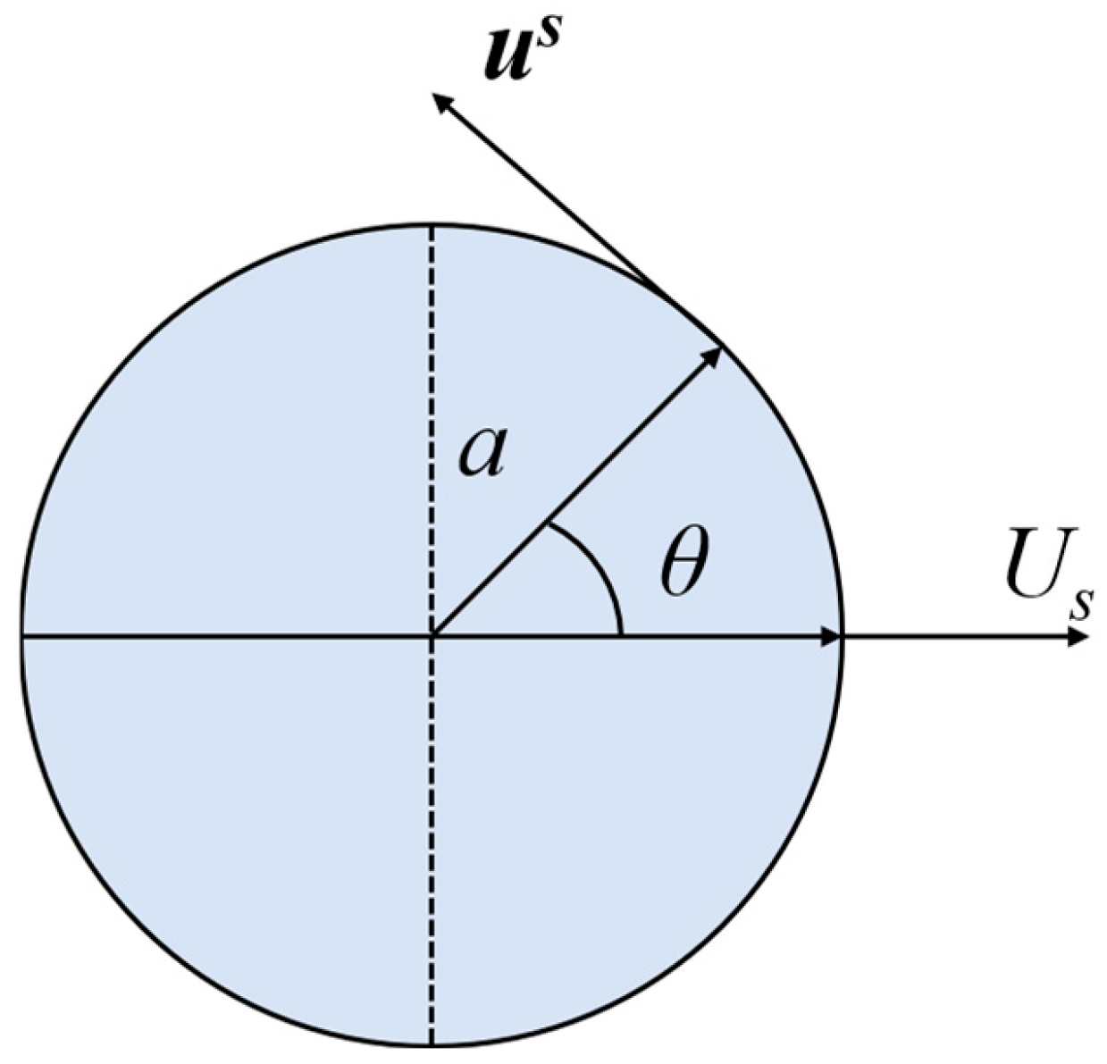
Figure 1: Two-dimensional schematic of a circular squirmer moving to the right.

The application of the model usually only considers tangential oscillations and neglects the effect of radial oscillations to simplify the model further. Hence, we can derive the reduced-order two-dimensional squirmer (n ≤ 2) with only the tangential boundary velocity:

The first term on the right side of the equation determines the stable swimming velocity Us = B1/2, representing a potential dipole with an irrotational singularity whose velocity decays with 1/r2. The second term represents a higher-order singular stress source that decays at 1/r in the flow field, resulting in vorticity around the squirmer. It should be noted that neither of these terms displayed an external effect on the squirmers. It is well known how fast decays the flow generated by a squirmer in three-dimensional, however, the two-dimensional result is not so well known.

Based on the driving mode, squirmers are primarily categorized into three types: pushers, pullers, and neutral. The parameter β = B2/B1 (B1 > 0) is defined and the value of β is used to indicate the different squirmer models (neutral is β = 0, puller is β > 0, and pusher is β < 0). A puller is a squirmer that moves by oscillating the cilia on its head, creating a pull forward to drag its motion such as a ciliate. A pusher is a squirmer that moves by oscillating the cilia on its tail and creates thrust forward to propel its motion in a manner similar to that of a flagellate. The model is based on the Stokes equation and its utility has been extended to intervals of moderate numerical Reynolds numbers.

2.2 Collision Model

This paper used a collision model to solve the collision problem of multiple particles. The elastic-force model was proposed by Glowinski et al. [40] is used to calculate the particle-particle and particle-wall collisions. The repulsive force for particle-particle collisions is defined as: Fijp=0cijεpRi+Rj+ξ−Sijξ2Xi−XjSijififSij>Ri+Rj+ξ,Sij≤Ri+Rj+ξ,(3) Ri and Rj denote the radii of the ith and jth particles, respectively, and Xi and Xj denote the coordinates of the centers of mass of the particles. Sij = |Xi − Xj| denotes the distance between the centers of mass of the two particles. ξ denotes the range of the repulsive force, which is set to 1.5Δx in the present simulation. εp denotes a stiffness parameter for the collision between the particles, which is set to 0.001 in the study, and cij is a scaling factor fixed at one. The repulsive force for particle-wall collisions is given by: Fijw=0cijεwRi+Rj+ξ−Sij ′ξ2Xi−Xj′ Sij′ if Sij ′>Ri+Rj+ξ,if Sij ′≤Ri+Rj+ξ,(4) Xj′ denotes the coordinate vector of the center of the closest fictitious particle situated on the boundary and Sij′ = |Xi − Xj′|. Similarly, εw denotes the stiffness parameter when particles collide with walls, and εw equals εp in the calculation. And the motion of the fluid was coupled to the particle motion through the bounce-back scheme, the treatment of this part of reference [39].

2.3 Fluctuating Lattice-Boltzmann Model (FLBM)

We use the fluctuating-lattice Boltzmann method [37] for the fluid flow simulation and employ the single-relaxation lattice Boltzmann equation as follows:

The distribution function of the discrete velocity ei in the direction of i is represented by fi(x, t) in the equation while Δt denotes the simulation time step. The relaxation time is τ. In the simulation, the lattice size and time step are both set to one, which means Δx = Δt = 1. Furthermore, the equilibrium distribution function in the direction of i corresponds to fi(eq)(x, t). fi(B)(x, t) is a stochastic term representing thermal fluctuations. For the D2Q9 model, fi(eq)(x, t) is expressed as follows: fieqx,t=wiρf1+ei⋅ucs2+ei⋅u22cs4−u22cs2(6) where cs denotes the lattice speed of sound, which is determined by cs = c/ 3 , c = Δx/Δt and wi denotes the weight coefficient. In the D2Q9 model, w0 = 4/9, w1 = w2 = w3 = w4 = 1/9, w5 = w6 = w7 = w8 = 1/36. Discrete velocities ei are defined as follows:

The fluid density (ρf) and velocity (u) in the D2Q9 model were determined using the density distribution function, as follows:

The stochastic term for the thermal fluctuations is related to the fluctuating stress derived from the Nie and Lin [37] solution as follows:

Based on the fluctuation-dissipation theorem, σjk(B) exhibits the following properties:

In this expression, using to denote an ensemble average, where kB denotes the Boltzmann constant. Additionally, Tf is the temperature of the fluid, and μ is the dynamic viscosity of the fluid. The fluctuating stress is sampled from a Gaussian distribution with a mean of zero and a variance of 2kBTfμ. Remarkably, as derived by Nie and Lin [37], the Navier-Stokes equation can be successfully retrieved from the lattice Boltzmann equation through the Chapman–Enskog expansion.

The kinematic viscosity of the fluid can be expressed as ν = cs2·(τ − 0.5)·∆t. Therefore, in this simulation, to ensure the conservation of mass and momentum, we assume that fi(B)(x, t) is as follows:

To address the issue of fluid temperature variation over time during the cooling or heating of the channel wall, a simplified unsteady heat conduction equation was employed. dTdt=αd2Tdy2(13) where α denotes the diffusion coefficient of fluid, and the heat transfer model considered in this study is relatively simple. T represents the temperature of the fluid as it changes over time. Under the condition of a low Reynolds number, Brownian particles move very slowly and do not significantly affect the heat transfer in the fluid. Therefore, it is reasonable to use the formula to simulate the change in fluid temperature heat transfer.

2.4 Fluctuating Lattice-Boltzmann Model (FLBM)

As shown in Fig. 2, the size of the computational domain was the length L and the width H. The viscosity and thermal diffusivity of the fluid are denoted as ν and α, respectively. The temperature of the fluid and wall are denoted as Tf and Tw. Initial state forty-eight Brownian particles with density ρB and diameter d were homogeneously distributed in the channel in a 12 × 4 arrangement. Without special instructions: kB = 1, ρf = 1, ρB = 10, d = 25, L = 24d, H = 8d. The size of the computational domains will vary according to the requirements, and different sizes of computational domains will be labeled specifically. In order to maintain simplicity, all parameters in this study were defined in lattice units, a common practice in lattice Boltzmann simulations. No-slip walls were used on the top and bottom of the channel, and periodic boundary conditions were applied to the left and right sides. This ensured the number of particles in the channel. Brown circles with white arrows indicate passive particles, black circles with white arrows indicate pushers, yellow circles with black arrows indicate neutral, and white circles with black arrows indicate pullers.

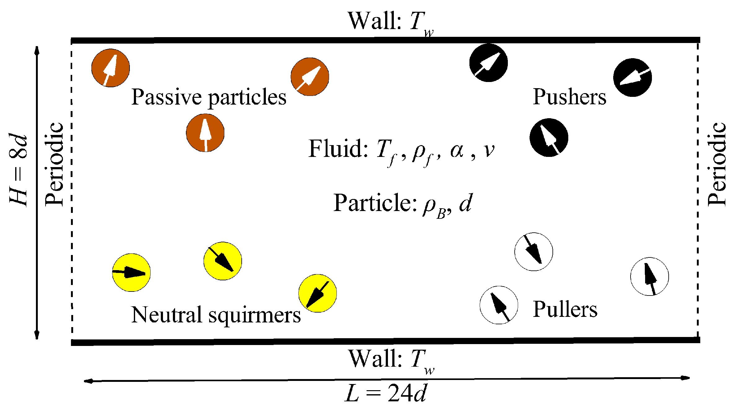
Figure 2: Diagram of the calculation model. Top and bottom of the computational domain are wall boundaries while the left and right sides display periodic boundary conditions. In order to clearly illustrate the computational model, the diagram presents the relevant coefficients for both particles and fluid. Specifically, ρ_B (particle density), d (particle diameter), T_f (temperature of the fluid), T_w (temperature of the wall), ρ_f (fluid density), ν (fluid viscosity), and α (fluid thermal diffusivity). Unless otherwise specified, the number of particles in the flow field for the simulation is forty-eight.

The diffusion coefficient of the Brownian motion reflects the self-diffusivity of the particles in the fluid and is denoted by D. The diffusion coefficients of Brownian motion are listed in the table below.

K usually denotes the analytical solution for the resistance of circular particles moving in a channel at a low Reynolds number [41]. K is defined as: K=1lnH*−0.9157+1.7244/H*2−1.7302/H*4+2.4056/ H*6 −4.5913/H*8(15) H* denotes the ratio of the channel height to the particle diameter, H* = H/d.

In the present study, in order to systematically study and analyze the group behavior of particles, three important dimensionless parameters namely λ, Pr and Le are introduced. These are defined as follows: λ=Tw−TfTw+Tf(16a) Pr=να(16b) Le=αD(16c) λ is used to indicate the relative temperature of the fluid and the channel walls. When λ = 0, a uniform temperature exists in the channel, λ > 0 indicates heating of the walls, and λ < 0 is the case of cooling of the walls. The Prandtl number (Pr) was used to measure the ratio between the momentum diffusion and thermal diffusion in the fluid, and the Lewis number (Le) was used to measure the ratio between the fluid thermal diffusion and particle diffusion.

Y* was used to quantitatively analyze the group behavior of the particles. Y*t=∑i=1n2yit−HnH(17) where yi denotes the vertical position of the ith particle in the channel and n denotes the total number of Brownian particles in the channel. Based on its definition, Y* can evidently quantitatively reflect the aggregation behavior of particles in a channel with width H. A higher value of Y* indicates that the particles are located farther away from the centerline of the channel in the vertical direction and also tend to aggregate towards the wall surface. A smaller value of Y* indicates that the particles were more aggregated in the vertical centerline of the channel.

Furthermore, to systematically analyze the effect of pushers and pushers’ own properties on group behavior, the swimming Reynolds number (Res) was used as an important dimensionless parameter. Where Res is defined as follows. Res=Usdν(18) Us denotes the self-propelling strength of the puller and pusher under steady conditions, while ν denotes the kinematic viscosity. The timescale is given by ts = d/Us.

The Reynolds number based on the velocity scale UB and the diameter of Brownian particles was introduced for the work:

The velocity scale is as follows: UB=kBTfM(20) M represents the mass of the particle. The time scale is given by tB = d/UB.

Dimensionless parameters based on the definition of the puller and pusher velocity: vs*=U2+V2UB(21) U and V denote translational velocities of the puller and pusher in the x and y directions, respectively. The time scale is t* = t/ts.

Finally, the Particles in Brownian motion in a flow field are essentially molecules with irregular thermal motion. The particles and surrounding fluid eventually reached thermal equilibrium after a long period of collision motion. Based on the theory of equalization energy, the relationship between the velocity of a Brownian particle and the temperature of the fluid is as follows: U2=V2=kBTfM(22a) Ω2=kBTfJ(22b) Ω denotes the rotational speed, and M and J denote the mass and moment of inertia of the particles, respectively.

3 Validation

3.1 Passive Particles

The accuracy of the FLBM was demonstrated in current research, and it has been applied to the simulation of the Brownian motion of particles [37,38]. To improve the reliability of the current study, sixiteen passive particles were validated to perform Brownian motion in a square computational domain (20d × 20d) at a uniform temperature. The validation results are shown in Fig. 3. As shown in Fig. 3a, it the passive particles, which are uniformly arranged in 4 × 4, display irregular arrangement after a period of diffusive motion. In Fig. 3b, the mean-square value of the velocity of the passive particles in each direction was quantitatively calculated and normalized by kBTf/M and kBTf/J. The results in the figure are sufficient to illustrate the accuracy of the validation, and the passive particles reach a thermal equilibrium state in the translational and rotational directions.

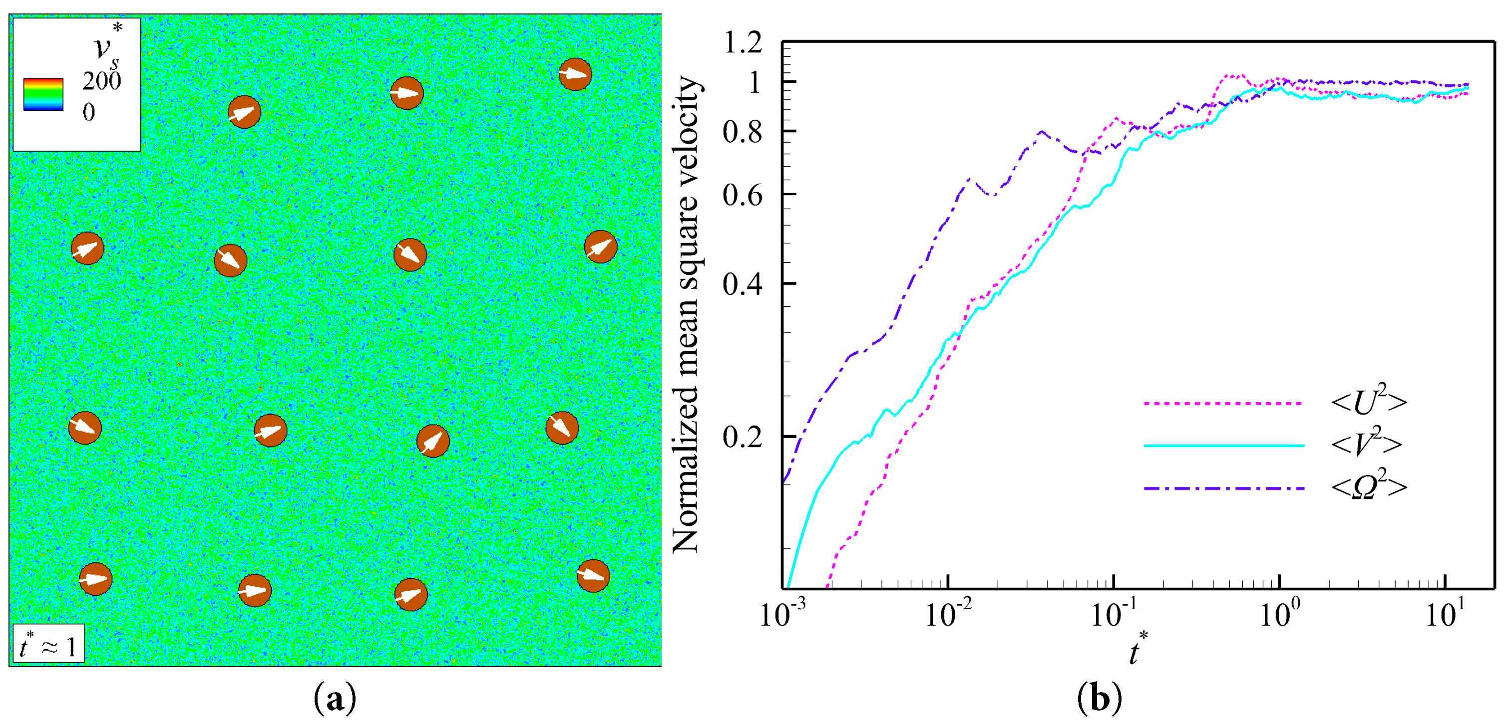
Figure 3: When Re_B = 0.067, (a) instantaneous state of 16 Brownian particles in the flow field. (b) Normalized mean squares of the translational/rotational velocity of Brownian particles. Specifically, the <U2> and <V2> are normalized by k_BT_f/M, but <Ω2> is normalized by k_BT_f/J. Instantaneous v_s* flow fields of particles plotted later share a legend with Fig. 3a.

3.2 Effect of the Wall Temperature on Passive Particle

The aggregation behavior of passive particles in variable-temperature flow fields was examined. To validate the accuracy of the heat transfer model construction, the population behavior of passive particles in heated and cooled walls was validated in the study [38]. The passive Brownian particles in the channel followed a motion pattern of diffusion from the high-temperature region to the low-temperature region. The computational model shown in Fig. 2 was adopted for validation. The results are shown in Fig. 4 as instantaneous flow-field diagrams of forty-eight passive particles for the cooled and heated walls. For the flow field diagram of multiple particles, it is mainly necessary to observe their aggregation positions. Based on the previous definition of λ, Fig. 4a shows the aggregation display of passive particles in the channel for the case of heated wall surface, and Fig. 4b shows the group behavior of passive particles in the channel for the case of cooled wall surface. Quantitative calculations were performed as shown in Fig. 5 to quantitatively demonstrate the difference between the aggregation behavior of passive particles in the cooling and heating cases, and the results were subjected to least quadratic fitting to obtain a quadratic relationship between Y* and t/tB. This further demonstrates the trendiness of the particle trajectory changes and deepens the reliability of the quantitative analysis of the results. In the subsequent analysis, we also performed a quadratic fitting analysis of Y* and t/tB, by which the regularity of the results is more intuitive. The variation of Y* over time can be clearly seen. It should be noted that in the case of the heated wall, Y* tends to increase with time (t/tB > 18) because the heat transfer in the channel causes the low-temperature region in the channel to narrow, and some of the Brownian particles enter the high-temperature region and restart their random motion. At this point, the particles need a longer period of re-motion to re-stabilize in the channel.

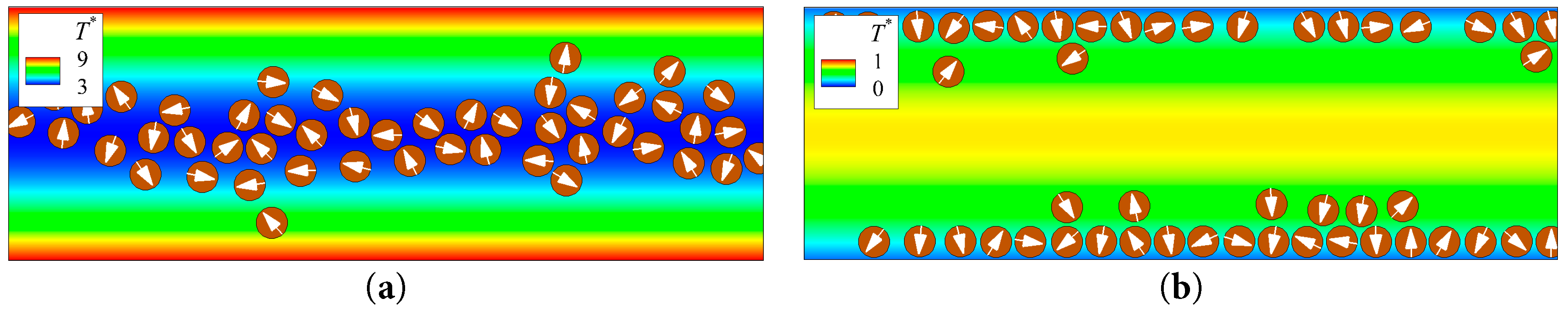
Figure 4: Different motion states of passive particles when a temperature difference exists between the wall and fluid at t* ≈ 10. (a) λ = 0.8 (Heated wall), (b) λ = −0.8 (Cooled wall). Temperature is normalized by T* = T/T_f.

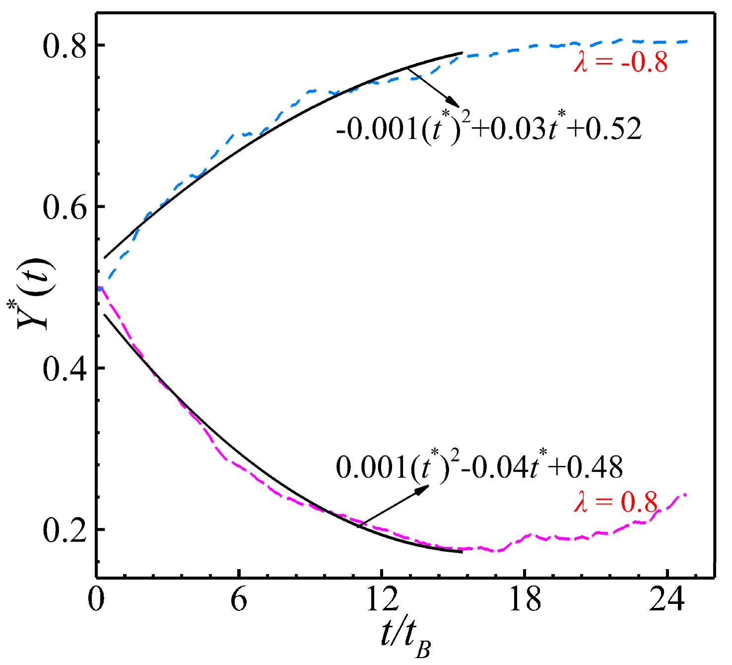
Figure 5: Time series of the averaged vertical positions for Brownian particles under different wall temperatures.

3.3 Squirmer Model

The active self-propelled Brownian particles used in the study were based on the classical Squirmer model. To verify the accuracy of the model construction, the swimming of the squirmer model with different driving modes in an unrestricted square area (60d × 60d, d = 40) was simulated. The driving mode of the puller corresponded to low pressure in the front and back and high pressure on both sides whereas the driving mode of the pusher corresponded to high pressure in the front and back and low pressure on both sides as clearly shown in Fig. 6a,c, which illustrates their differences. In addition to the pressure distributions and streamlines in the flow field, the steady velocities of the puller, pusher and neutral were calculated as shown in Fig. 7. The steady velocities were normalized using B1/2, which was in agreement with the results presented in the method and the magnitude of the steady velocities of the squirmer. The result verified the accuracy of the pulling- and pushing-type microswimmers model construction.

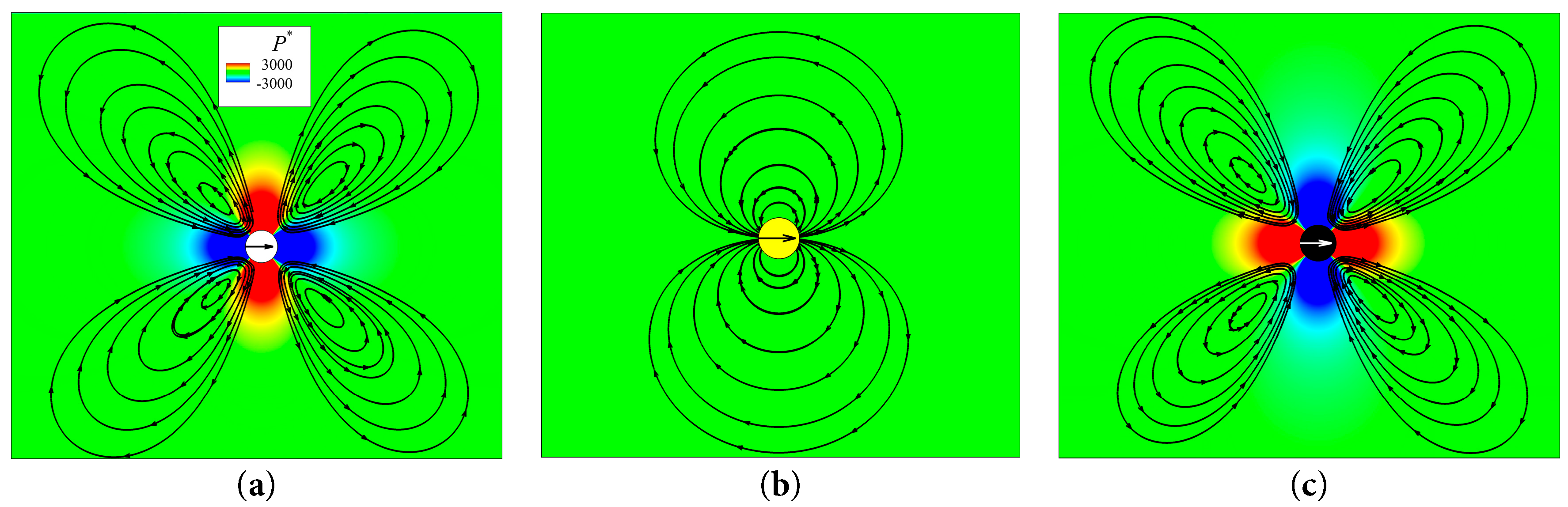
Figure 6: Flow field and streamlines of squirmers with different driving modes freely swimming in a wide region (60d × 60d). The swimming Reynolds number is 0.0005. The pressure is normalized using P* = ρ_f/(3U_s2). In all subsequent flow field diagrams, white circles with black arrows indicate puller particles and black circles with white arrows indicate pusher particles. (a) β = 3, (b) β = 0, (c) β = −3.

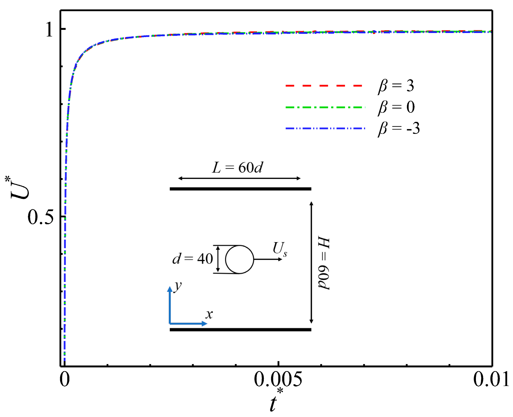
Figure 7: Motion model of a squirmer in the wide channel and the analysis graph depicting the gradually stabilized swimming velocity as time changes. The velocity is normalized using U* = U/U_s, where U_s denotes the steady-state self-propulsion speed of the squirmer.

4 Results

In this section, the aggregation behavior of forty-eight pushers or pullers in a variable-temperature flow field is discussed in detail. The discussion is divided into two cases: wall heating and cooling. The aggregation tendency of the pullers and pushers in a variable-temperature flow field is discussed in Section 4.1. The effect of the intensity of the temperature difference (λ) on the degree of the puller and pusher aggregation are discussed in Section 4.2. The effect of the swimming Reynolds number of the puller and pusher are discussed in Section 4.3. The thermal diffusivities (Prandtl and Lewis numbers) are discussed in Section 4.4. Finally, the group aggregation behavior of the pullers and pushers was summarized and analyzed.

4.1 Difference between Puller and Pusher

To visually compare the aggregated motions of the puller and pusher in a temperature-differentiated fluid, the study simulated the motions of the puller and pusher in a flow field with a heated wall, cooled wall, and uniform temperature. The heated wall cases λ = 0.8. The uniform temperature case λ = 0.0, and the cooled wall case λ = −0.8.

As shown in Fig. 8, the value of Y* for each data point is calculated separately to quantitatively analyze the motion state of the puller and pusher in the three cases. Fig. 8a shows the time series of the averaged vertical positions of the pullers and pushers for different values of β in the case of heating the wall. It is evident that both puller and pusher efficiently aggregated towards the center of the channel without any difference in the aggregation trends. This is consistent with the movement of passive Brownian particles from high-to low-temperature regions as shown in Fig. 5. Fig. 8b shows the time series of the averaged vertical positions of the pullers and pushers in a uniform temperature flow field, where there are some slight differences: the pullers tend to converge towards the center of the channel, and the pushers tend to move towards the wall. The closer the value of β is to zero, the more similar the puller and pusher motion trend is to the neutral, exhibiting unbiased diffusive motion. As shown in Fig. 8c, on the cooled wall surface, the motion trends of the pullers and pushers exhibit a more noticeable distinction. It can be observed that for the pusher, irrespective of the value of β, its motion trend is consistently towards wall aggregation. In contrast, for the puller, the tendency is to aggregate towards the wall only when the value of β is close to zero. This can be visualized in Fig. 9 by the flow field diagrams. Additionally, we placed the pullers and pushers in the flow field at the cooled wall surface to observe their aggregation motion. Thus, the difference between the motion trends of the pullers and pushers is clearly shown in Fig. 10 with the pushers displaying a strong pro-wall surface and the pullers displaying a far-wall surface. The verification section has clearly demonstrated the differences among various Squirmers. Based on the driving mechanisms, the puller generates low pressure in the front and back and high pressure on the sides whereas the pusher generates high pressure in the front and back and low pressure on the sides. When a pusher gets close to a wall, it reorients itself parallel to the wall and the lower pressure nodes generated on its sides attract it to the wall. It can be seen in Fig. 9b. For a puller the exact opposite mechanism drives the swimmer away from the wall and towards the middle of the channel.

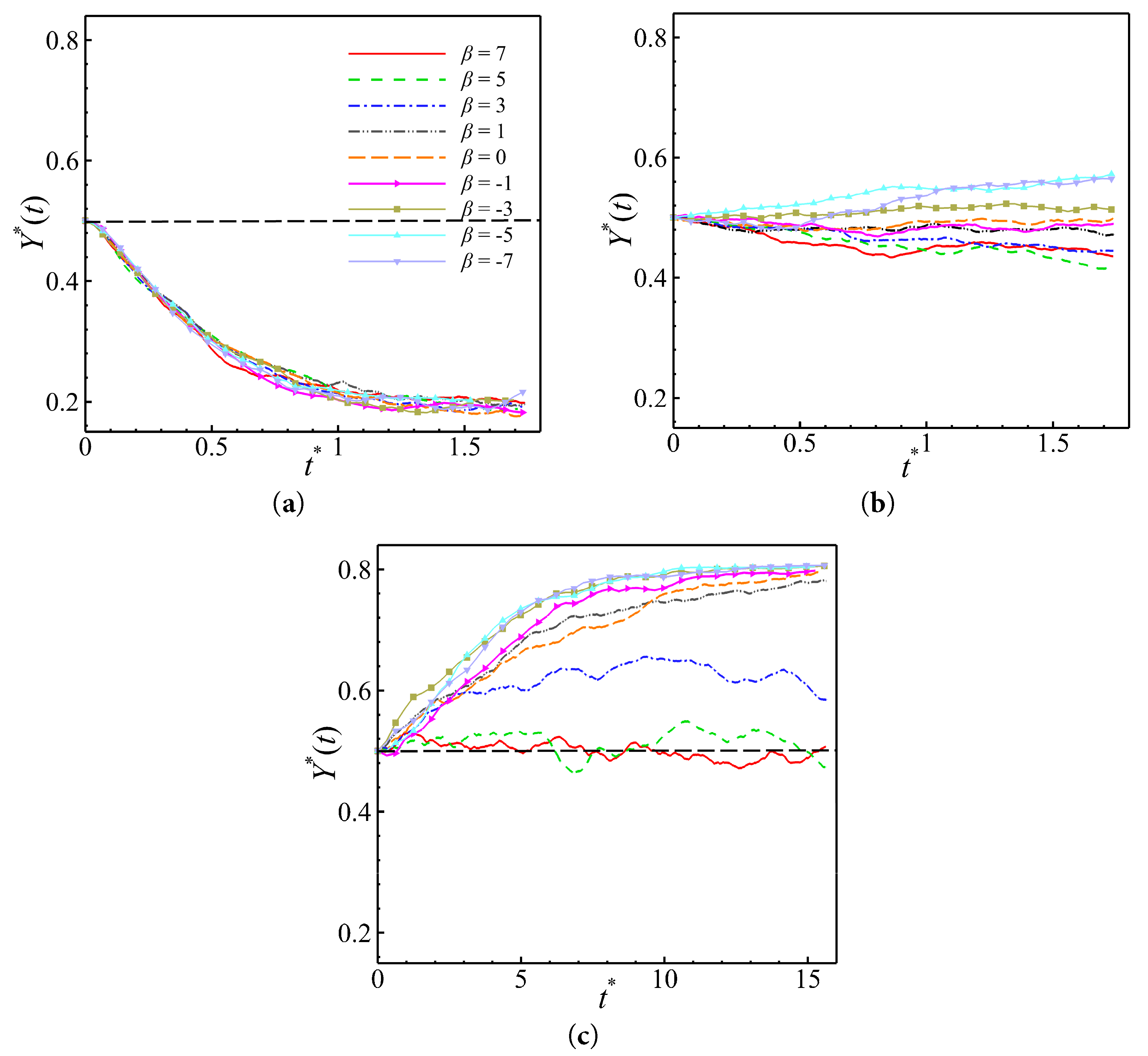
Figure 8: Time series of the averaged vertical positions for pullers and pushers with different values of β under different wall temperatures: (a) λ = 0.8, (b) λ = 0, (c) λ = −0.8.

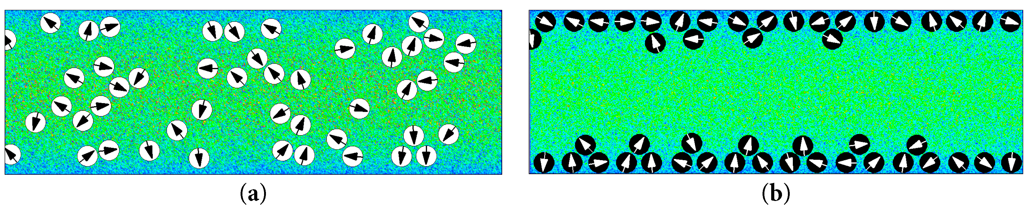
Figure 9: Instantaneous flow fluctuations and distributions of the pullers and pushers in the channel (λ = −0.8) for different values of β at t* ≈ 14: (a) β = 7, (b) β = −7.

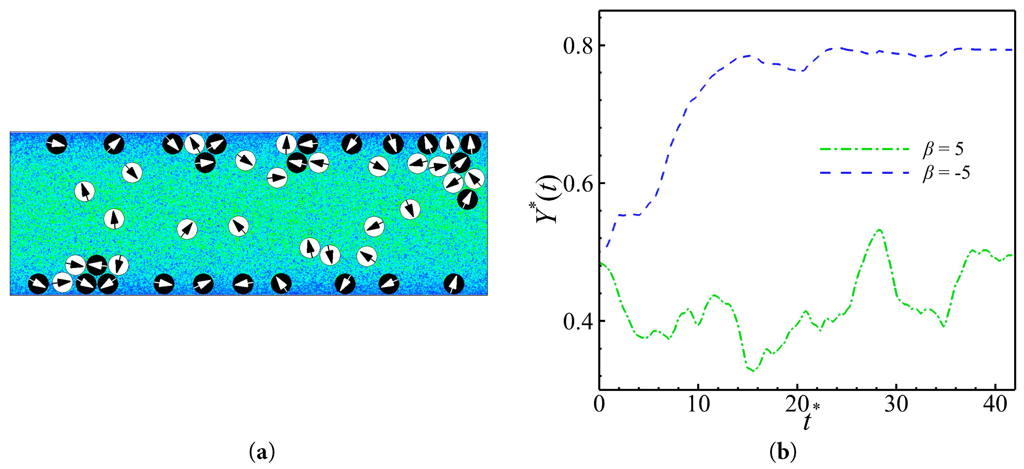
Figure 10: When puller (β = 5) and pusher (β = −5) are located in a channel with λ = −0.8: (a) Instantaneous flow field. (b) Time series of the averaged vertical position.

However, pullers with different values of β exhibit varying degrees of aggregation on the cooled wall surface. This is because increases in the value of β lead to differences in the tangential peak velocity of the puller’s surface motion, leading to different behaviors in the flow field. This is verified in Fig. 11, which shows the state of pressure distribution in the flow field for puller and pusher at a very low value of Res (Res = 0.0005). At a constant pressure difference, it is evident that increases in the value of β increase the pressure distribution range of the puller as shown in Fig. 11a. The pusher shown in Fig. 11b is also in line with this argument where increases in the value of β increase the pressure distribution range. This implies that given a constant differential pressure, the widening of the pressure region makes the pusher more likely to be sucked by the wall whereas the puller is more likely to bounce off the wall. The computational results in Fig. 8 confirm that irrespective of close the value of β is to zero, the puller is far inferior to pusher in terms of aggregation towards the wall in the presence of cooler walls. Given the above conclusions, the aggregation motion of the puller in the case of a cooled wall surface is not discussed in the study. Only the factors that affect the aggregation of the puller at the center of the channel in the case of a heated wall were discussed.

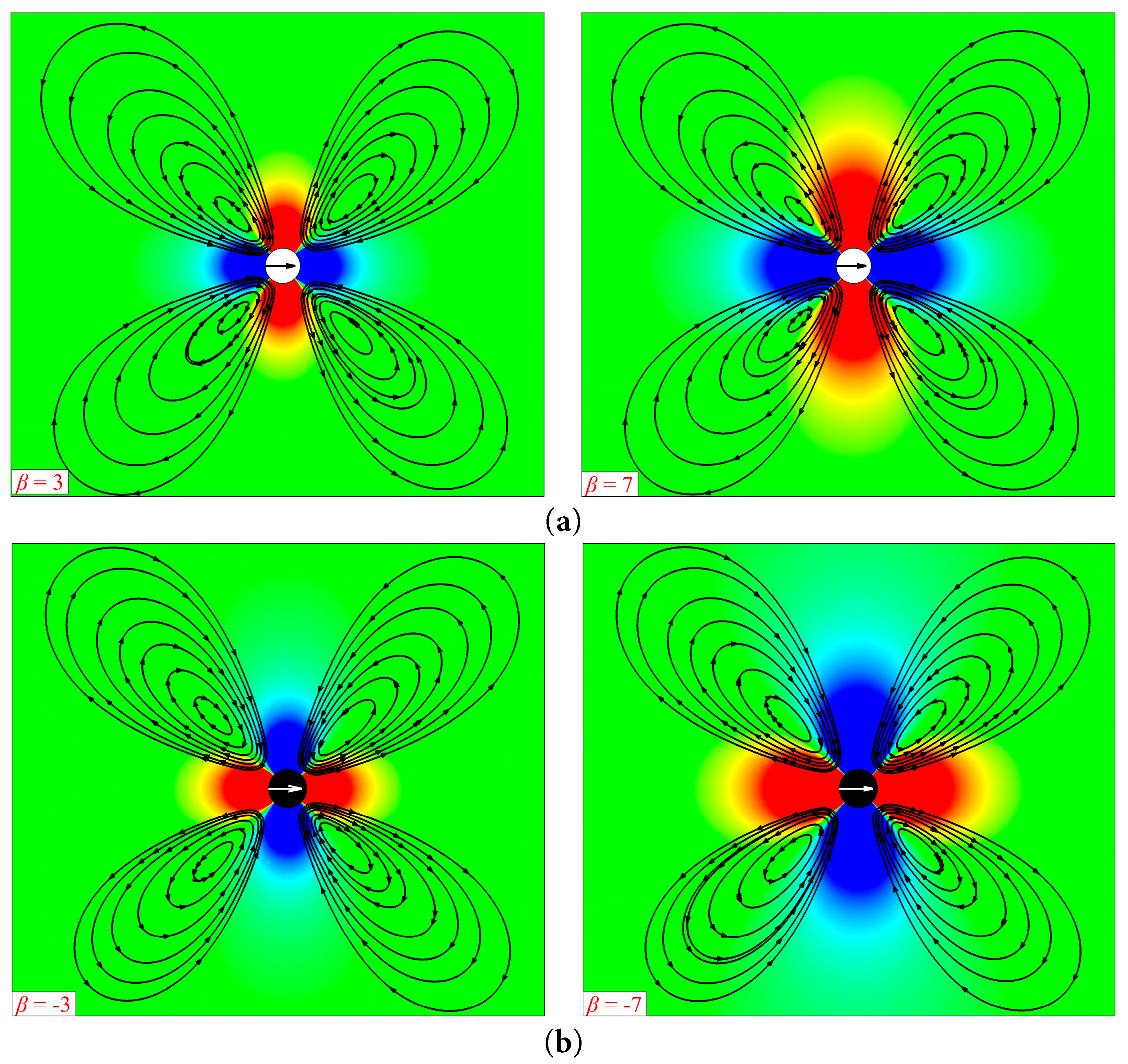
Figure 11: Same conditions as in Fig. 6. Flow field and streamlines of the puller and pusher freely swimming in a wide region (60d × 60d). (a) β > 0 (puller), (b) β < 0 (pusher).

4.2 Effects of Wall Temperature

As shown in Section 4.1, the effect of the temperature difference on the aggregation behavior of the pullers and pushers is very significant, and the effect of different temperature intensities on the pullers and pushers is analyzed and investigated in this section, in which the temperature difference in the flow field is changed by heating or cooling the wall.

This section discusses two main cases: heating and cooling of the wall. In this section, the effects of different temperature difference intensities on the aggregation properties of the puller and pusher are discussed. We analyze the effect of temperature difference intensity (with respect to the numerical magnitude of λ, increases in the λ increase the temperature difference intensity) on the puller aggregation behavior by the value of Y*. Aggregation performance and efficiency are defined based on the magnitude and time of the minimum value that Y* can reach. The time series of the averaged vertical position of the pullers with different temperature intensities was quantitatively calculated for a heated wall, as shown in Fig. 12. The computational fit clearly shows the changing state of Y* with t*. As shown in Fig. 12, increases in the value of λ improve the aggregation performance of the puller. In addition, aggregation efficiency did not increase with increases in the temperature difference. The aggregation efficiency of the puller is not affected by λ, and this is related to its own aggregation properties as demonstrated in Section 4.1. In the instantaneous flow field diagram shown in Fig. 13, it can be visualized that the aggregation performance of the puller is stronger in the flow field with a stronger temperature difference at the same moment.

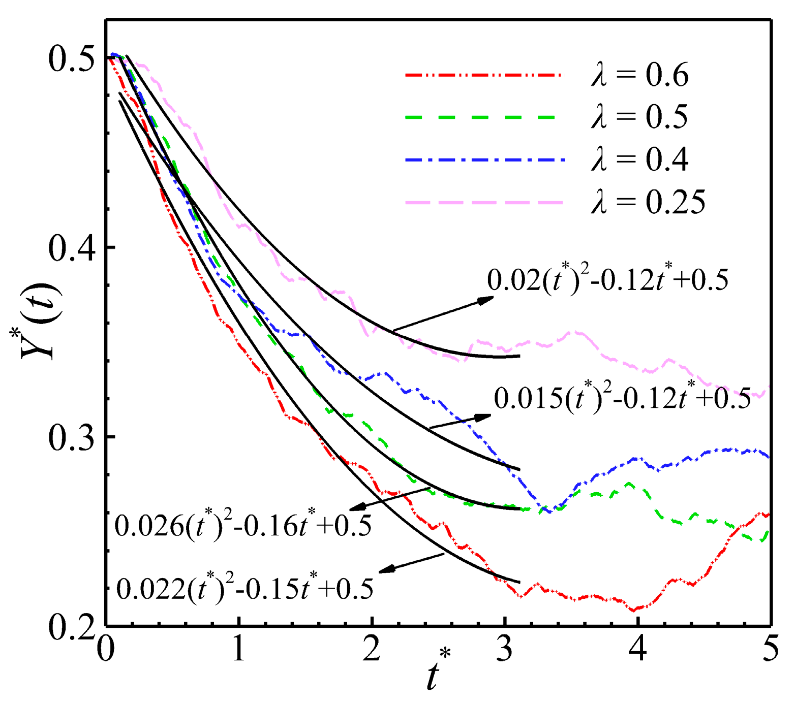
Figure 12: In the case of a heated wall, time series of the average vertical positions of the pullers (β = 5) at different values of λ.

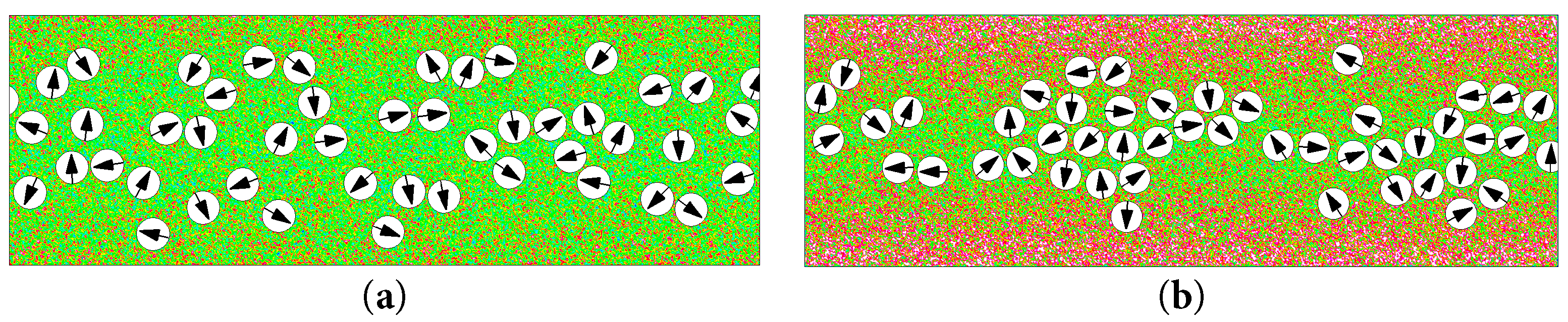
Figure 13: Instantaneous flow fluctuations and distributions of the pullers (β = 5) in the channel for different values of λ at t* ≈ 5. (a) λ = 0.25, (b) λ = 0.6.

Time series of the average vertical positions of the pushers were calculated as shown in Fig. 14 for the heated wall case for different values of λ. The quadratic relationship between Y* and t* was fitted and the state of change of Y* with t* can be clearly seen through the results. It can be observed that when λ is relatively small, it is unable to drive pushers to aggregate towards the center of the channel. However, the pushers do not follow their own aggregation characteristics to aggregate towards the wall surface. This indicates that under this temperature-difference intensity, the pushers are in a state of random diffusion, with temperature-difference-driven and self-propelled characteristics in a balanced state. Increases in the value of λ increase the efficiency and performance of pusher aggregation towards the center of the channel. This is because increases in the value of λ makes the thermal fluctuation of the flow field is stronger and the pusher is subjected to stronger Brownian motion. The instantaneous flow field diagrams are shown in Fig. 15 and clearly demonstrate that increases in the value of λ improves the aggregation of pushers at the center of the channel. This can be easily observed by comparing Fig. 15a,b. It should be noted that the time series of the average vertical positions of the pullers and pushers in Fig. 12 and Fig. 14 exhibit a fluctuating tendency to increase after a period of diffusive motion (t* > 3) and after the value of Y* has reached a minimum. This is because the heat transfer of temperature in the channel leads to the narrowing of the low-temperature region in the channel, and some pullers and pushers enter the high-temperature region and start moving randomly again. At this point, the particles need a longer period of re-motion to re-stabilize in the channel.

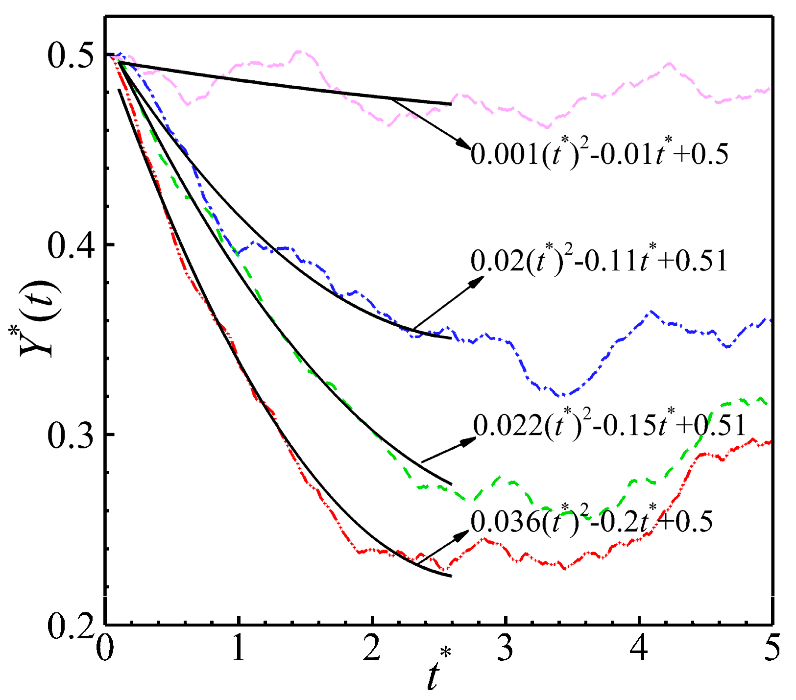
Figure 14: Same conditions as in Fig. 12. In the case of a heated wall, time series of the average vertical positions of the pushers (β = −5) at different values of λ.

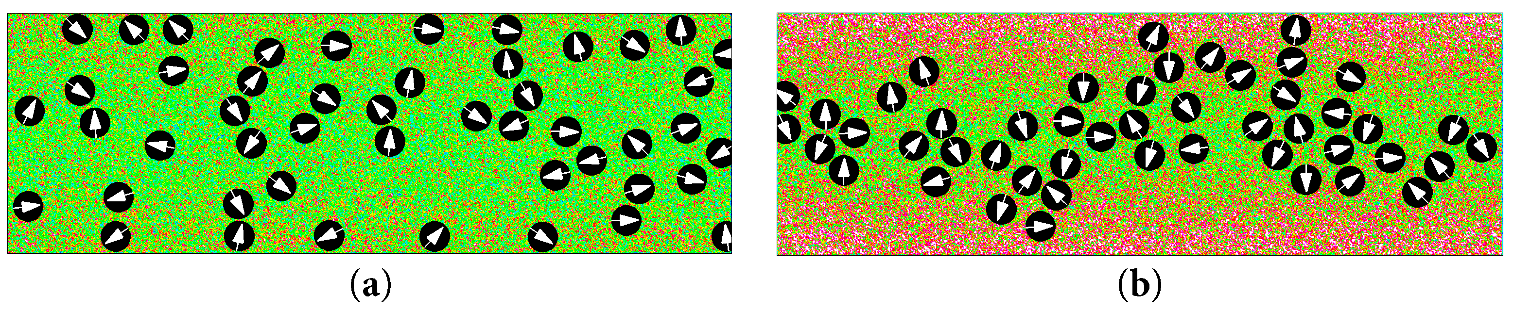
Figure 15: Instantaneous flow fluctuations and distributions of the pushers (β = −5) in the channel for different values of λ at t* ≈ 5. (a) λ = 0.25, (b) λ = 0.6.

In Fig. 16, the time series of the average vertical positions of the pushers was calculated when the wall was cooled. The pushers rapidly aggregate towards the wall when the wall is cooled. Increases in the temperature difference increase the aggregation efficiency of the pusher. However, the difference in the aggregation efficiency was not significant. This is because the population behavior of the pushers when cooling the wall surface shows aggregation towards the wall surface. Eventually, all the pushers aggregate near the wall surface. Therefore, it is impossible to analyze the effect of the temperature difference on the aggregation performance. Overall, increases in the intensity of the temperature difference, enhances the aggregation of the pullers and pushers during heating as well as cooling the wall.

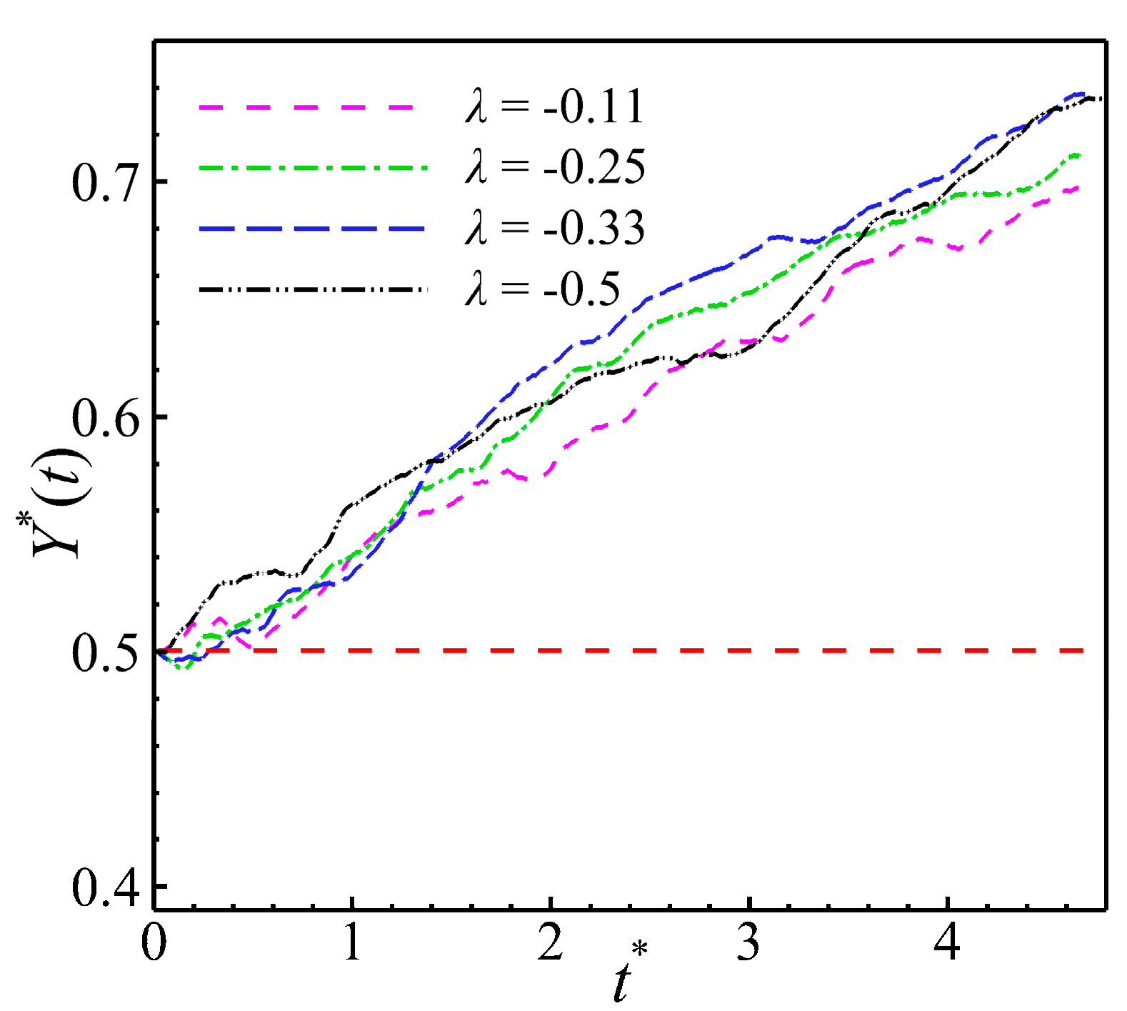
Figure 16: In the case of a cooled wall, time series of the average vertical positions of the pushers at different values of λ.

4.3 Effects of Swimming Reynolds Number

Given the use of the pullers and pushers as active Brownian particles, it is essential to consider whether the swimming Reynolds number of the puller and the puller itself affects its aggregation properties. In this section, we discuss the manner in which the aggregation properties of the puller and pusher differ for different values of Res via adjusting its self-propelling strength. In this section, we analyze the effect of the swimming Reynolds number through the value of Y*. Aggregation performance and efficiency are defined based on the magnitude and time of the minimum value that Y* can reach.

In Fig. 17, the time series of the averaged vertical positions of the pullers is calculated for the case of a heated wall. As shown in Fig. 17, for the pullers, increases in the value of Res increase the aggregation efficiency whereas the corresponding aggregation performance decreases. This is because increases in the self-propelling strength of the pullers increase the swimming Reynolds number. In the flow field on the heated wall, the temperature difference drives the pullers to aggregate towards the center of the channel at a higher velocity, resulting in a higher aggregation efficiency. However, the decrease in aggregation performance is potentially because the rapid aggregation of the pullers towards the center of the channel results in a higher velocity for each puller particle within the narrow and finite central region. The collisions between particles became more intense, and thus it easier for the pullers to be ejected from the central region during these collisions. As shown in Fig. 18, it is observed from the instantaneous flow field diagram that pullers with higher value of Res exhibit inferior aggregation performance compared to those with lower value of Res.

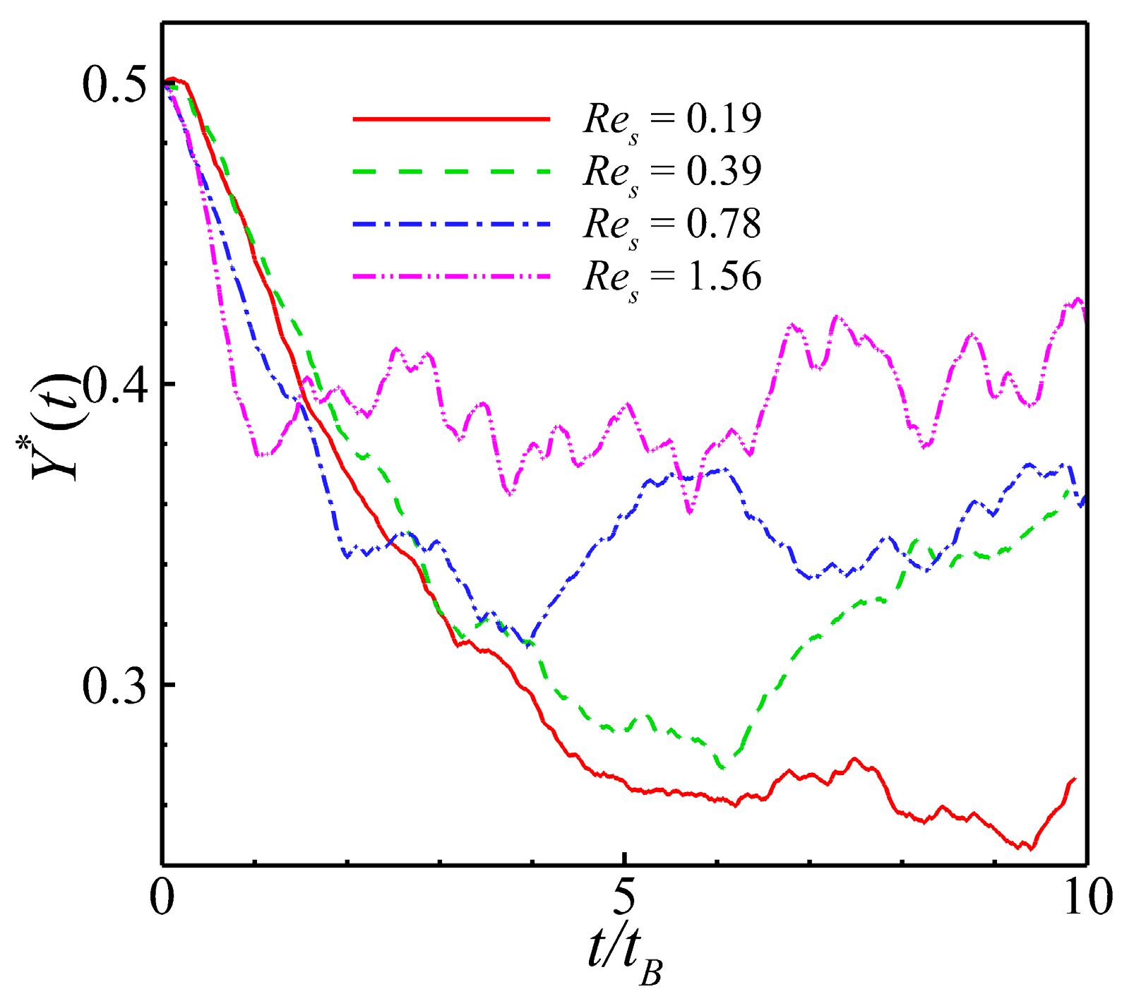
Figure 17: Time series of the averaged vertical positions of the pullers are calculated for different values of Re_s at λ = 0.5.

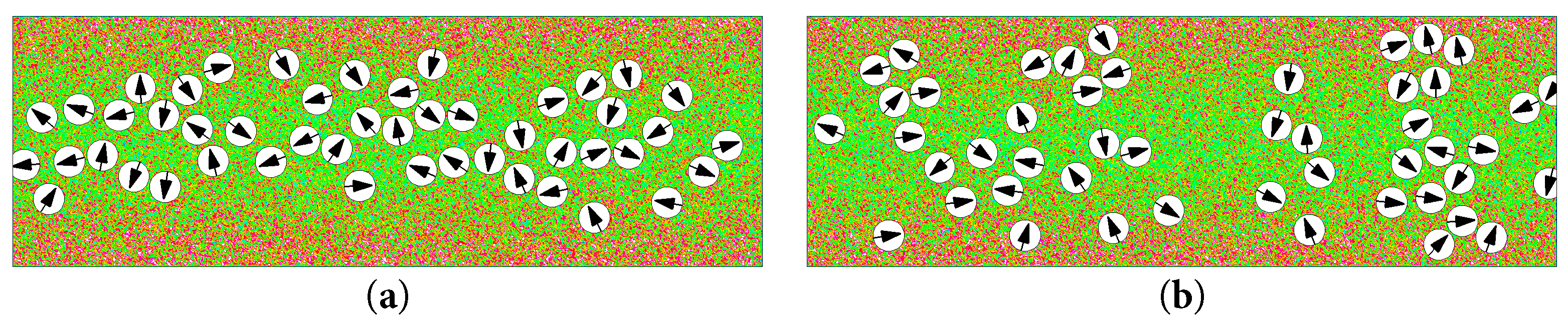
Figure 18: In the case of a heated wall (λ = 0.5), instantaneous flow fluctuations and distributions of the pullers (β = 5) in the channel for different values of Re_s at t/t_B ≈ 10. (a) Re_s = 0.19, (b) Re_s = 1.56.

Interestingly, the aggregation performance of the pusher in Fig. 19 is different for different sizes of Res. We performed a least-squares fitting of the value of Y* and the state of change of Y* with t* can be clearly seen through the results. When the value of Res was relatively low, the pushers tended to aggregate towards the center of the channel. However, when the value of Res increases, the pushers no longer demonstrated a tendency to aggregate towards the channel center. After the value of Res reaches a certain threshold, the pushers break free from the effect of the temperature difference and start aggregating towards the wall surface. This is because in our simulation, we used the random thermal motion of molecules driven by the temperature difference to induce the aggregation behavior of the pullers and pushers. However, when the self-propelling strength of the pushers becomes dominant at a sufficiently high value of Res, their propulsion dominates the motion. Therefore, the aggregation characteristics of the pushers with high value of Res in the flow field are determined by their properties. This means that even in the case of a heated wall, the pushers will still aggregate towards the wall surface when the value of Res is high. Furthermore, in the flow field diagrams shown in Fig. 20, distinct aggregation patterns can be observed for pushers with different values of Res.

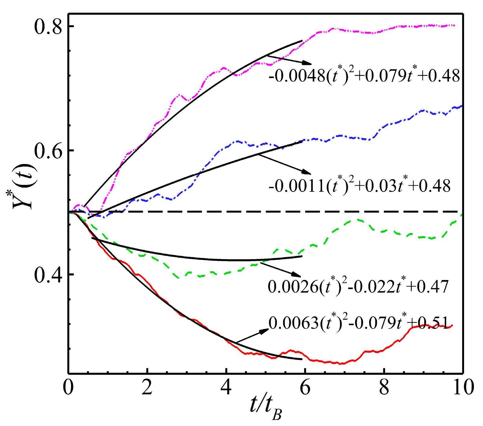
Figure 19: Same conditions as in Fig. 17. In the case of a heated wall (λ = 0.5), time series of the averaged vertical positions of the pushers at different values of Re_s.

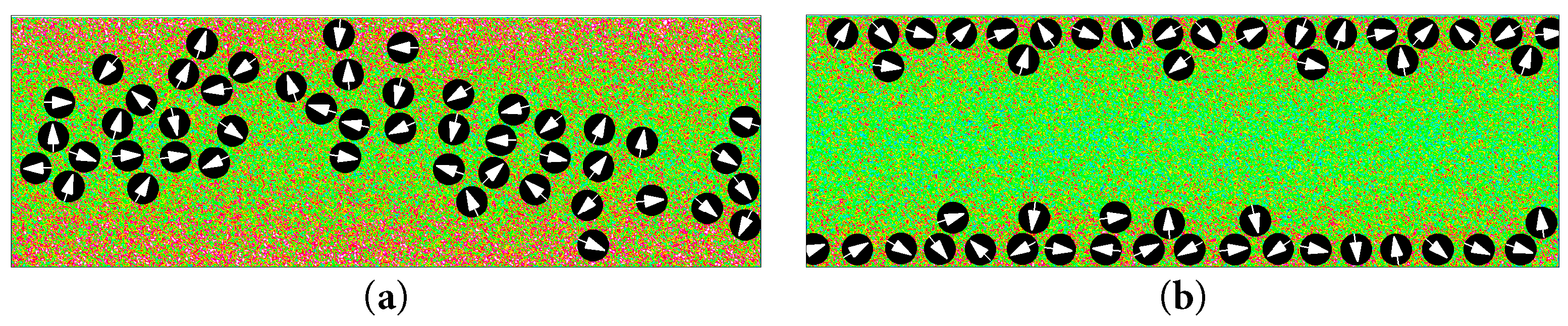
Figure 20: In the case of a heated wall (λ = 0.5), instantaneous flow fluctuations and distributions of the pushers (β = −5) in the channel for different values of Re_s at t/t_B ≈ 10. (a) Re_s = 0.19, (b) Re_s = 1.56.

In Fig. 21, the time series of the averaged vertical positions of the pushers on the cooled wall surface were calculated, and a least-squares fitting of the value of Y* was performed. In the case of a cooled wall surface, increases in the value of Res increases the efficiency of the pusher aggregation towards the wall surface. This is because pushers with higher velocities diffuse towards the wall surface more rapidly. The increase in the pusher aggregation efficiency follows the same trend as that observed in the other cases.

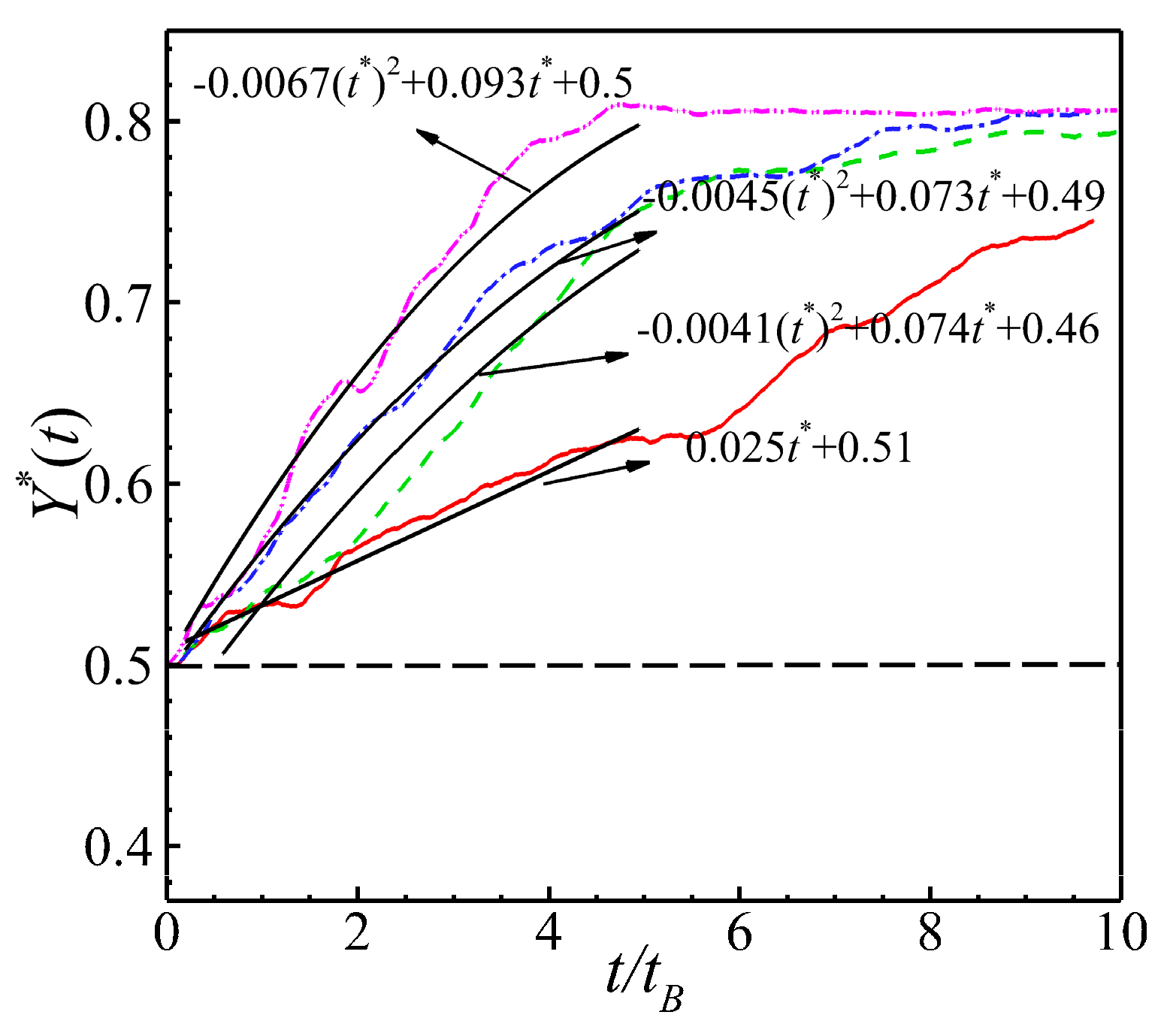
Figure 21: The same conditions of Fig. 17. Time series of the averaged vertical positions of the pushers are calculated for different values of Re_s at λ = −0.5.

4.4 Effects of Thermal Diffusion

In the study, heat transfer terms were introduced into the flow field based on the analyses conducted in the previous chapters. The collective motion of the pullers and pushers within a channel is significantly affected by the heat transfer process in the fluid. To address the issue, this section discusses the effect of thermal diffusion. In this section, variations in the fluid thermal diffusivity (α) and fluid viscosity (ν) are considered, leading to changes in the Prandtl and Lewis numbers.

The discussion in this chapter mainly focuses on the effect of fluid thermal diffusion on the aggregation of the puller and pusher. Therefore, the aggregation of the pusher in the cooled-wall case is first discussed. The effects of two important parameters, Pr and Le, were analyzed. As shown in Fig. 22, the aggregation behavior of the pusher is demonstrated via changes in Prandtl and Lewis numbers caused by changing the value of the ν, and the pusher exhibits stable aggregation towards the wall. As shown in the calculations in Fig. 22, it can be concluded that decreases in the value of Pr improve the aggregation efficiency of the pusher. This is because, decreases in the value of the ν decrease the value of Pr, and a lower value of the ν also indicates a lower diffusion resistance. Decreases in the resistance make the diffusion of the puller and pusher faster such that the aggregation efficiency increases. This can be observed more intuitively in Fig. 23, where a comparison of Fig. 23a,b at the same moment in time demonstrate that decreases in the value of Pr increase the aggregation efficiency of the pusher. The effect of Prandtl number on the pusher aggregation efficiency is corroborated. Fig. 24 shows the results of varying Prandtl and Lewis numbers by adjusting the value of the α. As shown in Fig. 24, decreases in the value of Pr increase the aggregation efficiency of the pushers. This is because the decrease in the value of Pr is caused by an increase in the value of the α, which leads to greater random forces acting on the pusher throughout the flow field. Thus, the pushers are able to aggregate more rapidly in the flow field. This further supports the idea that decreases in the value of Pr in the flow field increase the aggregation efficiency of the pushers.

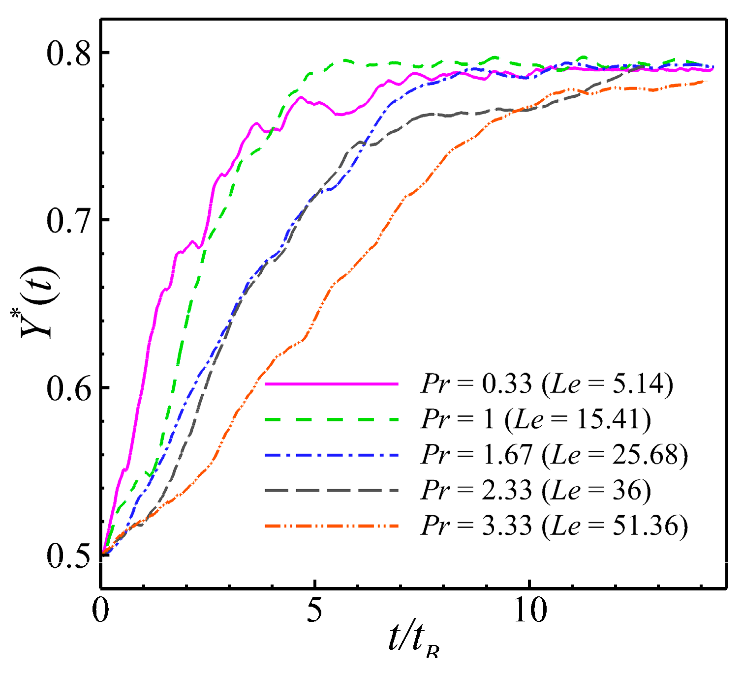
Figure 22: Time series of the averaged vertical positions of the pushers (β = −5) at different values of Pr and Le under the condition of a cooled wall (λ = −0.8). Note that Pr and Le varied based on the variation in fluid viscosity (ν).

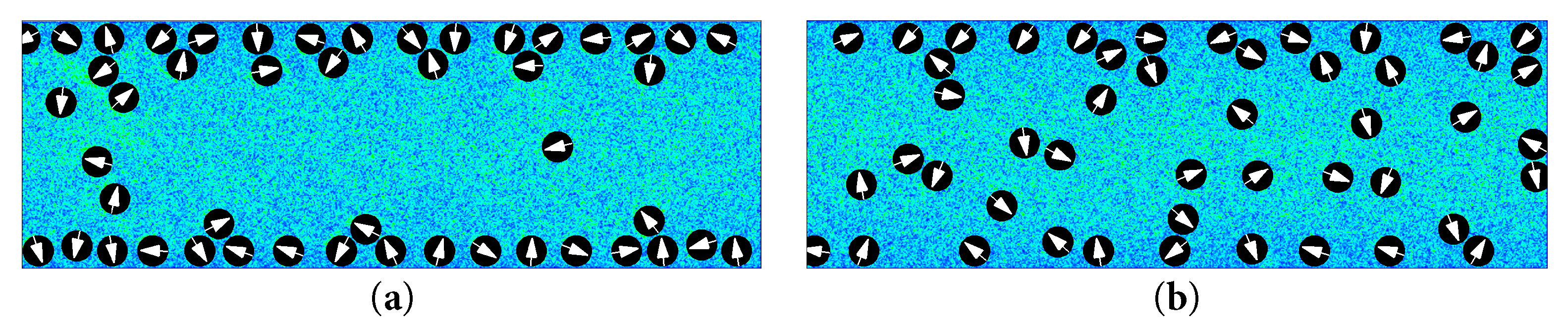
Figure 23: In the case of a cooled wall (λ = −0.8), instantaneous flow fluctuations and distributions of the pushers (β = −5) in the channel for different values of Pr and Le at t/t_B ≈ 3. (a) Pr = 0.33 (Le = 5.14), (b) Pr = 3.33 (Le = 51.36).

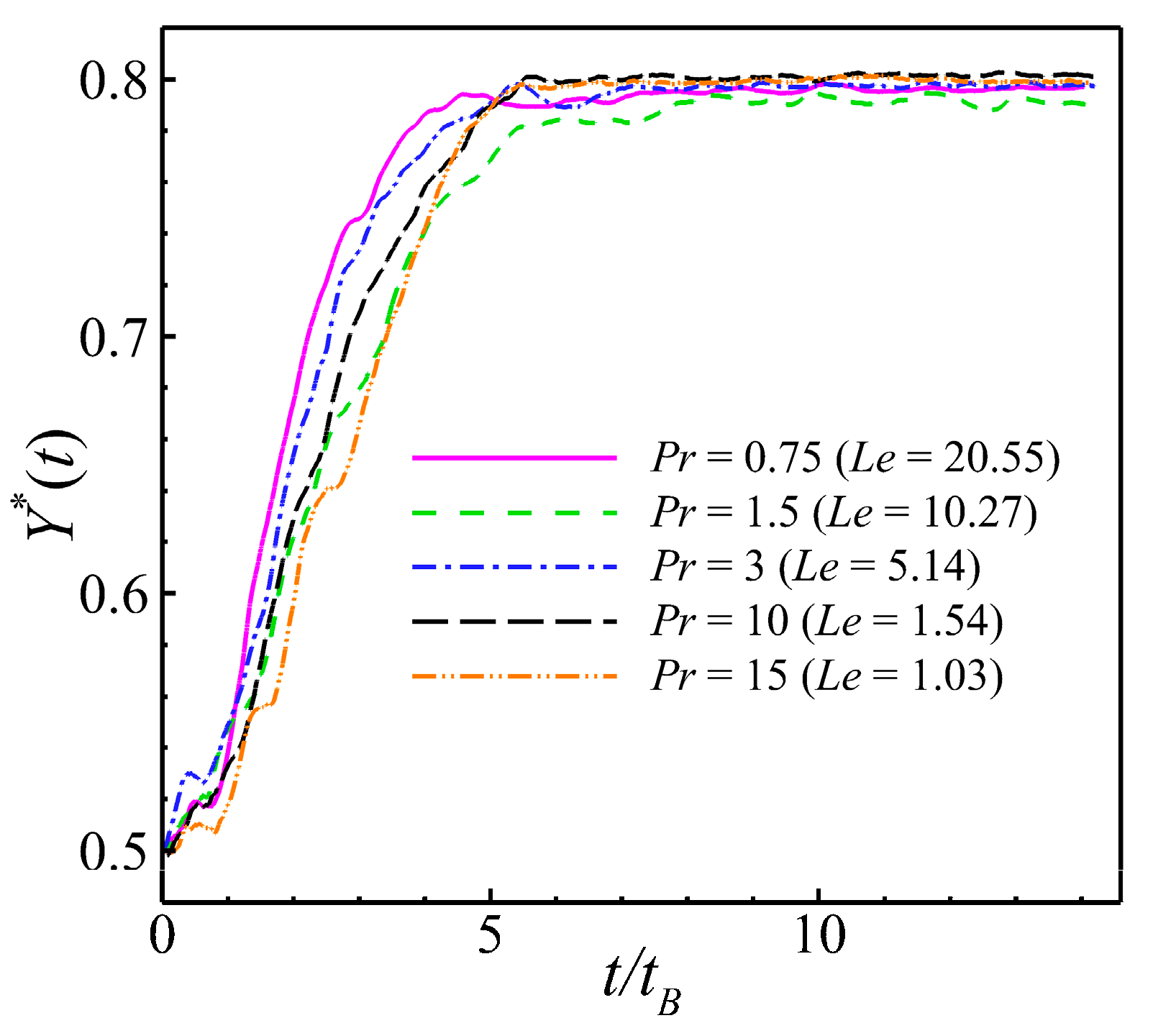
Figure 24: Time series of the averaged vertical positions of the pushers at different values of Pr and Le under the condition of a cooled wall (λ = −0.8). Note that Pr and Le varied based on the variation in thermal diffusivity (α).

It is not possible to discuss the effect of cooled walls on the aggregation properties of the pusher. Because, all pushers are sucked up by the wall eventually. To investigate the issue, the effects of changes in Prandtl and Lewis numbers on the aggregation properties of pullers and pushers in heated walls were examined. The effects of changing the thermal diffusivity of the heated wall on the aggregation state of the pullers and pushers are shown in Fig. 25. It can be observed that for the puller and pusher, decreases in the value of Pr improve aggregation efficiency and decreases in the value of Le improve aggregation performance. The principle of the Prandtl number for influencing the efficiency of the pullers and pushers was introduced earlier. Based on the definition of Le in the previous section, the effect of Le on the aggregation performance of the puller and pusher can be realized by controlling the ratio between the thermal diffusion of the fluid and the self-diffusion of particles. When the value of Le was low, the rate of thermal diffusion of the fluid was lower than the rate of diffusion of the particles. Therefore, the particles were given sufficient time to aggregate. Conversely, when Le is high, heat transfer is rapid, and the fluid in the channel is rapidly heated. In this case, the flow field already corresponds to a uniform temperature flow field prior to when the pullers have completed their aggregation. As shown in Fig. 26, the instantaneous flow field was plotted at the same moment for different values of Pr and Le. A comparison of Fig. 26a,b clearly indicate that the fluid diffusion is significantly faster with time for larger values of Le, and the particles do not have time to complete their aggregation behavior, thereby leading to a degradation of their aggregation performance.

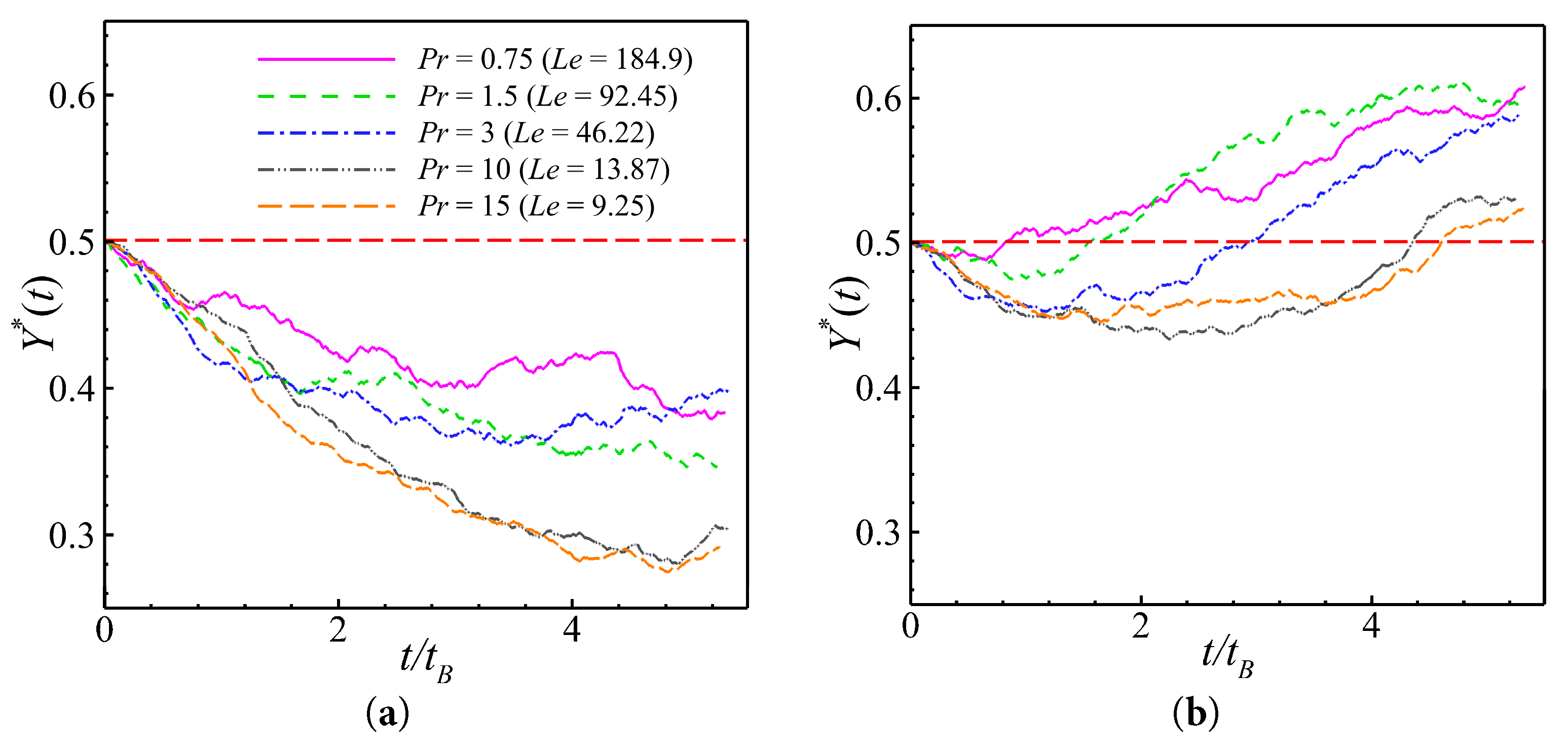
Figure 25: Time series of the averaged vertical positions of the pullers and pushers at different values of Pr and Le under the condition of a heated wall (λ = 0.8). Note that Pr and Le varied based on the variation in thermal diffusivity (α). (a) β = 5, (b) β = −5.

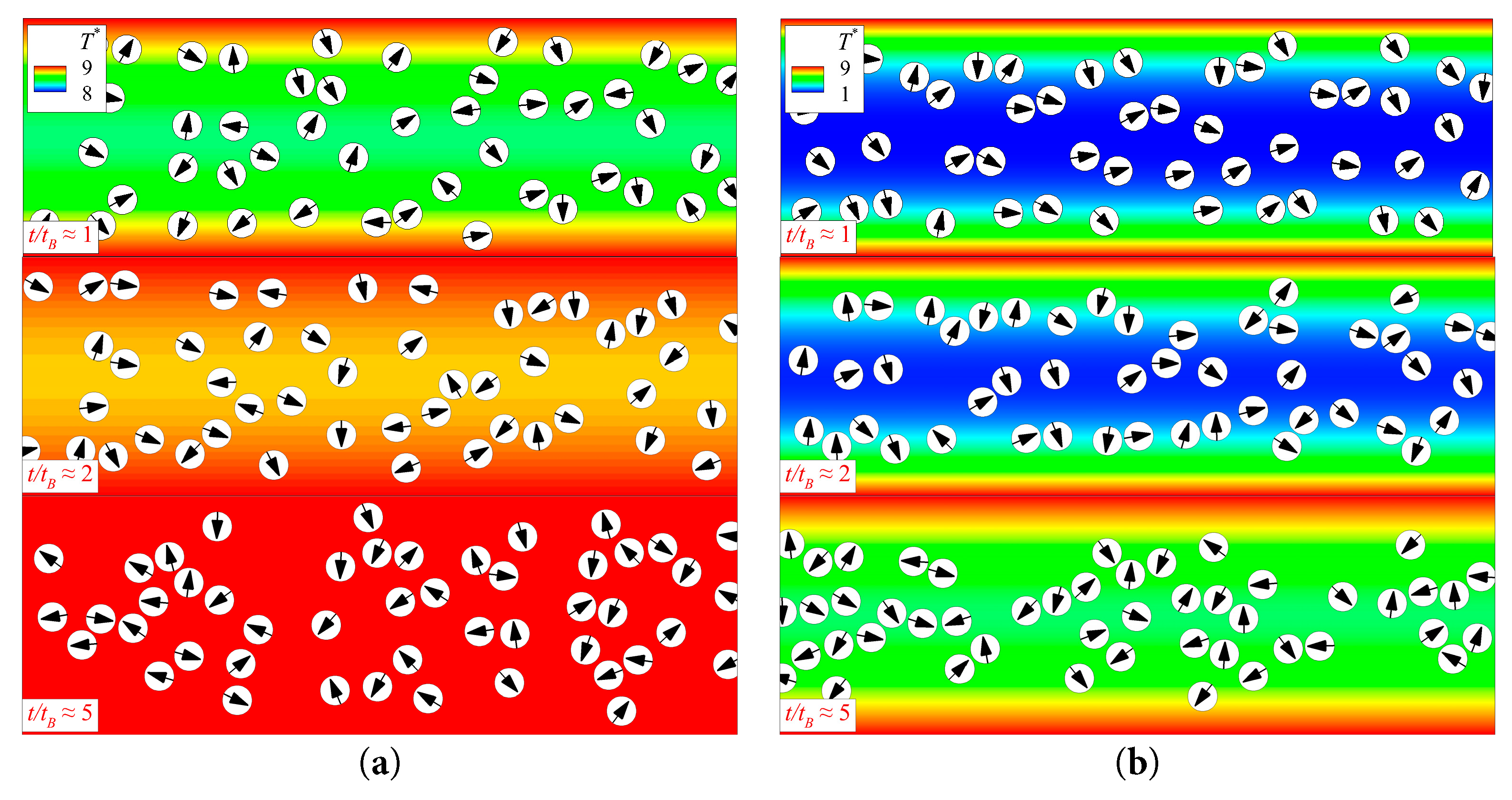
Figure 26: In the case of a heated wall (λ = 0.8) instantaneous flow fluctuations and distributions of the pullers in the channel for different values of Le and Pr at different t/t_B. (a) Pr = 0.75 (Le = 184.9), (b) Pr = 15 (Le = 9.25).

5 Conclusion

In the study, the aggregation behavior of a group of pulling- and pushing-type microswimmers in a variable-temperature flow field was investigated via a two-dimensional FLBM numerical simulation. The puller and pusher are discussed separately in the discussion of the work. The discussion on the pullers focuses on heated walls and analyzes their aggregation behavior towards the center of the channel. For the pushers, the cases of heated and cooled walls are discussed separately, and the two behavioral patterns of the pusher aggregation towards the center of the channel and wall aggregation are discussed separately. The effects of the driving mode, temperature difference, driving speed of the pullers and pushers, and fluid thermal diffusion efficiency were considered from the perspective of the focusing performance and efficiency of the pullers and pushers throughout the study. The following conclusions were obtained.

• (1)When examining the aggregation behavior of a squirmer in a temperature-differential flow field, it is essential to consider aggregation differences between the puller and pusher in the analysis. In the flow field at the heated wall, the pullers and pushers aggregated towards the center of the channel. Conversely, in the flow field at the cooled wall, a clear divergence exists in the movement tendency of the puller and pusher. The puller exhibits a far-wall character, whereas the pusher displays a pro-wall character. This was determined via the different driving principles of the puller and pusher.
• (2)In the case of the wall temperature change, increases in the temperature difference improve the aggregation performance of the puller. For the pusher, increases in the temperature difference improve the aggregation efficiency and aggregation performance. Overall, the intensity of the high temperature difference enhanced the puller and pusher aggregation.
• (3)In the discussion of the swimming state of particles, when heating the wall surface, increases in the value of the swimming Reynolds number increase in aggregation efficiency of the puller, although the aggregation performance of the puller decreases with increases in the value of the swimming Reynolds number. If the value of the swimming Reynolds number is low, the pusher will aggregate towards the center of the channel. However, if the value of the swimming Reynolds number is high, the pusher aggregates towards the wall to eliminate the effect of the temperature difference. When the wall was cooled, the aggregation efficiency of the pusher increased with an increase in the swimming Reynolds number.
• (4)The discussion on fluid diffusion and particle diffusion intensity mainly focused on Prandtl and Lewis numbers. The aggregation efficiency and performance of the pullers and pushers are primarily determined by Prandtl and Lewis numbers, assuming that the other conditions remain unchanged. Specifically, the aggregation efficiency and performance of the pullers improved when Prandtl and Lewis numbers decreased. Conversely, for pushers, a lower value of the Prandtl number leads to higher aggregation efficiency irrespective of the temperature difference. However, when considering that heating the wall causes the pushers to aggregate towards the center of the channel, it can be concluded that a lower value of the Lewis number corresponds to a better aggregation performance for the pushers.

In conclusion, this paper conducts a thorough discussion on the aggregation of particles in two-dimensional multiple squirmer models. The research in this paper provides certain reference for the particle aggregation behavior of nanofluids and water quality evolution. Due to the limitations of computing power, the research in this paper is confined to two-dimensional space. Further studies on the thermal aggregation characteristics of three-dimensional particles will be considered in the future.

References

1. Orozco J, García-Gradilla V, D’Agostino M, Gao W, Cortes A, Wang J. Artificial enzyme-powered microfish for water-quality testing. ACS Nano. 2013;7(1):818–24. doi:10.1021/nn305372n. [Google Scholar] [CrossRef]
2. Huang TY, Gu H, Nelson BJ. Increasingly intelligent micromachines. Annu Rev Control Robot Auton Syst. 2022;5(1):279–310. doi:10.1146/annurev-control-042920-013322. [Google Scholar] [CrossRef]
3. Zhou H, Dong G, Gao G, Du R, Tang X, Ma Y, et al. Hydrogel-based stimuli-responsive micromotors for biomedicine. Cyborg Bionic Syst. 2022;2022:9852853. doi:10.34133/2022/9852853. [Google Scholar] [CrossRef]
4. Ramaswamy S. The mechanics and statistics of active matter. Annu Rev Condens Matter Phys. 2010;1(1):323–45. doi:10.1146/annurev-conmatphys-070909-104101. [Google Scholar] [CrossRef]
5. Meacock OJ, Doostmohammadi A, Foster KR, Yeomans JM, Durham WM. Bacteria solve the problem of crowding by moving slowly. Nat Phys. 2021;17(2):205–10. doi:10.1038/s41567-020-01070-6. [Google Scholar] [CrossRef]
6. Park JS, Choi CK, Kihm KD. Temperature measurement for a nanoparticle suspension by detecting the Brownian motion using optical serial sectioning microscopy (OSSM). Meas Sci Technol. 2005;16(7):1418. doi:10.1088/0957-0233/16/7/003. [Google Scholar] [CrossRef]
7. Ho PY, Huang KH. Combined effects of thermophoresis and electrophoresis on particle deposition in mixed convection flow onto a vertical wavy plate. Int Commun Heat Mass Transf. 2019;101:116–21. doi:10.1016/j.icheatmasstransfer.2018.12.019. [Google Scholar] [CrossRef]
8. Lighthill MJ. On the squirming motion of nearly spherical deformable bodies through liquids at very small Reynolds numbers. Commun Pure Appl Math. 1952;5(2):109–18. doi:10.1002/cpa.3160050201. [Google Scholar] [CrossRef]
9. Blake JR. Self propulsion due to oscillations on the surface of a cylinder at low Reynolds number. Bull Aust Math Soc. 1971;5(2):255–64. doi:10.1017/S0004972700047134. [Google Scholar] [CrossRef]
10. More RV, Ardekani AM. Motion of an inertial squirmer in a density stratified fluid. J Fluid Mech. 2020;905:A9. doi:10.1017/jfm.2020.719. [Google Scholar] [CrossRef]
11. Ouyang Z, Lin J. Behaviors of a settling microswimmer in a narrow vertical channel. Powder Technol. 2022;398:117042. doi:10.1016/j.powtec.2021.117042. [Google Scholar] [CrossRef]
12. Ishimoto K, Gaffney EA, Smith DJ. Squirmer hydrodynamics near a periodic surface topography. Front Cell Dev Biol. 2023;11:1123446. doi:10.3389/fcell.2023.1123446. [Google Scholar] [CrossRef]
13. Zheng K, Wang J, Zhang P, Nie D. Study on the motion of squirmers close to a curved boundary. AIP Adv. 2023;13(7):075011. doi:10.1063/5.0157411. [Google Scholar] [CrossRef]
14. Zantop AW, Stark H. Squirmer rods as elongated microswimmers: flow fields and confinement. Soft Matter. 2020;16(27):6400–12. doi:10.1039/D0SM00616E. [Google Scholar] [CrossRef]
15. Ouyang Z, Lin J. The hydrodynamics of an inertial squirmer rod. Phys Fluids. 2021;33(7):073302. doi:10.1063/5.0057974. [Google Scholar] [CrossRef]
16. Liu C, Ouyang Z, Lin J. Migration and rheotaxis of elliptical squirmers in a Poiseuille flow. Phys Fluids. 2022;34(10):103312. doi:10.1063/5.0118387. [Google Scholar] [CrossRef]
17. Ishikawa T, Simmonds MP, Pedley TJ. Hydrodynamic interaction of two swimming model micro-organisms. J Fluid Mech. 2006;568:119–60. doi:10.1017/S0022112006002631. [Google Scholar] [CrossRef]
18. Ishikawa T, Sekiya G, Imai Y, Yamaguchi T. Hydrodynamic interactions between two swimming bacteria. Biophys J. 2007;93(6):2217–25. doi:10.1529/biophysj.107.110254. [Google Scholar] [CrossRef]
19. Ziegler S, Scheel T, Hubert M, Harting J, Smith AS. Theoretical framework for two-microswimmer hydrodynamic interactions. New J Phys. 2021;23(7):073041. doi:10.1088/1367-2630/ac1141. [Google Scholar] [CrossRef]
20. Cavaiola M. Swarm of slender pusher and puller swimmers at finite Reynolds numbers. Phys Fluids. 2022;34(2):027113. doi:10.1063/5.0081866. [Google Scholar] [CrossRef]
21. Ying Y, Jiang T, Nie D, Lin J. Study on the sedimentation and interaction of two squirmers in a vertical channel. Phys Fluids. 2022;34(10):103315. doi:10.1063/5.0107133. [Google Scholar] [CrossRef]
22. Iwashita T, Yamamoto R. Short-time motion of Brownian particles in a shear flow. Phys Rev E. 2009;79(3):031401. doi:10.1103/PhysRevE.79.031401. [Google Scholar] [CrossRef]
23. Drossinos Y, Reeks MW. Brownian motion of finite-inertia particles in a simple shear flow. Phys Rev E. 2005;71(3):031113. doi:10.1103/PhysRevE.71.031113. [Google Scholar] [CrossRef]
24. Kümmel F, Ten Hagen B, Wittkowski R, Buttinoni I, Eichhorn R, Volpe G, et al. Circular motion of asymmetric self-propelling particles. Phys Rev Lett. 2013;110(19):198302. doi:10.1103/PhysRevLett.110.198302. [Google Scholar] [CrossRef]
25. Zöttl A, Stark H. Emergent behavior in active colloids. J Phys Condens Matter. 2016;28(25):253001. doi:10.1088/0953-8984/28/25/253001. [Google Scholar] [CrossRef]
26. Löwen H. Inertial effects of self-propelled particles: from active Brownian to active Langevin motion. J Chem Phys. 2020;152(4):040901. doi:10.1063/1.5134455. [Google Scholar] [CrossRef]
27. Zanovello L, Faccioli P, Franosch T, Caraglio M. Optimal navigation strategy of active Brownian particles in target-search problems. J Chem Phys. 2021;155(8):084901. doi:10.1063/5.0064007. [Google Scholar] [CrossRef]
28. Chen H, Thiffeault JL. Shape matters: a Brownian microswimmer in a channel. J Fluid Mech. 2021;916:A15. doi:10.1017/jfm.2021.144. [Google Scholar] [CrossRef]
29. Di Trapani F, Franosch T, Caraglio M. Active Brownian particles in a circular disk with an absorbing boundary. Phys Rev E. 2023;107(6):064123. doi:10.1103/PhysRevE.107.064123. [Google Scholar] [CrossRef]
30. Kreft J, Chen YL. Thermal diffusion by Brownian-motion-induced fluid stress. Phys Rev E. 2007;76(2):021912. doi:10.1103/PhysRevE.76.021912. [Google Scholar] [CrossRef]
31. Dhlamini M, Mondal H, Sibanda P, Motsa S. Activation energy and entropy generation in viscous nanofluid with higher order chemically reacting species. Int J Ambient Energy. 2022;43(1):1495–507. doi:10.1080/01430750.2019.1710564. [Google Scholar] [CrossRef]
32. Prasher R, Bhattacharya P, Phelan PE. Thermal conductivity of nanoscale colloidal solutions (nanofluids). Phys Rev Lett. 2005;94(2):025901. doi:10.1103/PhysRevLett.94.025901. [Google Scholar] [CrossRef]
33. Zhu WJ, Li TC, Zhong WR, Ai BQ. Rectification and separation of mixtures of active and passive particles driven by temperature difference. J Chem Phys. 2020;152(18):184903. doi:10.1063/5.0005013. [Google Scholar] [CrossRef]
34. Michaelides EE. Brownian movement and thermophoresis of nanoparticles in liquids. Int J Heat Mass Transf. 2015;81:179–87. doi:10.1016/j.ijheatmasstransfer.2014.10.019. [Google Scholar] [CrossRef]
35. Saghir MZ, Mohamed A. Effectiveness in incorporating Brownian and thermophoresis effects in modelling convective flow of water-Al2O3 nanoparticles. Int J Numer Methods Heat Fluid Flow. 2018;28(1):47–63. doi:10.1108/HFF-10-2016-0398. [Google Scholar] [CrossRef]
36. Uma B, Swaminathan TN, Radhakrishnan R, Eckmann DM, Ayyaswamy PS. Nanoparticle Brownian motion and hydrodynamic interactions in the presence of flow fields. Phys Fluids. 2011;23(7):073602. doi:10.1063/1.3611026. [Google Scholar] [CrossRef]
37. Nie D, Lin J. A fluctuating lattice-Boltzmann model for direct numerical simulation of particle Brownian motion. Particuology. 2009;7(6):501–6. doi:10.1016/j.partic.2009.06.012. [Google Scholar] [CrossRef]
38. Nie D, Lin J. Temperature-controlled focusing of Brownian particles in a channel. J Chem Phys. 2022;157(8):084102. doi:10.1063/5.0101169. [Google Scholar] [CrossRef]
39. Ladd AJ. Numerical simulations of particulate suspensions via a discretized Boltzmann equation. Part 2. Numerical results. J Fluid Mech. 1994;271:311–39. doi:10.1017/S0022112094001783. [Google Scholar] [CrossRef]
40. Glowinski R, Pan TW, Hesla TI, Joseph DD, Periaux J. A fictitious domain approach to the direct numerical simulation of incompressible viscous flow past moving rigid bodies: application to particulate flow. J Comput Phys. 2001;169(2):363–426. doi:10.1006/jcph.2000.6542. [Google Scholar] [CrossRef]
41. Saffman PG. Low Reynolds number hydrodynamics. By J. HAPPEL & HOWARD BRENNER. Prentice-Hall, 1965. 553 pp. £6. J Fluid Mech. 1967;28(4):826–8. doi:10.1017/S0022112067232463. [Google Scholar] [CrossRef]
Cite This Article
Copyright © 2025 The Author(s). Published by Tech Science Press.
This work is licensed under a Creative Commons Attribution 4.0 International License , which permits unrestricted use, distribution, and reproduction in any medium, provided the original work is properly cited.
Downloads
Citation Tools