
 Submit a Paper
 Propose a Special lssue
 Open Access
ARTICLE
A Multi-Block Material Balance Framework for Connectivity Evaluation and Optimization of Water-Drive Gas Reservoirs
1 Key Laboratory of Drilling and Production Engineering for Oil and Gas, Wuhan, China
2 School of Petroleum Engineering, Yangtze University, Wuhan, China
3 Western Research Institute, Yangtze University, Karamay, China
4 PetroChina Research Institute of Petroleum Exploration & Development, Beijing, China
* Corresponding Author: Yuyang Liu. Email:
(This article belongs to the Special Issue: Fluid and Thermal Dynamics in the Development of Unconventional Resources III)
Fluid Dynamics & Materials Processing 2026, 22(1), 3 https://doi.org/10.32604/fdmp.2026.075865
Received 10 November 2025; Accepted 26 January 2026; Issue published 06 February 2026
 View Full Text
 Download PDF
Abstract
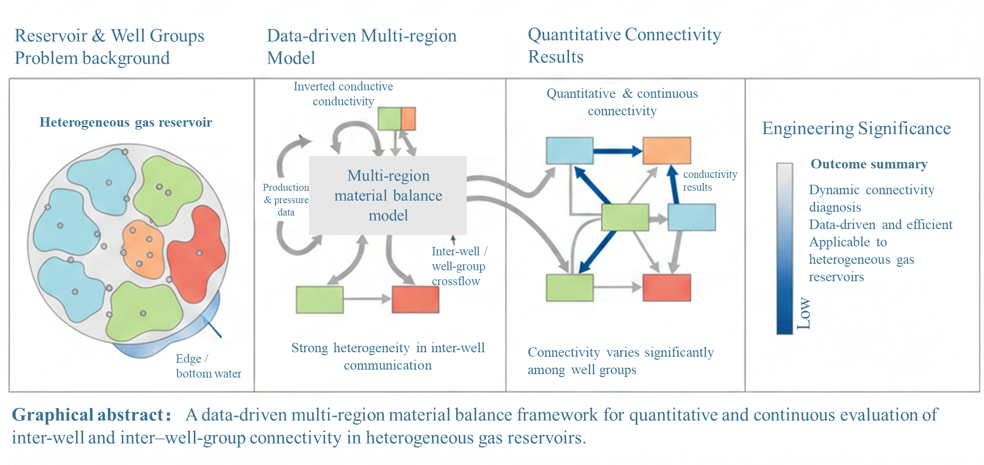
Carbonate gas reservoirs are often characterized by strong heterogeneity, complex inter-well connectivity, extensive edge or bottom water, and unbalanced production, challenges that are also common in many heterogeneous gas reservoirs with intricate storage and flow behavior. To address these issues within a unified, data-driven framework, this study develops a multi-block material balance model that accounts for inter-block flow and aquifer influx, and is applicable to a wide range of reservoir types. The model incorporates inter-well and well-group conductive connectivity together with pseudo–steady-state aquifer support. The governing equations are solved using a Newton–Raphson scheme, while particle swarm optimization is employed to estimate formation pressures, inter-well connectivity, and effective aquifer volumes. An unbalanced exploitation factor, UEF, is introduced to quantify production imbalance and to guide development optimization. Validation using a synthetic reservoir model demonstrates that the approach accurately reproduces pressure evolution, crossflow behavior, and water influx. Application to a representative case (the Longwangmiao) field further confirms its robustness under highly heterogeneous conditions, achieving a 12.9% reduction in UEF through optimized production allocation.Graphic Abstract
Keywords
Naturally fractured carbonate gas reservoirs are typically characterized by strong heterogeneity, widespread distribution of edge/bottom water, and complex connectivity between gas wells or well groups. In carbonate gas reservoirs, heterogeneity is not only reflected in porosity and permeability variations but also arises from the irregular spatial distribution of fractures and vugs. These features result in complex and anisotropic flow paths, making inter-well connectivity highly variable and non-intuitive. Due to the differences in the gas wells’ production time and production rate, the non-uniform water influx in the gas reservoir is serious, and the formation pressure distribution and production performance are becoming more and more complex. Influenced by the uneven pressure distribution, water tends to preferentially encroach through zones with higher permeability, leading to early water breakthrough in specific wells, while other areas are abundant in gas. To improve the gas recovery, it is essential to determine the distribution of preferential channels among the gas wells/well groups and aquifer, and the accurate evaluation of inter-well/well group connective conductivity and aquifer volume plays a crucial role in determining the gas reservoir scale and optimizing well pattern and locations. Additionally, to mitigate the formation pressure differences between inter-well/well group and severe non-uniform water influx that are generated from unbalanced development in the gas reservoir, it is essential to balance the inter-well formation pressure and reduce the influences of water influx by optimizing the production schemes, which can provide a solid foundation for formulating development policies.
The inter-well connectivity evaluation methods, including static and dynamic approaches, are summarized in Table 1.
Table 1: Comparison of static and dynamic methods for evaluating inter-well connectivity.
| Method Type | Representative Approaches | Advantages | Limitations |
|---|---|---|---|
| Static methods | Seismic interpretation; well logging correlation; sedimentary unit analysis [1,2,3]. | Geological background; qualitative connectivity; low cost | Non-quantitative; interpretation-dependent; no dynamic response |
| Dynamic methods | Production data analysis; pressure transient analysis (PTA); interference testing; rate transient analysis (RTA); multi-region material balance equation (MBE); numerical simulation [4,5,6,7]. | Quantitative connectivity reflects flow communication; considers aquifer effects | Data-intensive; higher computational cost |
| Hybrid/semi-analytical approaches | Lumped multi-region MBE with inter-region flow; data-driven inversion. | Balanced efficiency and accuracy; suitable for well-group analysis | Assumption-dependent; limited spatial resolution |
As summarized in Table 1, static methods mainly provide qualitative geological insights, while dynamic methods focus on quantitative evaluation of flow communication based on reservoir performance. To balance computational efficiency and modeling accuracy, this study adopts a hybrid, multi-region material balance framework with inter-well/well-group connectivity, enabling quantitative connectivity assessment using readily available production and pressure data.
For gas reservoirs with edge/bottom water, the evaluation for aquifer volume and water influx rate is the basis of designing water-control measures and exploiting the gas reservoir efficiently [8,9]. Currently, the evaluation of aquifer volume can be mainly divided into three categories. The first method is geologic description, which uses seismic and logging data to determine the range and volume of the aquifer roughly. This method is quick and simple, but it cannot describe the aquifer accurately and quantitatively [10,11,12]. The second method is dynamic data analysis, and it combines MBE and gas reservoir dynamic data. This method is relatively accurate, while it relies on high-precision monitoring data [13,14,15]. The third method is numerical simulation, and it is conducted by establishing the geological model and inverting the aquifer volume and locations after the production history-matching. Although this method can accurately describe the aquifer, the process is complex and work-intensive [16,17,18].
Unbalanced exploitation of gas reservoirs may lead to insufficient gas reserves and earlier water influx, which then affects the long-term stability of the gas reservoir and the economic benefits [19,20,21]. Currently, to achieve the balanced development of gas reservoirs, some scholars have suggested that for heterogeneous gas reservoirs with complex storage and permeable spaces, based on the fine reservoir description, the well spacing density should be reasonably increased to improve the swept coefficient of pressure drop, and the pressure decline rate should be enhanced through the measures of hydraulic fracturing and pressurization [22]. For gas reservoirs with complex gas and water distribution, based on the characteristics of the aquifer distribution and the contact of gas-water phases, the well types, locations, production rates and water drainage measures should be reasonably deployed, which can ensure the uniform advancement of the water-gas front, the improvement of water influx efficiency, and the reduction of residual gas [23,24,25]. However, currently, the traditional gas reservoir engineering and numerical simulation models are always used for the optimization of gas well production rate, which has lower precision and adjustment efficiency, and poor feasibility [26,27,28]. In contrast to the limitations of these traditional approaches, reasonable production allocation and balanced development remain critical objectives in gas reservoir management, especially under water-drive conditions [26,28,29,30].
To address the issues in the above studies regarding the efficient and accurate evaluation on the inter-wells/well groups connectivity and aquifer volume, and the optimization of gas well production rate for balanced development, the inter-well/well groups connective conductivity is introduced to consider the crossflow, and the aquifer volume and water influx index are used to evaluate the aquifer quantitatively and dynamic water influx. Through the modification of the MBE with a supplement for edge/bottom water-drive gas reservoir, a mathematical model for calculating the production performance in a gas reservoir with multiple well groups is presented. In combination with the PSO algorithm, the formation pressure is matched, and then the estimated ultimate recovery (EUR), inter-well/well groups conductivity and the aquifer volume, water influx factor are inverted [31]. The accuracy of the model is validated through comparisons with some synthetic gas reservoir numerical simulation models and the practical applications in the LWM gas reservoirs. In addition, through the introduction of UEF, and the combination of the presented model, the operating rate of gas wells in the next year is optimized, which can provide some guidance for the adjustment of technical polices and production schemes.
According to the heterogeneity of the gas reservoir and the distributions of well locations, the gas reservoir is divided into n blocks that are independent and are not closed, in which one region usually contains one or more gas wells (Fig. 1). The assumptions include:
- (1)The reservoir and aquifer pressure for each block is the same before the gas reservoir is put into production, and it has uniform pressure.
- (2)When the production gas reservoir is put into production, due to the differences in the gas reserves, cumulative gas production and water influx rate for each block, the pressure difference occurs among the blocks, which leads to the gas supplement between the blocks;
- (3)The compressibility of rock and connate water is considered;
- (4)The aquifer for each block is independent, and the water influxes into the reservoir in the pseudo steady state.
In this context, ‘pseudo steady state’ indicates that although the aquifer pressure decreases with time, the internal pressure profile maintains a quasi-stable shape. This assumption, commonly used in the Fetkovich model, enables the water influx to be calculated as a function of the block pressure without explicitly solving spatial flow equations.
According to the above assumptions, the MBE with supplement in edge/bottom water-drive gas reservoir for each block can be presented, which is shown in Eq. (1):
For zones 1 and n, the expression is different from Eq. (1), which can be expressed as Eq. (3) and Eq. (4), respectively.
In Eqs. (1)–(4), pi is the gas reservoir initial pressure, MPa; pj is the formation pressure of zone j at a certain moment, MPa; Gj and Gpj are the gas initial in place for zone j and the cumulative gas production at a certain moment, 108 m3; zi and zj are the gas correction factors in the initial condition and for the zone j at a certain moment, respectively; Ce is the compressibility coefficient for the gas reservoir rock and connate water, MPa−1; Δpj is the pressure drop in zone j at a certain moment, MPa; Gjk and Gmj are the cumulative gas flow rate from zone j to zone k and from zone m to zone j at a certain moment, respectively, 108 m3. Wej is the cumulative water influx at a given moment in zone j. Wpj is the cumulative water production at a given moment in zone j, m3. It is worthwhile to note that since the number of blocks that are connected to zone j is generally less than n, the crossflow rate between some blocks and zone j is indeed 0.
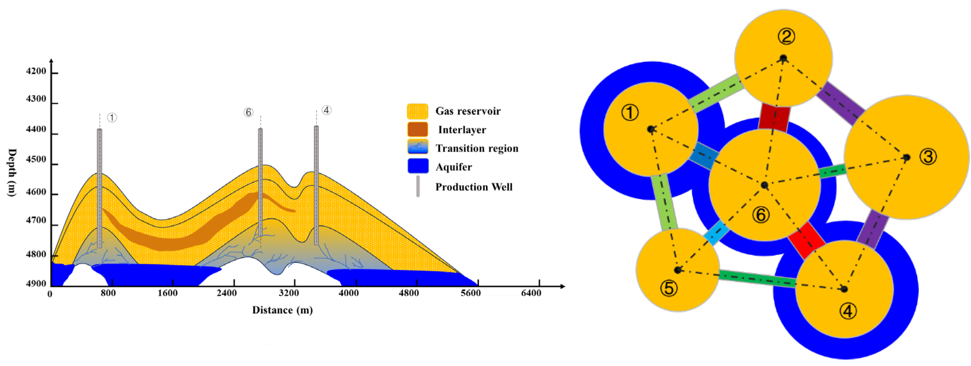
Figure 1: Schematic of gas reservoir with edge/bottom aquifer (left) and conceptual model (right).
When the gas reserve is known, the MBE with supplement, as shown in Eqs. (1)–(4), which are the functions of formation pressure in each zone, then Eqs. (1)–(4) can be rewritten as:
2.2.1 Inter-Wells/Well Groups Crossflow
For the calculation of gas crossflow rate from zone j to zone k in Eq. (1) at a certain time, it is assumed to conform to Darcy’s law, and the formula is:
In Eq. (8), Bg is the gas volume factor, μg is the gas viscosity, mPa·s; α is a constant, 0.0864; mj and mk are the pseudo-pressure for zones j and k, respectively, and the formula is:
To reflect the magnitude of connectivity between zones j and k directly, the concept of connectivity conductivity is introduced, which is defined as:
According to Eq. (10), Tjk represents the connective conductivity between zones j and k, with units of mD·m. It is a function of the average inter-zonal permeability (kjk), contact area (Ajk), and distance between zones (Ljk), and is independent of fluid properties. This means Tjk reflects only the static geological and geometrical characteristics of the gas reservoir. In this study, connective conductivity is introduced as a practical parameter to quantify the flow capacity between different zones or well groups in water-drive gas reservoirs. As we all know, in the traditional numerical simulation, the transmissibility quantifies the fluid flow capacity between two adjacent grid cells, which is the function of formation permeability, fluid mobility, and the geometric configuration/contact relationship of the grid cells. Compared with the transmissibility among grids, connective conductivity is fluid-independent and avoids reliance on precise geometric or petrophysical inputs that are often difficult to obtain in practice. By using this simplified representative formulation, the model reduces uncertainty associated with direct parameter estimation and provides a robust means of describing inter-well connectivity.
Substituting Eq. (10) into Eq. (8) yields:
In Eq. (8), T is the temperature of gas reservoir, K; Psc and Tsc are the pressure and temperature in the standard condition, 0.101 MPa and 298.15 K, respectively.
At the time of t + Δt, the cumulative gas crossflow rate from zone j to zone k is solved by the successive iteration, and the equations are shown as follows:
Substituting Eq. (11) into Eq. (12) yields:
2.2.2 Water Influx Calculation
The models for water influx calculation mainly include Fetkovich, Carter-Tracy and Van Everdingen-Hurst [32,33,34]. The Fetkovich model can be used for radial, linear and spherical water-influx, which is simple and has a wide range of applicability; therefore, it is adopted in this study to calculate the water influx.
It is assumed that the water influx process is pseudo steady-state flow, and the total compressibility of the aquifer is constant. The cumulative water influx is calculated by the following formula:
Eq. (14) can be transformed into:
The maximum water influx Wei can be defined as:
Substituting Eq. (16) into Eq. (15) yields:
The water influx rate can be obtained by differentiating both sides of Eq. (17), and after transformation, it can be written as:
Integrate the third and fourth items about the variables
In Eq. (19), it is assumed that the formation pressure on the inner boundary is constant. However, in fact, this pressure changes continually as the increase of gas production.
Therefore, actually, it is assumed that the boundary pressure within the aquifer is equal to the gas reservoir pressure; then according to the production period of the gas reservoir, the changes of the boundary pressure within the aquifer can be divided into n stages. The water influx rate can be calculated for each state sequentially. Based on the above principle, the amount of water influx rate in the nth period is calculated as:
Then
2.2.3 Newton-Raphson Iteration
To solve the formation pressure for each block, the gas crossflow rate between blocks and the water influx rate at every moment are considered. The Newton-Raphson non-linear iterative method is introduced to solve the presented model, as shown in Eqs. (5)–(7), which is expressed as follows:
In Eq. (23), l is the number of iterations. According to Eq. (13), the non-linear iterative matrix can be given:
In the Jacobi matrix on the left side of Eq. (24), the formula for each variable is written as:
If zones j and k (or m and j) are adjacent to each other, then there is connectivity between these two zones, which is calculated as:
If zones j and k (or m and j) are not adjacent to each other, they are not connected, which can be calculated as:
According to Eqs. (25)–(27), it can be seen that the Jacobi matrix is strictly diagonal dominant and symmetric, which has better convergence and stability. Thus the formation pressure solution for each zone at each time step can be obtained accurately.
2.3 Production History Match and Optimization
2.3.1 Production History Match and Parameters Inversion
Through the utilization of the solution process presented in Section 2.2, the developed MBE with supplement for multiple wells/well groups in edge/bottom water drive gas reservoir can be solved numerically, and the formation pressure for each block at different time steps can be obtained. These calculation results mainly depend on the reserve of the block, the inter-well conductivity and the aquifer volume. In practice, the inversion for these parameters can be realized by optimizing and adjusting these parameters to make the best match between the calculated formation pressure and the actual monitoring values. For this purpose, the following minimization target function can be defined:
For the optimization issue shown in Eq. (28), the PSO is used to deal with it, which is a stochastic optimization method. It is assumed that a possible solution is a particle, then each particle can be regarded as an individual in the D-dimensional search space. The current position of the particle is the candidate solution for the optimization issue. The velocity and position of each particle are updated through the continuous iterative search and computation until an optimal solution that satisfies the termination condition is obtained. The primary parameters, the particles and max iterations are set to be 24 and 2000, respectively. The learning factors include the cognitive learning factor and social learning factor, and are set to be 2.1. Inertia weights control the global and local velocity, are set to be 0.9 and 0.6, respectively.
To quantitatively evaluate the balanced degree of well production for a gas reservoir with edge/bottom water, the unbalanced exploitation factor (UEF) Ef is defined, which is used to reflect the difference between the formation pressure for each well group and the average gas reservoir pressure. The smaller the UEF is, the more balanced the degree of reservoir is. Indeed, this factor is the function of the production rate for each well group, and the expression is shown in Eq. (29):
Based on the presented production history match and parameters inversion method in Section 2.3.1 and the proposed production optimization method in Section 2.3.2, a flowchart for gas formation pressure match, parameter inversion, and production optimization for each block was established, as shown in Fig. 2.
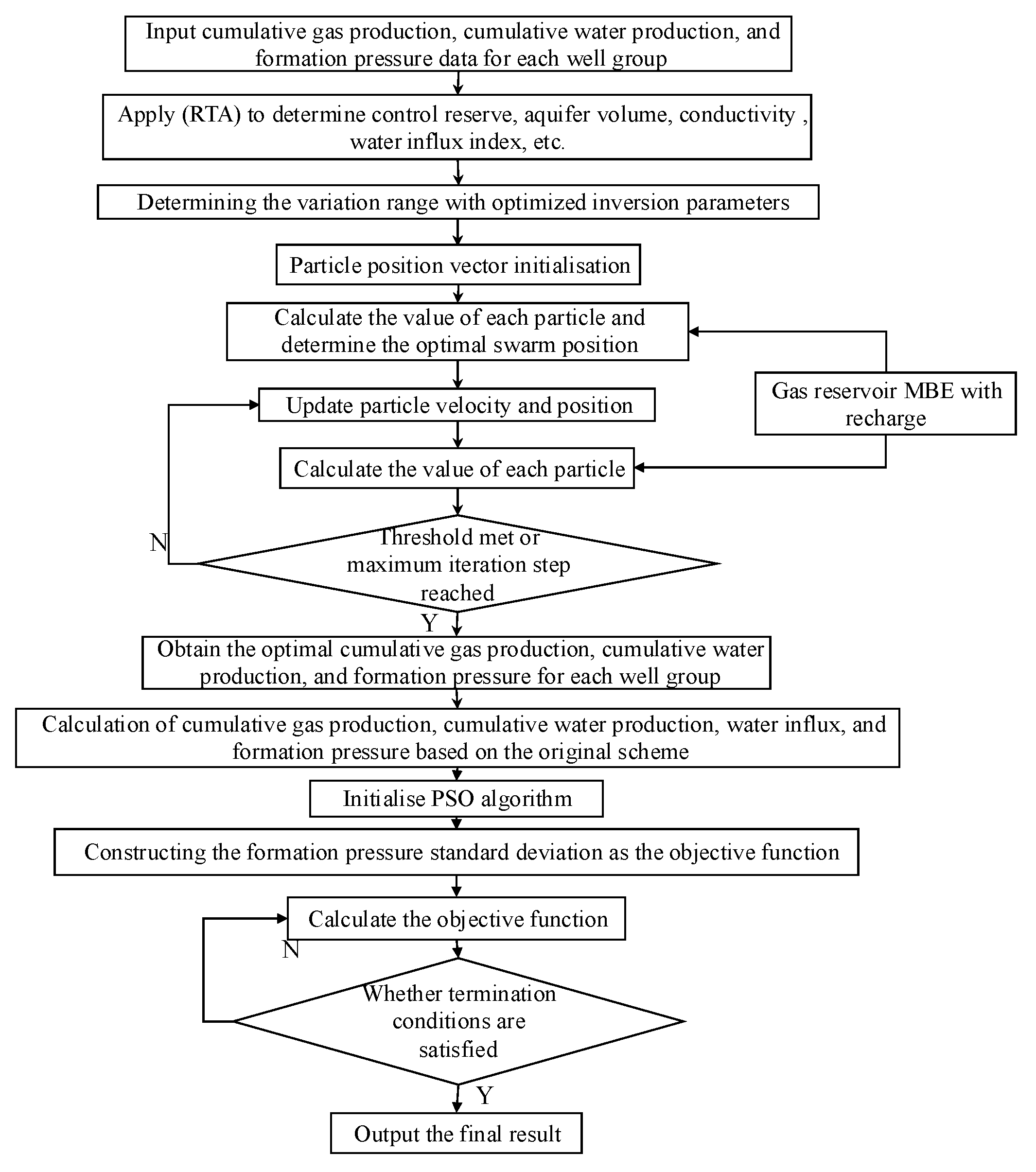
Figure 2: Flowchart of formation pressure matching and inversion calculation for model parameters.
To verify the accuracy and the validity of the model established in Section 2, a numerical simulation model for an edge/bottom water gas reservoir with two gas wells was developed, as shown in Fig. 3. The location of wells P1 and P2 is defined as Zones 1 and 2, respectively. For the base case, the dominant area and gas reserves are assumed to be identical for both wells. An intermediate zone with different permeability from the two blocks is included to characterize seepage channels with varying conductivities. The specific model parameters are given in Table 2, and the relative permeability curves are shown in Fig. 4:
Table 2: Parameters of the numerical simulation model.
| Parameters | Value | Parameters | Value |
|---|---|---|---|
| Grid size/m | 10 × 10 × 10 | Zone 1/Zone 2 gas reservoir permeability/mD | 100 |
| Grid number | 180 × 80 × 4 | Flowing channel permeability/mD | 0.01 |
| Formation temperature/°C | 140.2 | Flowing channel size/m | 20 × 800 × 40 |
| Top depth of gas reservoir/m | 4300 | Initial formation pressure/MPa | 75.8 |
| Porosity/% | 15 | Gas well production rate/(104 m3/d) | 10(P1), 20(P2) |
| Total compressibility/MPa−1 | 5.943 × 10⁻⁵ | Production time/d | 1500 |
| Zone 1/Zone 2 gas reserves/108 m3 | 12.1 | Connective Conductivity/(mD·m) | 10 |
| Zone 1/Zone 2 aquifer volume/108 m3 | 10 | Zone 1/Zone 2 water influx index/(m3/d/MPa) | 10,000 |
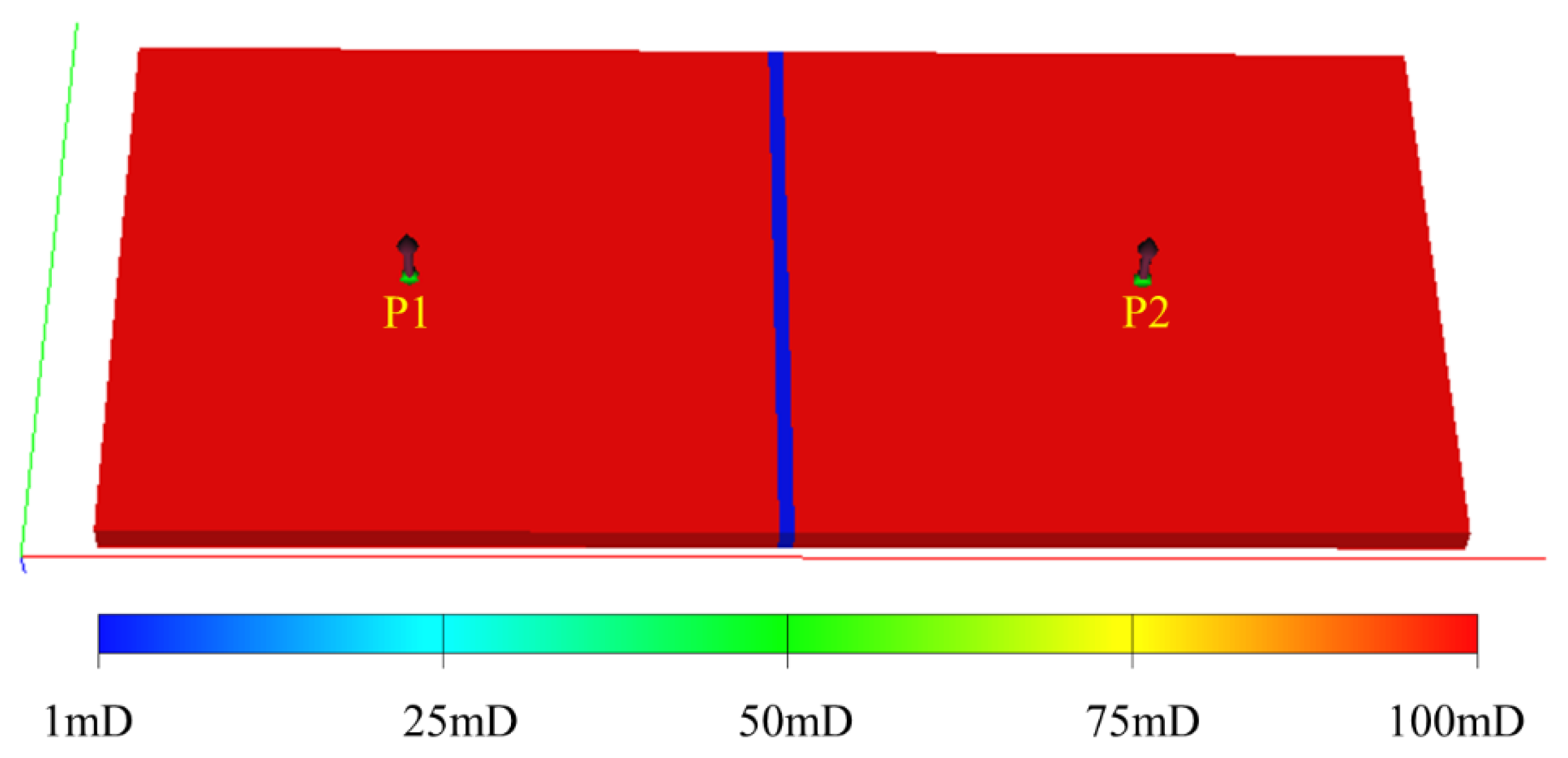
Figure 3: Permeability map for the synthetic gas reservoir numerical simulation model.
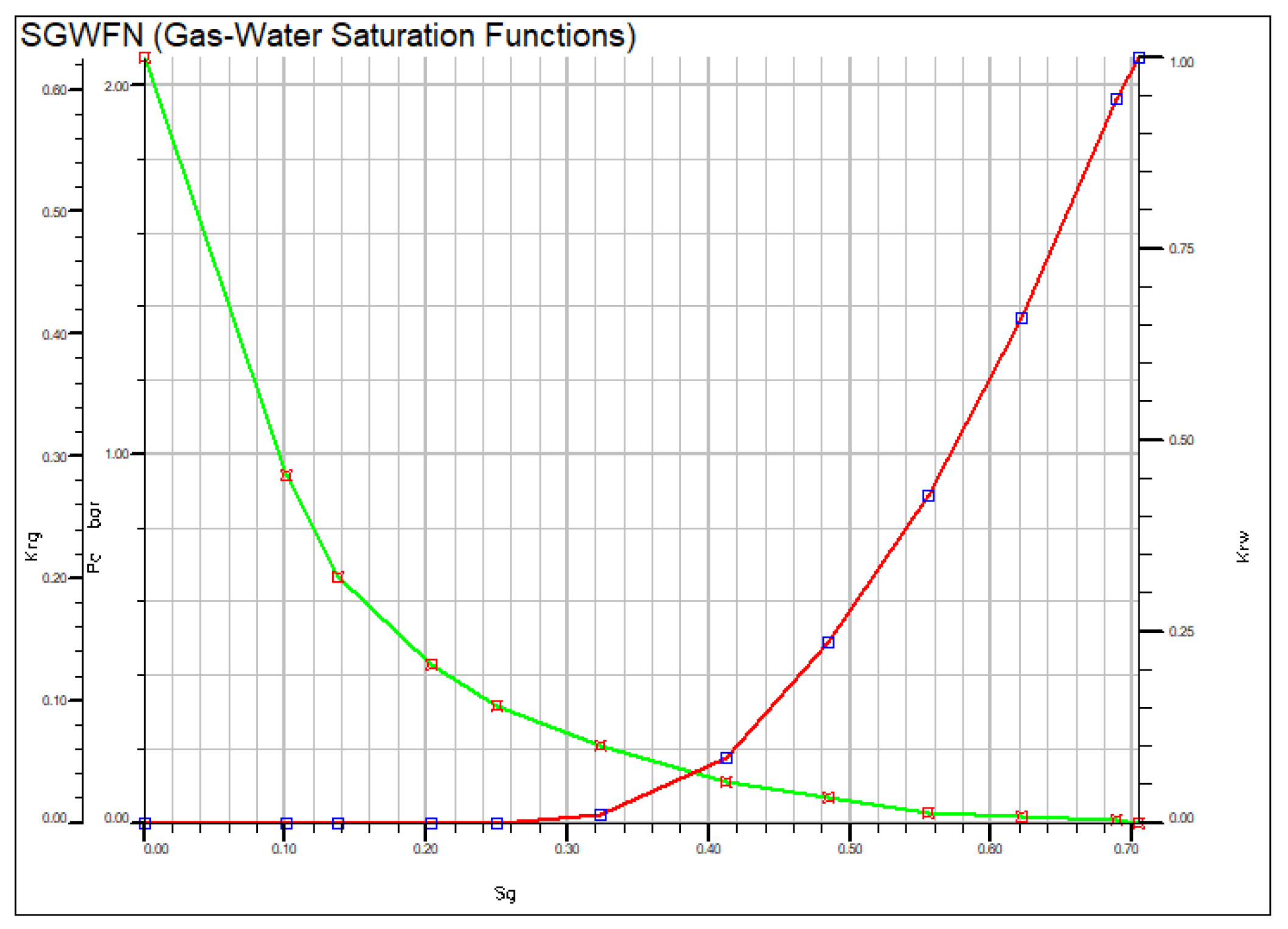
Figure 4: Relative permeability functions corresponding to the numerical model parameters in Table 1.
According to the above-presented numerical simulation model, the cumulative gas production of P1 and P2 wells, the formation pressure of each block and cumulative water influx can be obtained. The model parameters, such as gas reserves, connectivity conductivity, aquifer volume, water influx index and the cumulative gas and water production rate are inputted into the model to calculate the formation pressure of these two blocks, inter-wells/well groups crossflow rate, and the total cumulative water influx rate into the gas reservoir were obtained, which are compared with the numerical simulation results (Fig. 5b). It can be seen from this figure that with the presented model in this study, the formation pressure for each block, inter-well/well groups crossflow rate and cumulative water influx can be predicted accurately. The results show that the average errors between formation pressure, inter-wells/well groups crossflow rate and cumulative water influx rate, and the numerical simulation values are 0.01%, 6.41% and 6.75%, respectively, which are less than 10%. As the formation pressure is the main parameter that is matched with this proposed model, the average errors between formation pressure and numerical simulation value are the smallest. Actually, the inter-wells/well groups crossflow and water influx are unsteady state; however, in this article, to simplify the calculation, the inter-wells/well groups crossflow rate and water influx rate are calculated with the pseudo-steady state equations, which causes the errors with the numerical simulation values to be larger than the formation pressure. Generally, these differences are relatively small, which conforms to the needs of applications, thus verifying the accuracy and validity of the model.
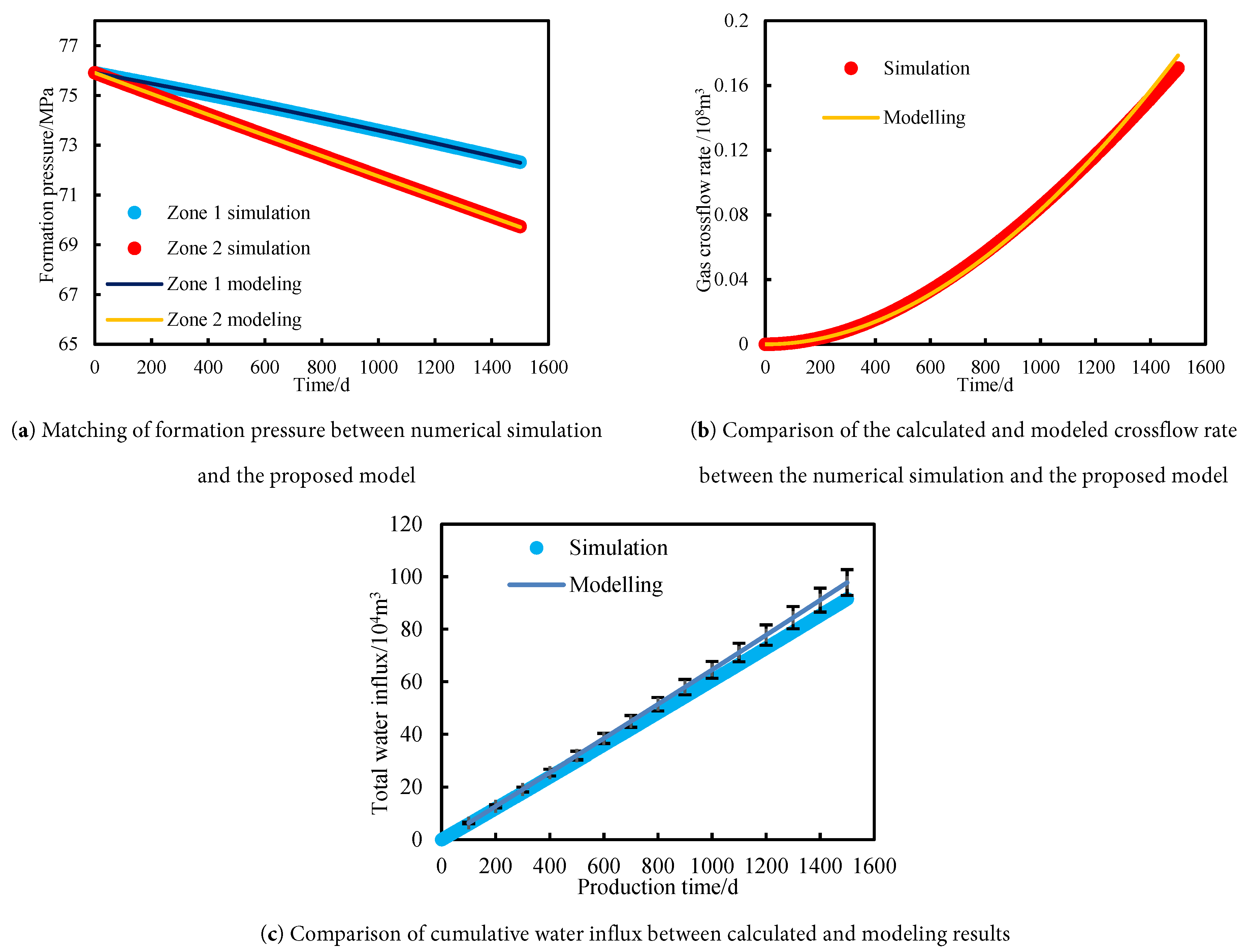
Figure 5: Matching of formation pressure and comparison of gas crossflow rate and cumulative water influx.
To show the robustness of the proposed model under varying reservoir and production conditions, it is essential to conduct the sensitivity analysis of the varied production rate, Inter-well/well groups conductivity and aquifer volume on the production performance. The following section mainly shows the influences of these three parameters on the matching accuracy and the prediction errors.
Adjustments of the gas wells’ production rate can lead to changes in reservoir pressure, thus the direction and the rate of gas flow, and the water influx rate between the target well and surrounding wells are influenced. To test the reliability of the model under different gas well production rates, two sets of experimental cases were developed. For case 1, the production rate of well P1 is 10 × 104 m3/d during the period 1~181 d, and the rate changes to 30 × 104 m3/d from the 182nd day. For case 2, the well P1 is shut during the period 1~181 d, and the rate changes to 40 × 104 m3/d from the 182nd day. In these two cases, the gas production rate is constant. According to the above two cases, firstly, numerical simulation was used to obtain the gas well production performance and pressure data. These data were input into the established model to calculate formation pressure, inter-wells/well groups crossflow rate and cumulative water influx rate. The comparisons between numerical simulation and calculated results are shown in Fig. 6.
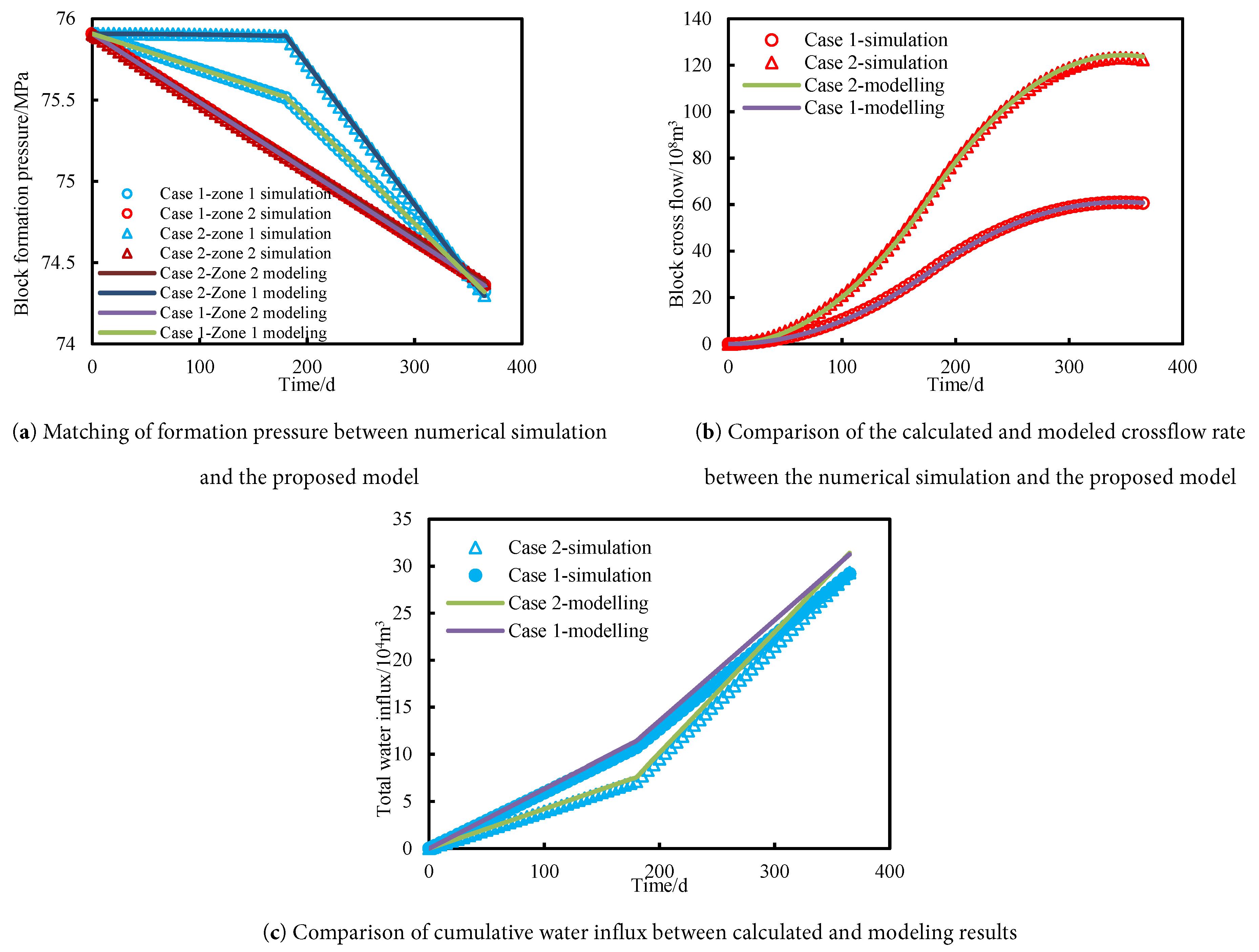
Figure 6: Matching of formation pressure and comparison of gas crossflow rate and cumulative water influx under different gas well production rates. The circles and triangles represent the data obtained from numerical simulation, and the solid lines represent the results that are calculated with the proposed model.
It can be seen from Fig. 6a that the formation pressures in zones 1 and 2 under different production rates are matched and predicted very well with the presented model. The deviations for formation pressure, gas crossflow rate, and cumulative water influx in these two cases are 0.004%/0.003%, 4.5%/4.2%, and 6.6%/6.2%, respectively. All these values are lower than 7%, which verifies the accuracy of the model. Through the observation of Fig. 6b, for case 2, due to the shut-off of well P1 in the period of 1~181 d, the formation pressure for zone 1 is higher than zone 2, which makes the rise of cumulative gas crossflow rate from zone 1 to zone 2. While on the 182nd day, well P1 begins to produce with the rate of 40 × 104 m3/d, after about 180 days’ production, the formation pressure of zone 1 is lower than zone 2, and the direction of gas crossflow reverses. The gas in Zone 2 starts to flow to Zone 1, which indicates the gas crossflow rate from Zone 2 to 1 is negative, and then the cumulative gas crossflow rate from Zone 1 to 2 reduces gradually. However, compared to the model that does not consider water influx [35], due to the supplement of water influx, the formation pressure of these two zones for different gas production rates is almost identical with each other. In addition, it can be seen from Fig. 6c that due to the shut-in of well P1 in the early stage for case 2, the rise of the cumulative water influx rate is significantly lower than case 1. However, because the cumulative gas production for these two cases is nearly identical, it results in the same cumulative water influx at the end of the period for these two cases.
4.2 Inter-Well/Well Groups Conductivity
Due to reservoir heterogeneity, the inverted conductive conductivity may vary significantly among different well groups within a given gas reservoir. To investigate the applicability of the model under different connectivity conditions, the inter-well or inter–well-group permeability was adjusted to simulate reservoir production performance over a range of conductivity values. Therefore, two cases are designed with inter-well/well groups permeabilities of 0.05 mD and 0.005 mD, and the corresponding conductivities are 50 mD·m and 5 mD·m, respectively. The rest of the parameters are kept constant with the base case. Numerical simulation is used to obtain the gas and water production rate. The proposed model is applied to match the production data and calculate the inter-block gas crossflow rate and cumulative water influx rate, which are shown in Fig. 7.
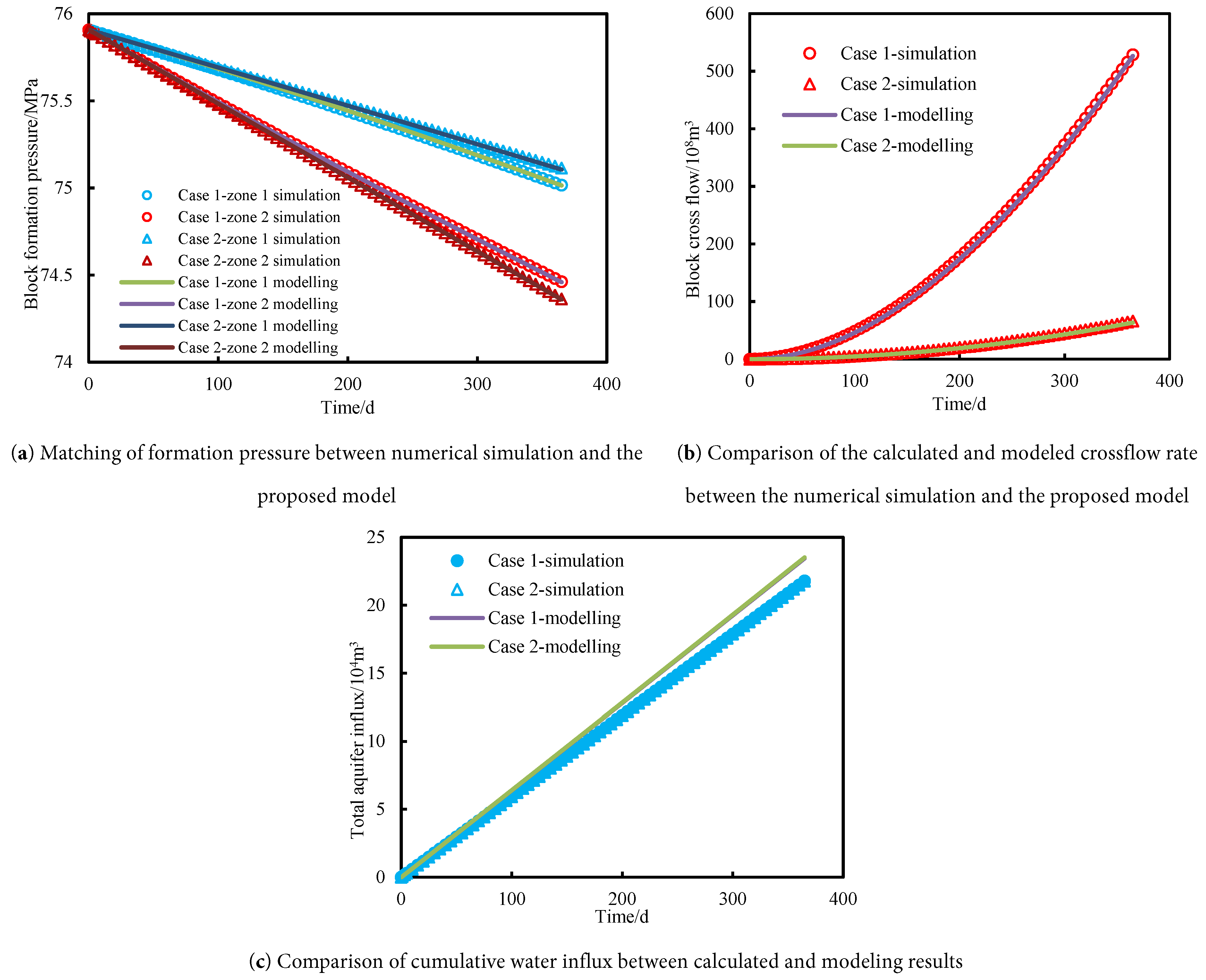
Figure 7: Matching of formation pressure and comparison of gas crossflow rate and cumulative water influx under different inter-well groups connective conductivity the circles and triangles represent the data obtained from numerical simulation, and the solid lines represent the results that are calculated with the proposed model.
It can be seen from Fig. 7 that the model proposed in this paper can match the formation pressure for these two cases very well, and the relative error is less than 0.01%. There is good conformity between the calculated inter-block gas crossflow rate, cumulative water influx and the values acquired from the numerical simulation, and the errors are 5.2%/8.3% and 7.5%/7.8%, respectively, which are relatively small and below 10%. These results confirm the accuracy of the model calculations. It can also be seen from this figure that when the inter-block permeability is low, the conductivity between zones 1 and 2 is relatively poor, which leads to a significant reduction of gas supplement from zone 1 to zone 2. Thus, the formation pressure in zone 1 for case 1 is much higher than in case 2, while the formation pressure in zone 2 is lower than in case 1. However, since the cumulative gas production rate remains constant, the change in cumulative water influx is the same in these two schemes.
The heterogeneous distribution of the aquifer in the gas reservoir makes the aquifer volume for one well vary greatly. Thus, through the change of aquifer volume for each dominant area, two cases with different aquifer volumes are designed properly to explore the validity of the presented model at different aquifer volumes. In case 1, the aquifer volume for two zones is 1 × 10⁸ m3, and the aquifer multiplier is 23.4. In case 2, the aquifer volume for two zones is 0.1 × 10⁸ m3, and the aquifer multiplier is 2.34. According to the designed cases, the production data can be obtained from numerical simulation, and then the formation pressure, inter-block gas crossflow rate and cumulative water influx can be matched with the presented model, which are shown in Fig. 8.
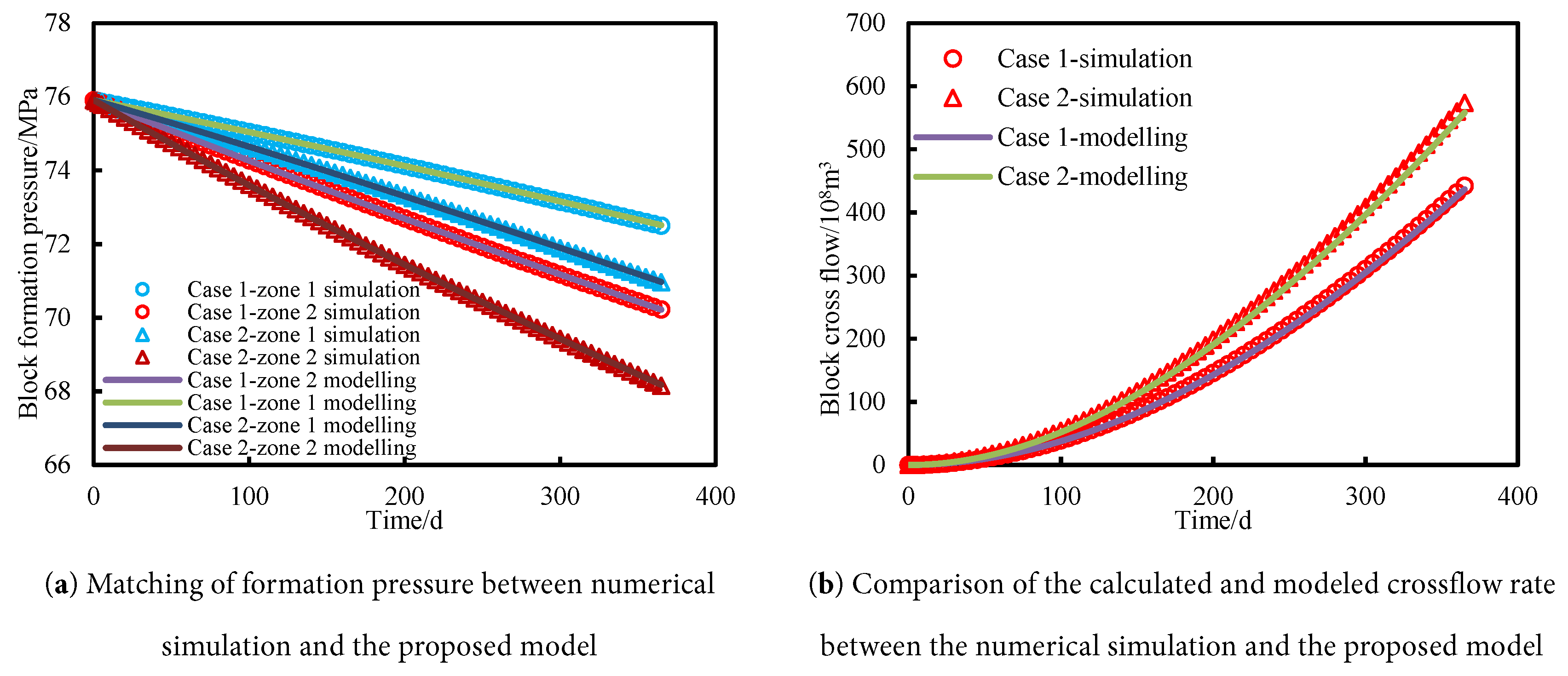
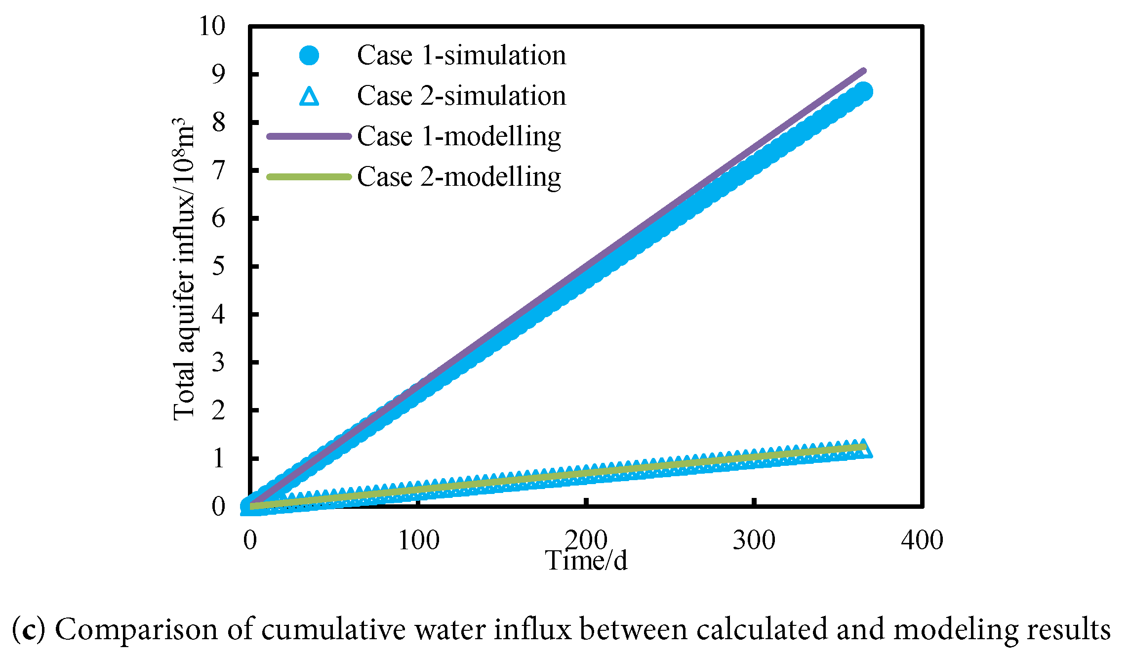
Figure 8: Matching of formation pressure and comparison of gas crossflow rate and cumulative water influx under different aquifer volumes. The circles and triangles represent the data obtained from numerical simulation, and the solid lines represent the results that are calculated with the proposed model.
Through the statistics of the matching results in Fig. 8, it can be found that it is found that the errors between the calculated formation pressure, inter-block crossflow rate and cumulative water influx and the numerical simulation results for these two blocks are 0.007%/0.014%, 4.95%/6.15%, and 5.38%/3.68%, respectively. All errors are below 7%, which also confirms the accuracy of the presented model. Through the observation of Fig. 8, due to the larger aquifer multiplier in case 1, the aquifer supplement is more sufficient, which makes the formation pressure and cumulative water influx of the gas reservoir in zones 1/2 in case 1 significantly higher than that in case 2. In addition, the sufficient supplement of water in case 1 reduces the pressure difference between Zone 1 and 2, which makes the inter-block cumulative gas crossflow rate of case 1 significantly lower than the values in case 2.
5.1 Evaluation of Inter-Well Groups Connectivity and Aquifer Volume
For the LWM gas reservoir in the Moxi gas field, there are three types of storage and seepage bodies: pores, fractures and vugs, which have serious heterogeneity. There are large differences in the drilled gas formation properties for each well/well group, which have the characteristics of connectivity and gas supplement among the beaches. In this study, a typical block is taken as an example. According to the geological and dynamic recognition, this reservoir with 18 gas wells is divided into 7 well groups (Fig. 9). In this gas reservoir, well groups G2 and G6 have an edge/bottom aquifer, which leads to the water production of gas wells in these two groups. According to the locations for each well group, the connection table can be determined, which is shown in Table 2. Through the utilization of the following material balance equation (FMB), rate transient analysis, the initial gas reserve for each well group can be acquired. The original gas reserve values in Table 3 were estimated using traditional rate transient analysis methods, such as FMB, Blasingame, and Agrawal-Gardner, based on production rate and wellhead pressure data. However, these methods do not consider inter-well connectivity or water-drive effects, which may reduce accuracy. In contrast, the inverted reserves were obtained using the proposed multi-block material balance model, which incorporates both inter-well flow and aquifer support, offering a more reliable estimate under complex reservoir conditions. Eq. (8) is used to calculate the initial inter-well groups conductivity, and the aquifer multiplier and water influx rate are obtained from numerical simulation and MBE.
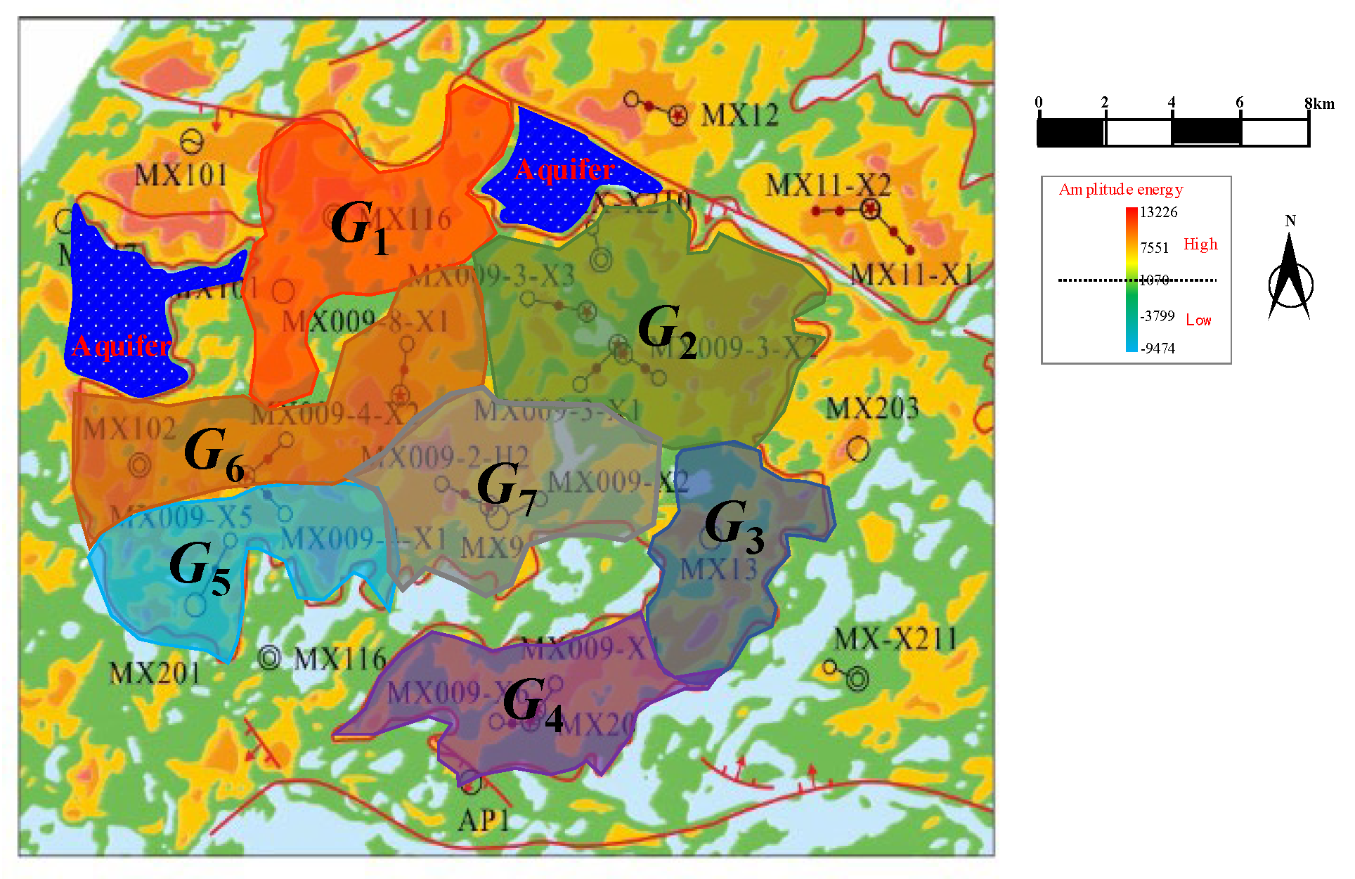
Figure 9: Schematic of divided well groups in LWM gas reservoirs.
Table 3: Parameters and connections of well groups within the well block.
| Well Group | Wells | Gas Reserves/108 m3 | Connected Well Group |
|---|---|---|---|
| G1 | 2 | 43.0 | G2, G6 |
| G2 | 3 | 104.4 | G1, G3, G6, G7 |
| G3 | 1 | 66.1 | G2, G4, G7 |
| G4 | 2 | 177.8 | G3, G5, G7 |
| G5 | 4 | 211.2 | G4, G6, G7 |
| G6 | 3 | 152.1 | G1, G2, G5, G7 |
| G7 | 3 | 122.0 | G2, G3, G4, G5, G6 |
With the established model in this paper, the formation pressure for each well group was matched (Fig. 10). At the same time, the proposed method for formation pressure matching and parameter inversion (Fig. 2) was applied to obtain the inter-well groups conductivity, gas reserves in the dominant area, aquifer volume, and water influx rate. The results are shown in Table 4. It can be seen from Fig. 10 that there is a good consistency between the calculated results and actual values, which indicates that the matched model is highly reliable. In Table 4, it can be found that the differences between the initial gas reserve and the inverse gas reserve are small. The two well groups (G2 and G6) with edge/bottom water have small aquifer multipliers, which are below 0.1 and suggest an insufficient aquifer supplement. However, due to the existence of fractures and vugs, the edge/bottom water flows along the flow preferential seepage channels to the wells, and thus the water influx index is larger, which is larger than 4 × 10⁴ m3/MPa/d. By observing the inverse inter-well groups conductivity for each well group (Fig. 10), it can be found that the conductivity between well groups G2 and G7 is the highest, which is 297.2 mD·m. Then it is the conductivity between well groups G2 and G3, which is 222.4 mD·m. These results indicate that well group G2 (X9-3-X1, X9-3-X2, X9-3-X3) has better connectivity with well group G3 (X13) and well group G7 (X9, X9-2-H2, X9-X2). This conclusion is consistent with the results obtained from the well interference test in the literature [2], which further verifies the accuracy of the interpretation of the proposed model.
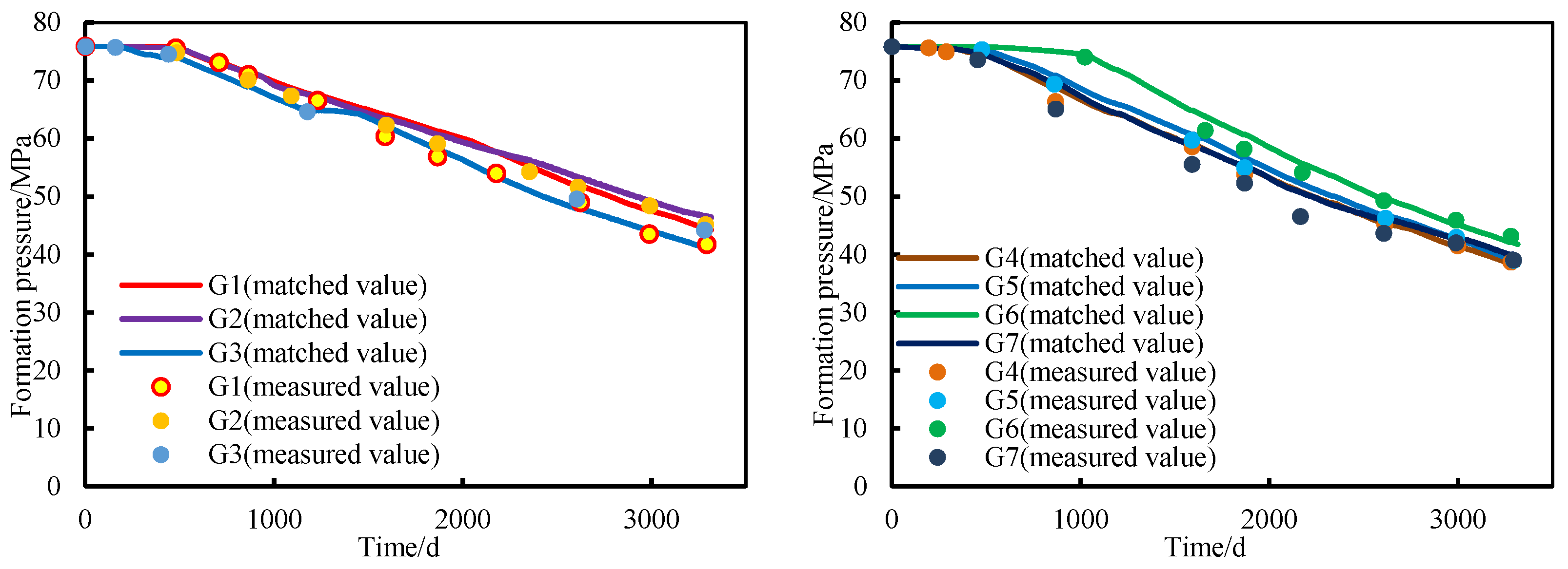
Figure 10: Formation pressure match for each well group.
Table 4: Statistics of inversion results for each well group.
| Well Group | Inversed gas Reserves/108 m3 | Deviation with Original Gas Reserve/% | Aquifer Multiples | Water Influx Index/(m3/d/MPa) |
|---|---|---|---|---|
| G1 | 38.91 | 9.5 | / | / |
| G2 | 97.07 | 7.0 | 0.09 | 41,023.0 |
| G3 | 63.80 | 3.5 | / | / |
| G4 | 160.02 | 10.0 | / | / |
| G5 | 194.67 | 7.8 | / | / |
| G6 | 136.89 | 10.0 | 0.1 | 68,284.0 |
| G7 | 111.19 | 8.9 | / | / |
5.2 Optimization of Gas Well Production
Based on the matched MBE model in Section 5.1, the balanced exploitation is taken as the target, and the optimization of the MX9 area in the LWM gas reservoir is carried out. The optimization period is one year (360 days), and the average daily gas production rate in the last month of the historical production period for each well group is used as the initial value for gas production prediction. For the water production wells/well groups, the water/gas ratio is assumed to remain unchanged, which was used to determine the water production rate. With consideration of the actual production conditions, the gas wells’ production rate varies from 0.5 to 2.0, and the number of optimization iterations is set to be 20. The variation of the gas reservoir UEF with the number of iterations is shown in Fig. 11. It can be seen from the Fig. 12 that as the number of iterations increases, the UEF decreases from the initial value of 5.9 to 5.1, which decreases by 12.9%. This indicates a significant improvement in the degree of balanced development for each well group in the gas reservoir.
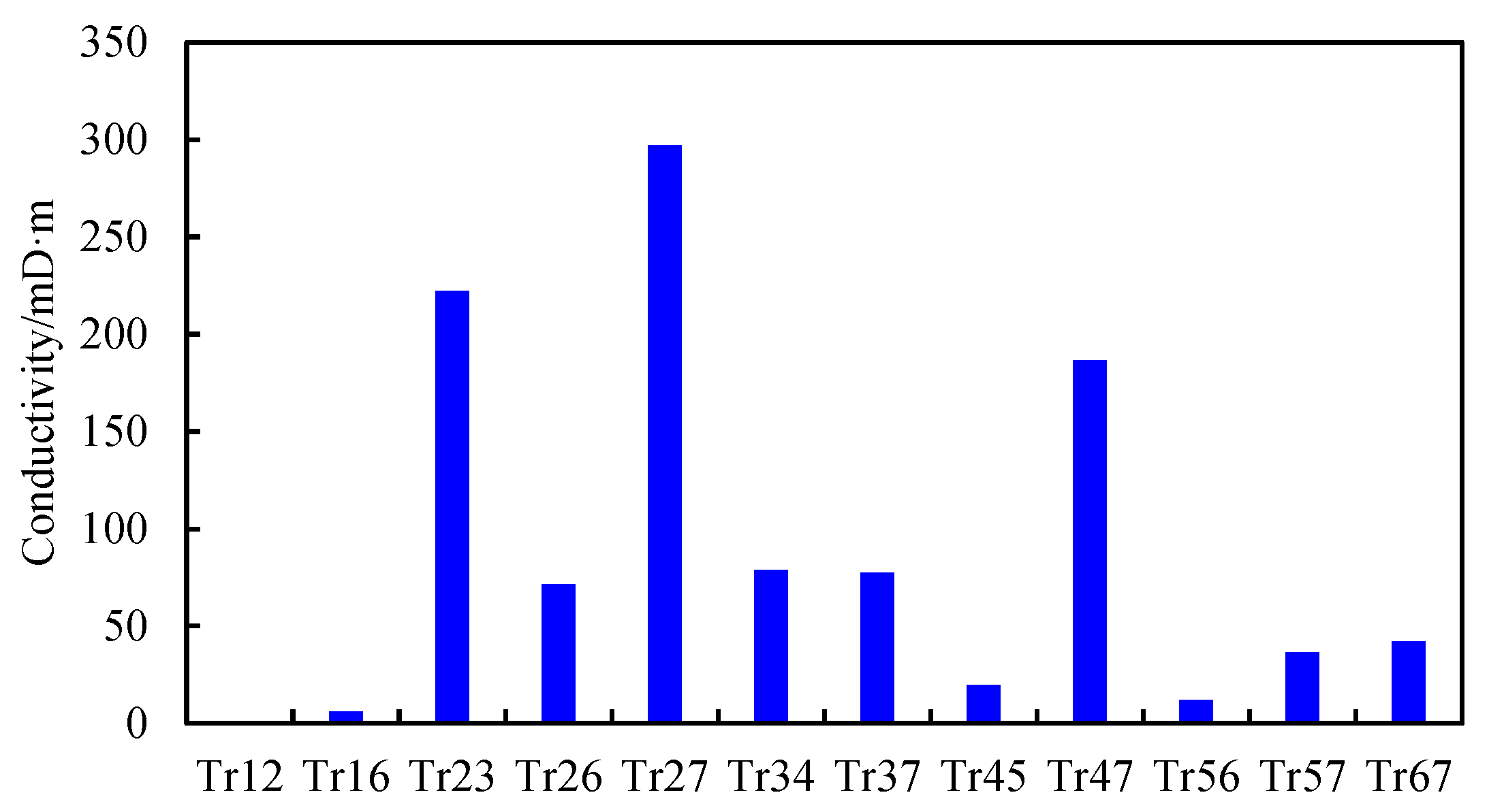
Figure 11: Comparison of inversion inter-well group conductivity results.
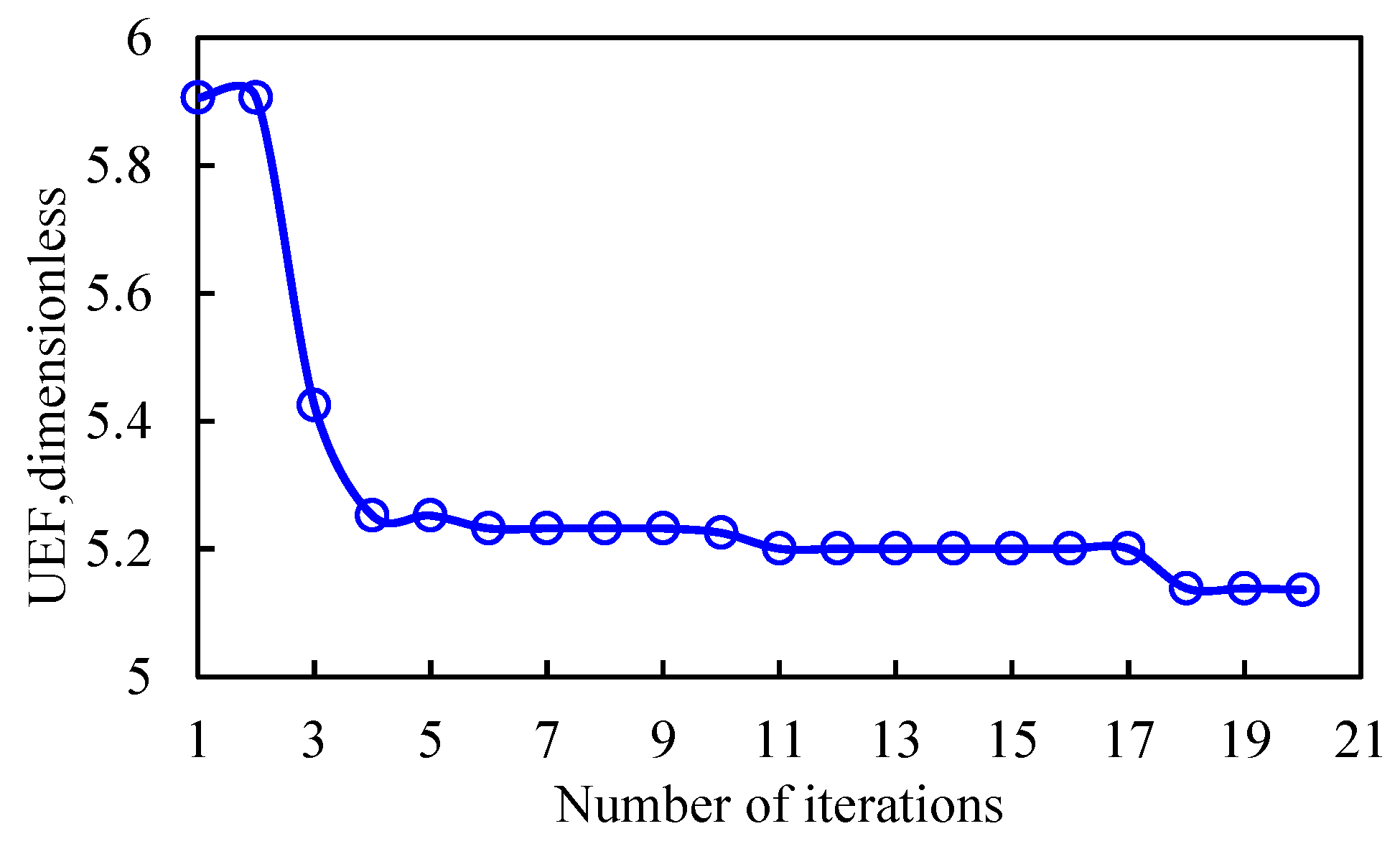
Figure 12: Variation of UFE with the iteration number.
Through the comprehensive analysis of the formation pressure curves for each well group before and after optimization (Fig. 13), it can be easily seen that the differences in formation pressure for each well group reduce significantly. Before the optimization, the well groups G1~G3 had smaller reserves and lower cumulative gas production. Additionally, there is higher reservoir pressure in these well groups due to the influence of water influx. In contrast, well groups G4, G5, and G7 have higher cumulative gas production rates and lower reservoir pressure. However, the formation pressure of well group G6 is significantly higher than well groups G4, G5, and G7 due to the influences of water influx. By optimizing the production rate of gas wells/groups, as shown in Fig. 14, the production rate for well groups G1~G3 is increased, which leads to a significant decrease of formation pressure in these well groups, and the reduction ranges from 0.9 to 2.6 MPa. However, this also results in the increase of water influx by 0.6 × 10⁴ m3. Meanwhile, by reducing the production rate for well groups G4–G7, the reservoir pressure in these groups increased by 0.7 to 2.1 MPa. At the same time, the reduced production leads to a decrease in the water influx by 0.7 × 10⁴ m3. From the aspect of the whole gas reservoir, the pressure of the gas reservoir is lifted and the cumulative water influx is reduced by 0.1 × 10⁴ m3, and the effects of balanced development are achieved, which can support the high and stable production of the gas reservoir in the long term.
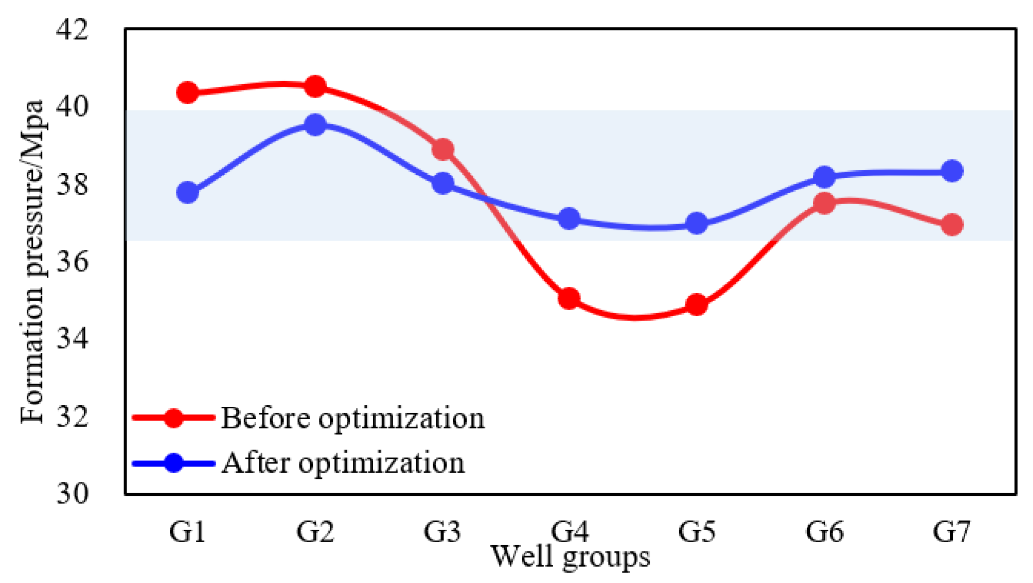
Figure 13: Comparison of formation pressure for each well group before and after optimization.
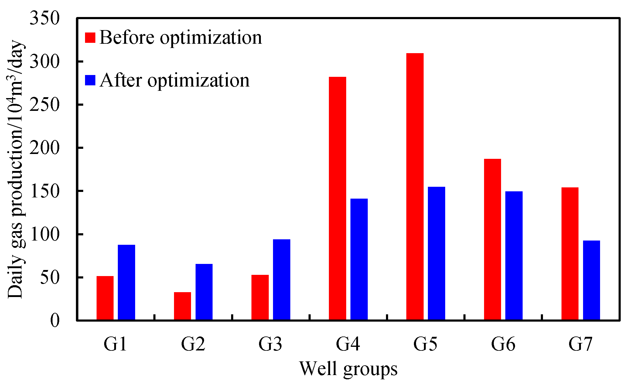
Figure 14: Comparison of daily gas production rate before and after optimization.
- (1)Based on the MBE model with supplement in edge/bottom water-drive gas reservoir, the concept of connectivity conductivity is introduced. The successive iteration method and the Fetkovich water influx model are used to solve this model. In combination with PSO, the formation pressure for each block is matched perfectly and the inter-well groups’ conductivity, aquifer volume, and water influx index are inverted accurately.
- (2)Synthetic cases for different production rates, inter-well group conductivity, and aquifer volume are designed properly. Through the comparisons with the formation pressure, cumulative water influx, and inter-well group gas crossflow rate that are acquired from numerical simulations, the errors between the presented model and the numerical simulations are less than 10%, which verifies the accuracy of the established model.
- (3)A gas block in the LWM gas reservoir is taken as an example; the proposed model is used for the matching of formation pressure and the inversion of conductivity, gas reserves, cumulative water influx, and water influx index. The results show that the formation pressure for each block can be matched well, and the inverse connectivity conductivity is consistent with the conclusions of the well interference test, which further proves the reliability of the proposed model.
- (4)The UEF is defined to represent the unbalanced development degree of a gas reservoir. After the optimization of the target gas reservoir in a year, the UEF decreases by 12.9%, and the formation pressure of some well groups is lifted by 0.7~2.1 MPa. In addition, the cumulative water influx rate decreases by 0.1 × 10⁴ m3, and the effects of balanced exploitation are achieved primarily, which provides some support for the high and stable production of the gas reservoir over a long period.
The connectivity evaluation framework proposed in this study provides a quantitative and continuous characterization of dynamic inter–well-group communication. The resulting conductivity values offer an effective basis for interpreting different flow communication mechanisms between well groups. At present, this study does not explicitly incorporate enhanced recovery strategies based on the connectivity analysis.
Future work may further integrate the proposed framework with targeted numerical simulation models to explore the potential implications of different connectivity conditions on recovery performance. In cases of weak connectivity, limited crossflow may indicate insufficient pressure support and incomplete drainage, which could be examined in future studies using localized stimulation or zonal control scenarios. For moderately connected well groups, partial pressure interference may warrant further investigation into production balancing strategies. Strongly connected well groups, which are more sensitive to pressure interference and aquifer response, may also be examined through coordinated, group-level production control scenarios. These aspects are beyond the scope of the present study and are suggested here only as possible directions for future research.
Acknowledgement:
Funding Statement: This work was supported by the National Natural Science Foundation of China (No. 52104018, 52274030), China National Petroleum Corporation (CNPC) Innovation Foundation (No. 2024DQ02-0303), and China National Petroleum Corporation (CNPC) 14th Five-Year Plan Major Strategic Scientific and Technological Project for Prospective and Fundamental Research (2024DJ86). All the supports are gratefully acknowledged.
Author Contributions: Conceptualization, Fankun Meng; methodology, investigation, software, validation, visualization, writing—original draft preparation, and writing—review and editing, Yuyang Liu; supervision, resources, and project administration, Xiaohua Liu; data curation, formal analysis, and validation, Chenlong Duan; investigation, visualization, and writing—review and editing, Yuhui Zhou. All authors reviewed and approved the final version of the manuscript.
Availability of Data and Materials: The data that support the findings of this study are available from the corresponding author upon reasonable request.
Ethics Approval: Not applicable.
Conflicts of Interest: The authors declare no conflicts of interest.
References
1. Li XZ , Guo ZH , Wan YJ , Liu XH , Zhang ML , Xie WR , et al. Geological characteristics and development strategies for Cambrian Longwangmiao Formation gas reservoir in Anyue gas field, Sichuan Basin, SW China. Pet Explor Dev. 2017; 44( 03): 398– 406. (In Chinese). doi:10.1016/S1876-3804(17)30049-6. [Google Scholar] [CrossRef]
2. Su YH , Li XZ , Wan YJ , Zhang L , Liu XH , Liu HI . Research on connectivity evaluation methods and application for dolomite reservoir with fracture-cave. Natural Gas Geoscience. 2017; 28( 08): 1219– 25. (In Chinese). [Google Scholar]
3. Wu KL , Li XF , Lu W , Xu BX , Hu SM . Application and derivation of material balance equation for abnormally pressured gas condensate reservoirs with gas recharge capacity and water influx. Earth Sci J China Univ Geosci. 2014; 39( 02): 210– 20. (In Chinese). [Google Scholar]
4. He YW , Cheng SQ , Qin JQ , Chai Z , Wang Y , Yu HY , et al. Interference testing model of multiply fractured horizontal well with multiple injection wells. J Pet Sci Eng. 2019; 176: 1106– 20. doi:10.1016/j.petrol.2019.02.025. [Google Scholar] [CrossRef]
5. Chu WC , Scott KD , Flumerfelt R , Chen C , Zuber MD . A new technique for quantifying pressure interference in fractured horizontal shale wells. SPE Reservoir Eval Eng. 2020; 23( 1): 143– 57. doi:10.2118/191407-PA. [Google Scholar] [CrossRef]
6. Hagoort J , Hoogstra R . Numerical solution of the material balance equations of compartmented gas reservoirs. SPE Reservoir Eval Eng. 1999; 2( 4): 385– 92. doi:10.2118/57655-PA. [Google Scholar] [CrossRef]
7. Hower T , Collins R , editors. Detecting compartmentalization in gas reservoirs through production performance. In: Proceedings of the SPE Annual Technical Conference and Exhibition; 1989 Oct 8–11; San Antonio, TX, USA. doi:10.2523/19790-MS. [Google Scholar] [CrossRef]
8. Lord M , Collins R , Kocberber S , editors. A compartmented simulation system for gas reservoir evaluation with application to fluvial deposits in the frio formation, South Texas. In: Proceedings of the SPE Oklahoma City Oil and Gas Symposium/Production and Operations Symposium; 1991 Apr 7–9; Amarillo, TX, USA. doi:10.2118/24308-MS. [Google Scholar] [CrossRef]
9. Je JK , Ma S , Re C , Me L , editors. Well performance evidence for compartimented geometry of oil and gas reservoirs. In: Proceedings of the SPE Rocky Mountain Petroleum Technology Conference/Low-Permeability Reservoirs Symposium; 1992 Apr 5–8; Denver, CO, USA. [Google Scholar]
10. Kennedy J , Eberhart R , editors. Particle swarm optimization. In: Proceedings of ICNN’95-International Conference on Neural Networks; 1995 Nov 27–Dec 1; Perth, WA, Australia. [Google Scholar]
11. Pang ZX , Wang LT , Yin FH , Lyu XC . Steam chamber expanding processes and bottom water invading characteristics during steam flooding in heavy oil reservoirs. Energy. 2021; 234: 121214. doi:10.1016/j.energy.2021.121214. [Google Scholar] [CrossRef]
12. Liu HX , Gao SS , Ye LY , Zhu WQ , An WG . Change laws of water invasion performance in fractured–porous water-bearing gas reservoirs and key parameter calculation methods. Nat Gas Ind. 2021; 8( 1): 57– 66. doi:10.1016/j.ngib.2020.06.003. [Google Scholar] [CrossRef]
13. Zhao H , Kang ZJ , Zhang XS , Sun HT , Cao L , Reynolds AC . A physics-based data-driven numerical model for reservoir history matching and prediction with a field application. SPE J. 2016; 21( 06): 2175– 94. doi:10.2118/173213-PA. [Google Scholar] [CrossRef]
14. Haghshenas B , Qanbari F , editors. Quantitative analysis of inter-well communication in tight reservoirs: examples from montney formation. In: Proceedings of the SPE Canada Unconventional Resources Conference; 2020 Sep 28–Oct 2; Virtual. doi:10.2118/199991-MS. [Google Scholar] [CrossRef]
15. Cai JQ , Li T , Wang XJ , Zhao JL , Tang Y , Qin JZ , et al. A new method to predict average reservoir pressure for oil reservoir subject to edge or bottom water drive considering time-varying water influx. Drill Prod Technol. 2023; 46( 02): 89– 93. (In Chinese). [Google Scholar]
16. Kim S , Jung H , Choe J . Enhanced history matching of gas reservoirs with an aquifer using the combination of discrete cosine transform and level set method in ES-MDA. J Energy Res Technol. 2019; 141( 7): 072906. doi:10.1115/1.4042413. [Google Scholar] [CrossRef]
17. Tuczyński T , Stopa J . Uncertainty quantification in reservoir simulation using modern data assimilation algorithm. Energies. 2023; 16( 3): 1153. doi:10.3390/en16031153. [Google Scholar] [CrossRef]
18. Avansi GD , Maschio C , Schiozer DJ . Simultaneous history-matching approach by use of reservoir-characterization and reservoir-simulation studies. SPE Reserv Eval Eng. 2016; 19( 04): 694– 712. doi:10.2118/179740-PA. [Google Scholar] [CrossRef]
19. Zhao JG , Zheng HT , Xie C , Xiao XH , Han S , Huang BS , et al. Research on the influence mechanism of fluid control valve on the production of segmented horizontal wells and the balanced gas production control model: a case analysis of Sichuan basin natural gas. Energy. 2024; 294: 130837. doi:10.1016/j.energy.2024.130837. [Google Scholar] [CrossRef]
20. Zhou MF , Xu X , Zhang YX , Jiao CY , Tang Y , Bi ZW . Experimental study on production performance and reserves utilization law in carbonate gas reservoirs. J Pet Explor Prod Technol. 2022; 12( 4): 1183– 92. doi:10.1007/s13202-021-01377-x. [Google Scholar] [CrossRef]
21. Yin XH , Yuan YJ , Liu YY , Mei QY , Guo FF , Wei X , et al. A new method for evaluating the utilization effect of carbonate gas reservoir reserves. Front Energy Res. 2023; 11: 1228773. doi:10.3389/fenrg.2023.1228773. [Google Scholar] [CrossRef]
22. Song XM , Li Y , Li FF , Yi LP , Song BB , Zhu GY , et al. Separate-layer balanced waterflooding development technology for thick and complex carbonate reservoirs in the Middle East. Pet Explor Dev. 2024; 51( 3): 661– 73. doi:10.1016/S1876-3804(24)60495-7. [Google Scholar] [CrossRef]
23. Zhang GJ , Dou LZ , Xu Y . Opportunities and challenges of natural gas development and utilization in China. Clean Technol Environ Policy. 2019; 21( 6): 1193– 211. doi:10.1007/s10098-019-01690-4. [Google Scholar] [CrossRef]
24. Tu XW , Peng DL , Chen ZH , editors. Research and field application of water coning control with production balanced method in bottom-water reservoir. In: Proceedings of the SPE Middle East Oil and Gas Show and Conference; 2007 Mar 11–14; Manama, Bahrain. doi:10.2523/105033-MS. [Google Scholar] [CrossRef]
25. Zakirov I , Aanonsen SI , Zakirov ES , Palatnik BM , editors. Optimizing reservoir performance by automatic allocation of well rates. In: Proceedings of the ECMOR V-5th European Conference on the Mathematics of Oil Recovery; 1996 Sep 3–6; Leoben, Austria. doi:10.3997/2214-4609.201406895. [Google Scholar] [CrossRef]
26. Cheng YY , Luo X , Chen PY , Guo CQ , Wang FL , Tan CQ . Production allocation optimization of gas reservoirs with edge and bottom aquifer based on a parallel-structured genetic algorithm. ACS Omega. 2024; 9( 25): 27329– 37. doi:10.1021/acsomega.4c01877. [Google Scholar] [CrossRef]
27. Khamehchi E , Mahdiani MR . Gas allocation optimization methods in artificial gas lift: Berlin/Heidelberg, Germany: Springer; 2017. doi:10.1007/978-3-319-51451-2. [Google Scholar] [CrossRef]
28. Miresmaeili SOH , Zoveidavianpoor M , Jalilavi M , Gerami S , Rajabi A . An improved optimization method in gas allocation for continuous flow gas-lift system. J Pet Sci Eng. 2019; 172: 819– 30. doi:10.1016/j.petrol.2018.08.076. [Google Scholar] [CrossRef]
29. Rostamian A , Malekabadi AD , Miranda MVDS , Botechia VE , Schiozer DJ . Balancing conflicting objectives in pre-salt reservoir development: a robust multi-objective optimization framework. Unconv Resour. 2025; 5: 100130. doi:10.1016/j.uncres.2024.100130. [Google Scholar] [CrossRef]
30. Naderi M , Rostami B , Khosravi M . Optimizing production from water drive gas reservoirs based on desirability concept. J Nat Gas Sci Eng. 2014; 21: 260– 9. doi:10.1016/j.jngse.2014.08.007. [Google Scholar] [CrossRef]
31. Clerc M , Kennedy J . The particle swarm—explosion, stability, and convergence in a multidimensional complex space. IEEE Trans Evol Comput. 2002; 6( 1): 58– 73. doi:10.1109/4235.985692. [Google Scholar] [CrossRef]
32. Van Everdingen A . The skin effect and its influence on the productive capacity of a well. J Pet Technol. 1953; 5( 06): 171– 6. doi:10.2118/203-G. [Google Scholar] [CrossRef]
33. Carter R , Tracy G . An improved method for calculating water influx. Trans AIME. 1960; 219( 01): 415– 7. doi:10.2118/1626-G. [Google Scholar] [CrossRef]
34. Fetkovich MJ . A simplified approach to water influx calculations-finite aquifer systems. J Pet Technol. 1971; 23( 07): 814– 28. doi:10.2118/2603-PA. [Google Scholar] [CrossRef]
35. Meng FK , Liu XH , Guo ZH , Luo RL , Liu J . Evaluation on inter-well groups connectivity with material balance equation (MBE) for heterogeneous gas reservoirs. Nat Gas Geosci. 2024; 35( 06): 1070– 81. (In Chinese). [Google Scholar]
Cite This Article
 Copyright © 2026 The Author(s). Published by Tech Science Press.
This work is licensed under a Creative Commons Attribution 4.0 International License , which permits unrestricted use, distribution, and reproduction in any medium, provided the original work is properly cited.
 Downloads
 Citation Tools