Experimental and Numerical Study on the Transient Flow Behavior in Gasoline Refueling System

Nomenclature

1  Introduction

The fuel filling system plays a crucial role in the overall operation and safety of a vehicle [1,2]. A well-designed fuel filling system can ensure the safety concerns and efficient transfer of fuel into the vehicle, which is essential for maintaining the performance of the vehicle. Understanding the mechanism of the gas-liquid two-phase flow problem in the refueling system is important for reducing the cost of development and cycle time.

Refueling is a complex process in unsteady multi-phase turbulent flow, and gasoline evaporation has a great influence on the gas-liquid two-phase flow. Researchers generally did several experimental studies with simplified tank models [3–5] in the early years due to the complexity of the experimental fuel tank and refueling piping. Banerjee et al. [3] employed CFD and experiments to establish a simplified refueling pipe and tank model to study the flow of gasoline and then optimized the refueling pipe structure based on the simulations. Mastroianni et al. [4] did the refueling experiment using a simplified fuel system and found that the increases in refueling flow rate and Reid vapor pressure (RVP) will increase tank pressure, which results in backflow. Gunnesby [5] utilized a high-speed camera to capture the refueling process in two refueling pipes (a simplified 3D-printed model and the Volvo XC90). Their experimental findings showed that the primary cause of gasoline backflow during the refueling process was the large pressure in the pipe. In general, the flow observation was typically used only to support the interpretation of the experimental data, in which the detailed structures like bubbles, gasoline evaporation and gas-liquid flow patterns during the gasoline refueling have received minor attention.

Matsui [6] used pressure signals to identify two-phase flow patterns, and four patterns were distinguished: bubbly flow [7–9], slug flow [10], annular flow [11,12] and mist flow. The pipe refueling is a dynamic process in a pipeline with large variations in pressure and flow rate, and slug flows are largely found in transportation lines. When the gas and liquid velocity is relatively high, slug flow will transform to swirling intermittent flow [13]. Many researchers found that there will be a large fluctuation in pressure in the presence of slug flow [14–16]. Badarudin et al. [17] investigated the flooding mechanisms in counter-current in a complex pipe (a combination of the horizontal pipe, elbow and inclined pipes) were strongly affected by liquid superficial velocity. He mentioned that the breakdown of the liquid slug was investigated as the initiation of flooding. Yin et al. [18] claimed that the increase in the liquid velocity encouraged gas-liquid interaction of the liquid slug, which increased the maximum pressure drop. Rodrigues et al. analyzed the mean values of the translational velocity, slug frequency, bubble and slug lengths in ducts with different inclination angles [19] and the horizontal two-phase slug flow [20]. Alves et al. [21] carried out experiments under slug flow conditions in the horizontal section at different gas and liquid flow rates. They found that the mechanism causing flow stratification was related to the acceleration of the liquid film during its transit through the elbow. The liquid slug sheds liquid to the film ahead, allowing elongated bubbles to penetrate the slug region, resulting in stratified flow. Akhlaghi et al. [22] experimentally and numerically investigated the behavior of intermittent flow characteristics and revealed that liquid superficial velocity has more effects on slug frequencies than gas superficial velocity. Dhar et al. [23] explored the hydraulic jump induced transition from stable stratified flow to slugging and flooding through extensive experiment in a narrow rectangular conduit. They found that while oscillatory jump induces flooding in counter-current flow, undular jump results in slugging during co-current flow at higher phase velocities. Ma et al. [24] analyzed the flow behaviors of the counter-current flow limitations (CCFL) in vertical pipes based on the experimental result and found that the flow patterns in vertical pipes are essentially annular flows and annular-mist flows under CCFL conditions, and the CCFL curve monotonously rises with the increase in pipe diameter.

These experimental observations showed that the two-phase flow pressure drop is closely related to the flow pattern. However, the flow mechanism and explanations of the slug flow are still needed. Thaker et al. [25] established the flow dynamics associated with the transition of the plug to slug flow sub-pattern of intermittent regime. They concluded that the sudden velocity jump in the liquid film to the liquid slug is responsible for bubble detachment from the elongated bubble tail. The liquid flow rate played a dominant role in the onset of the bubble entrainment process inside the liquid slug, resulting in the transition from plug to slug flow pattern. Rahmandhika et al. [26] carried out the characteristics of the liquid film during the transition to slug flow of air-water two-phase flow in horizontal pipes. They obtained two slug flow mechanisms influenced by the liquid-gas superficial velocities: wave growth and wave coalescence. They also found that with the increase of the inner diameter, the fluid flow rate also increased, and the flow pattern changed from smooth stratified flow to slug flow. Mohmmed et al. [27] computationally investigated the one-way coupled fluid-structure interaction of gas-liquid slug flow. They concluded that the pressure is related to the slug formation mechanism, and the induced stress of slug formed due to unstable growth at low superficial liquid velocity is higher than that of slug formed due to wave rolling or coalescence. As the superficial liquid velocity increased, the slug frequency increased. Cao et al. [28] studied the influence and mechanism of the elbow on the flow characteristics of slug flow under different superficial gas-liquid velocities with numerical simulations. They found that when the superficial liquid velocity increases, the maximum void fraction in the middle of the elbow and outlet decreases, and the number and size of bubbles inside the elbow increases.

Evaporation of gasoline with complex components is a complicated process, and the empirical formula of fuel evaporation is summarized in the fuel evaporation experiment. Mackay et al. [29] introduced the relevant classical water evaporation theory, combined with experiments to propose an empirical formula for fuel evaporation (km=0.0292U0.78X−0.11Sc−0.67). They found that in an open environment, fuel evaporation is proportional to the Schmidt number, the diameter of the droplet surface, and convective wind speed. Meanwhile, Stiver et al. [30] proposed a molar rate equation for fuel evaporation (N=kaP/(RT)) based on Mackay’s study. They concluded that the molar rate of fuel evaporation in a confined space is strongly related to its evaporation area, the environment’s temperature, and the fuel’s vapor pressure. Hassanvand et al. [31] presented a CFD simulation of gasoline evaporation during the splash loading of gasoline tank. They determined the effect of different parameters such as loading velocity, temperature and initial vapor mass fraction on gasoline lost. The results showed that by increasing the loading velocity, the total evaporated mass decreases. Xu et al. [32] simulated heat transfer characteristics and phase change process for a two-phase closed thermosyphon. The mass transfer process is implemented by adding UDF (User Define Function) in the Fluent software and greatly reduces the error of calculation. Hou et al. [33] investigated the heat and mass transfer mechanisms in the refueling process. The reliability of the model was verified by the theoretical solution of the Stephan problem. The results showed that there is a strong turbulence and gas entrainment phenomenon. The pressure of the filling process first increases and then decreases with time. The gas phase mole fraction gradually approaches the saturation value over time. Mohammed et al. [34] simulated the acetone evaporation and condensation processes in the horizontal tube. It was found that the heat transfer coefficient for both evaporation and condensation processes increased with increasing velocity of the flow. Romagnuolo et al. [35] studied the evaporative emissions of gasoline in automotive tanks at different temperature conditions. The results confirmed that as the filling level decreased, the quantity of gasoline evaporated increased. The early stage of fuel filling is the main phase change process, and the gasoline evaporation increases significantly.

In order to solve the problems of fuel backflow and gasoline evaporation during automobile refueling and to understand the transient flow behavior during refueling, experiments and CFD numerical simulation studies were conducted on fuel hose refilling and simplified tank fuel replenishment. The numerical and experimental models are introduced in Section 2. We considered the effects of nozzle refueling velocity and assembly position on the pipeline flow pattern during pipe refueling in Section 3.1. We simulated refueling with a simplified refueling system in Section 3.2, in which gasoline evaporation was considered, and the effects of refueling speed and fuel tank structure on gasoline evaporation were discussed. Finally, a summary of this work is given in Section 4.

2  Numerical and Experimental Models

2.1 Numerical Model

2.1.1 The Volume of Fluid Model

In our study, we have chosen to utilize the volume of fluid (VOF) method for multi-phase flow simulation. In the VOF method, variations of the volume fraction, α, for each phase are tracked to determine the position and behavior of the interface. An additional scalar, α(x,t), whose value is aggregated at any discrete point filled up by the liquid and empty everywhere else, is assigned to each cell to indicate a degree of cell filling. α(x,t) is expressed as:

α(x,t)={1liquid0<α<1interface0gas(1)

where a cell with α=0 corresponds to an empty cell representing the gas phase, while a cell with a volume fraction of α=1 indicates that the cell is full of liquid. When 0<α<1, the considered space is the interface between the two phases.

The transport equation for α is solved simultaneously with a single set of continuity and momentum equations throughout the computational domain. The velocity field obtained would then be shared between the two phases. Assuming the liquid is incompressible, isothermal, and immiscible, the governing equations can be written as:

∇⋅u=0(2)

∂∂t(ρbu)+∇⋅(ρbuu)=−∇P+∇⋅μb(∇u+∇uT)+ρbg+Fσ(3)

∂α∂t+∇⋅(αu)=0(4)

where u represents the fluid velocity vector, P represents pressure, g represents the gravitational force, and Fσ is the surface tension acting on the liquid-gas interface, obtained from the continuum surface force (CSF) model [36]:

Fσ=σκ(∇α)(5)

κ=∇⋅(∇α|∇α|)(6)

where σ and κ denote the interfacial tension and curvature, respectively. The linearly weighted averages for the bulk density, ρb, and dynamic viscosity, μb, over the two phases are calculated by:

ρb=ρlα+(1−α)ρg(7)

μb=μlα+(1−α)μg(8)

where ρl, ρg, μl, and μg are the densities and dynamic viscosities of the liquid and gas phases.

2.1.2 Phase Change Mass Transfer Model

A vapor-liquid phase change model for VOF method is employed in the hexane refueling system using UDF in FLUENT. The energy equation is expressed as:

∂∂t(ρbh)+∇⋅(ρbuh)=∇⋅(λ∇T)+Sh(9)

where λ is thermal conductivity (λ=λlαl+λgαg). Here l and g represent the liquid phase and mixture phase of air and vapor, respectively. h is the apparent energy with the zero defined at T0 = 298.15 K:

h=αlρlhl+αgρghgαlρl+αgρg(10)

hl=Cp,l(Tl−T0),hg=Cp,g(Tv−T0)(11)

where Cp,l and Cp,g are the liquid and gas phase specific heat. The evaporative phase change model proposed by Lee [37] is the most widely used for the evaporative phase change phenomenon occurring between vapor and liquid [38,39]. The heat source term Sh due to phase change can be directly determined as Sh=ml˙hlh=−mg˙hlh, where hlh is the latent heat of fuel oil gasification. ml˙ and mg˙ are interfacial mass-transfer rates for the liquid and vapor phase and can be calculated below:

mg˙=−ml˙={γαlρlTl−TsatTsatTl>TsatγαgρgTl−TsatTsatTl<Tsat(12)

where Tl and Tsat are the liquid temperature and the saturation temperature. γ represents the mass transfer time relaxation factor, which is an empirical coefficient and usually set to 0.1 s−1 [39].

2.1.3 The k-ε Turbulence Model

With respect to a pipe’s internal flow, the family of the k-ε turbulence models have been proven to achieve enough accuracy and veracity. Since the perturbation of elbow, there may be distinct flow separation and adverse pressure gradient in the vicinity of walls. The RNG k-ε turbulence model adds a condition to the ε equation, thus effectively improving the simulation accuracy in turbulent vortices and offering higher reliability in a wide range of flows [40,41].

The momentum equation and energy dissipation equation are as follows:

∂∂t(ρk)+∇⋅(ρuk)=∇⋅(αkμeff∇k)+Gk+Gb−ρε−YM+Sk(13)

∂∂t(ρε)+∇⋅(ρuε)=∇⋅(αkμeff∇ε)+C1εεk(Gk+C3εGb) −C2ερε2k−Rε+Sε(14)

where the dynamic turbulent viscosity is given by:

µeff=µ+ρCμk2ε(15)

and

Rε=Cμρη3(1−ηη0)1+βη3ε2k;η=|E|kε(16)

where |E| is the magnitude of the mean rate-of-strain tensor, Gk represents the generation of turbulence kinetic energy due to the mean velocity gradients, Gb is the generation of turbulence kinetic energy due to buoyancy, and YM represents the contribution of the fluctuating dilatation incompressible turbulence to the overall dissipation rate. The αk and αε are the inverse effective Prandtl numbers for k and ε, respectively.

2.2 Geometry Models

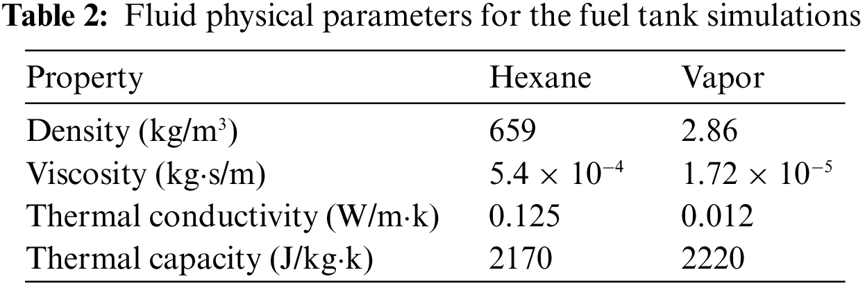
The simplified refuel pipe model and the simplified fuel tank model are depicted in Fig. 1. In this study, the diameter of the fueling pipe is set at 25.4 mm, and the diameter of the nozzle is set at 15 mm. Fig. 1a shows the transparent refueling pipe consisting of a 3D printed refueling tube and an extended horizontal tube. The regulating valve at the outlet is used to adjust the outflow pressure, which is used to equivalently represent different tank pressures. The vertical pipe is used to feed back the pressure at the outlet of the horizontal pipe. For safety concerns, only water is considered in our experiments, and the water is dyed to improve the visibility of fluid flow patterns in the pipe. Due to the limitation of the urea filling machine, two flow conditions, 14.6 and 17.1 L/min, are used in the experiment. For experimental precise positioning, two refueling positions (lower or upper location filling) are considered and represent two different directions of liquid inflow velocity. As for the corresponding simulation, we consider that the liquid phase is water for comparing the results with the experiment. The density of water and air are 998.2 and 1.225 kg/m3, respectively. The viscosity of water and air are 1.003 × 10−3 and 1.7984 × 10−5 kg⋅s/m, respectively.

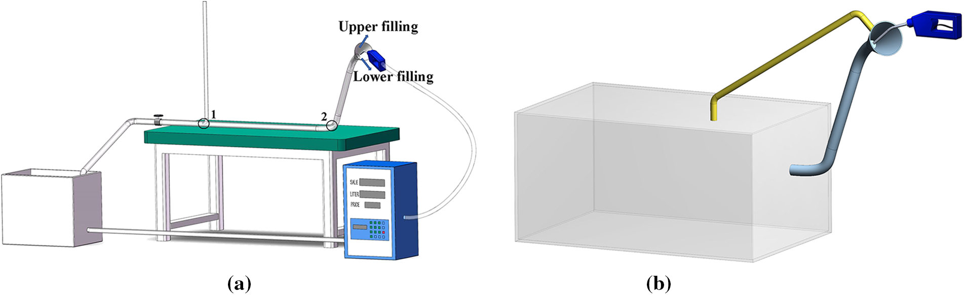
Figure 1: (a) Refueling pipe experimental set-up diagram and (b) the fuel tank simulation model

The simplified geometric model of the fuel filling system is shown in Fig. 1b. The fuel filling system simulation model included components such as a fuel pipe, a fuel tank, and a vapor return line. We employed the same fueling pipe and deleted the horizontal pipe in Fig. 1a. To simplify the calculation, the tank is simplified to a cuboid with the same volume as the real tank. The length, width, and height are 600 mm × 400 mm × 300 mm, and the vapor return line is a round pipe with a diameter of 15 mm. Only simulation was employed in the fuel tank refueling part. The liquid phase was changed to gasoline (hexane), and the other phases were air and gasoline vapor. Three different refueling flow rates (50, 60, and 70 L/min) were discussed in our simulations.

The boundary conditions in our simulations were velocity inlet and pressure outlet. The RNG k-ε turbulence model was employed for the unsteady and non-pressurizable flow during the refueling process. The hexane evaporation is considered in the tank refueling simulations. For meshing the pipes and tank, the tetrahedral grid was characterized by its flexibility and applicability to complex geometries. It greatly improved calculation efficiency while ensuring calculation accuracy and had unique advantages in simulating multi-phase flow. Therefore, we employed the ANSYS MESHING software to divide the mesh into tetrahedral meshes. Fig. 2 displayed the mesh size dependency on the overall static pressure and the mass-weighted average velocity for the simplified refuel pipe simulations. This study compared the overall static pressure and mass-weighted average velocity in the pipe over time, and the results were shown in Figs. 2a and 2b. When the number of grids increased from 670,000 to 1 million, the values of velocity and static pressure over time were almost the same, indicating that the number of grids did not significantly affect the calculation results and that a mesh with 670,000 cells was sufficient to simulate gas-liquid two-phase flow initiation and development behaviors with reasonable accuracy.

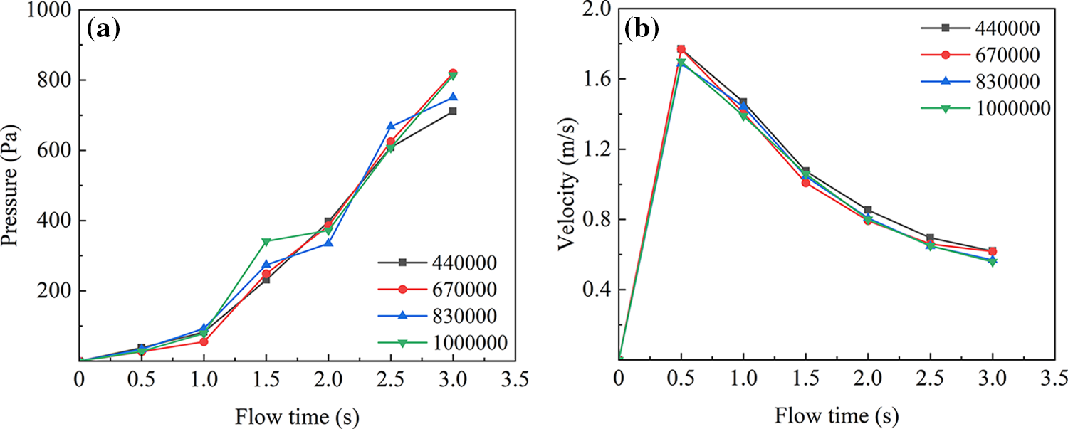
Figure 2: The change of static pressure and velocity with time in the pipe under different grid numbers: (a) the change of velocity with time, and (b) the change of static pressure with time

3  Results and Discussion

The transient flow behavior in fuel pipe refilling and simplified tank refueling were discussed respectively. We focused on the influence of different filling forms on the pipeline flow pattern in the former part and on the influence of gasoline evaporation on the filling of the tank in the latter.

3.1 Analysis of Fuel Pipe Refilling Results

3.1.1 Effect of Refueling Nozzle Position

We selected two different positions for the gasoline nozzle assembly, as shown in Fig. 1a, to study the backflow of liquid in the refueling pipe. In short, we called them upper filling mode and lower filling mode. Simulations and experimental studies were conducted to investigate different flow rate conditions. Firstly, we compared experimental and CFD simulated horizontal outlet flow pressures and liquid filling lengths in the inclined pipe, as shown in Table 1. The maximum error between the experimental and simulation comparison was controlled within 4%, indicating that the model used was highly reliable. The length of the inclined pipe was 39 cm, and we could easily observe that at a small flow rate of 14.6 L/min, the flow did not cause backflow, while the flow occurred backflow at 17.1 L/min when the gasoline nozzle was filled from the upper location. As shown in Table 1, when the refueling pipe is filled with a large flow rate (17.1 L/min), the reading in the lower filling mode is 30% higher than that of the inclined pipe filled in the upper filling mode, showing a stronger degree of counterflow. For lower location filling in large flow conditions, we compared experimental results with the simulation ones. Fig. 3 shows the backflow phenomenon, and we can see that there existed a large bubble at the second elbow in both the experiment and CFD simulation. The large bubble changes the flow pattern into slug flow, which is unfavorable for liquid flow inside the pipe [19,21].

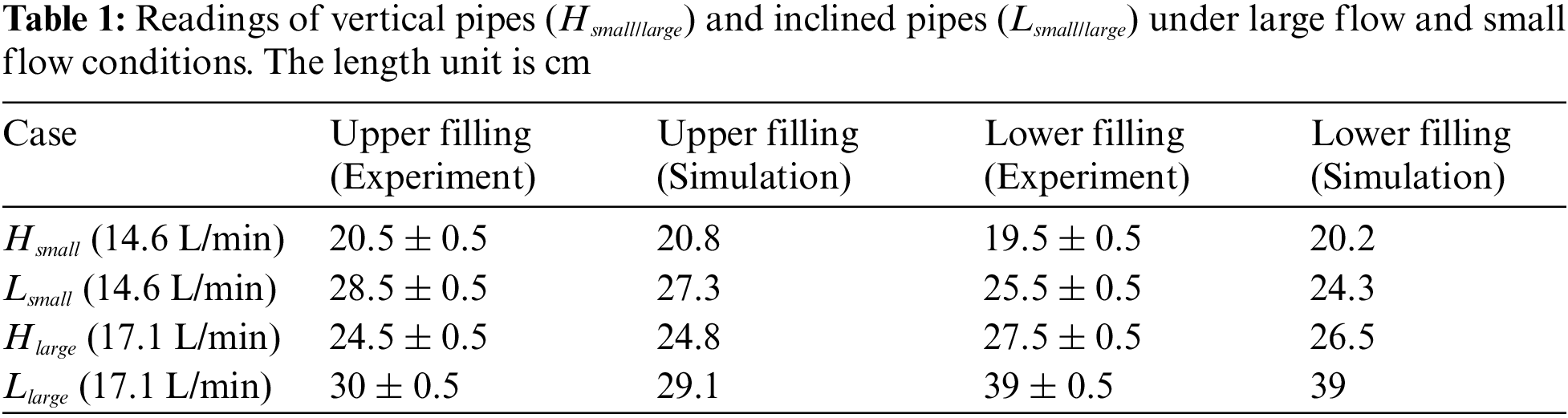
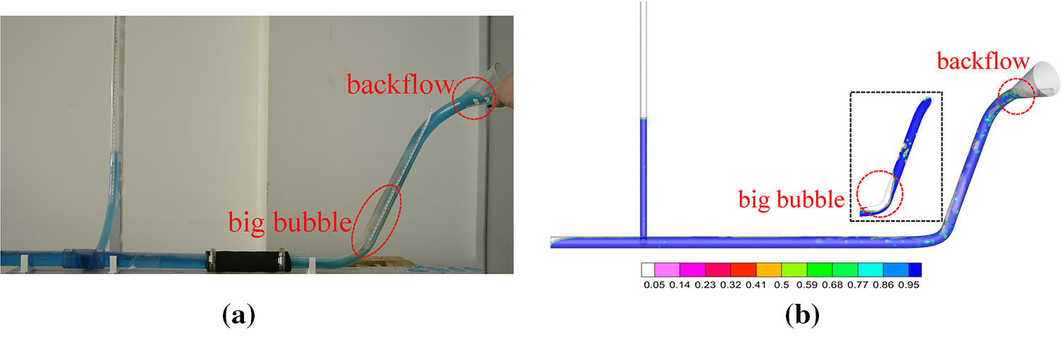
Figure 3: Comparison between the (a) experiment and (b) simulation of the fueling pipe under large flow condition

Table 1 and Fig. 3 demonstrated that our simulations were relatively accurate to explain the relevant mechanisms. Then, we focused on the pressure in the simulation. Two pressure monitoring points were set up inside the simplified refueling pipe, as shown in Fig. 1a. Monitoring points 1 and 2, located at the connection between the vertical and horizontal pipes and the second elbow, monitored the outflow pressure and elbow pressure at 17.1 L/min, as shown in Figs. 4a and 4b. The outflow pressure in Fig. 4a remained zero until water arrived at the valve and then rose sharply in a short time due to the water hammer effect. Then water filled the horizontal pipe, and the outflow rose slowly until the water filled the entire horizontal pipe at about 3.5 s. During that process, the second elbow at monitoring point 2 was not sealed by water, and the relative pressure remained nearly zero. Then the liquid seal was formed in the pipe, and water began to fill the incline pipe, which resulted in a sharp rise in both outflow and elbow pressure. After about 6 s, the pipe flow reached a steady state, and the relative pressure tended to be stable but fluctuated. We monitored the overall static pressure in the refueling pipe and presented the pressure evolution in Fig. 4c. The overall static pressure in the pipe increased before 5 s and then stabilized with fluctuations. The pressure patterns in Figs. 4a–4c were similar in the later refueling stage. We employed the fast Fourier transform (FFT) analysis to identify the frequency of the pressure from 10 to 20 s, and the results are shown in Figs. 4d–4f. The pressure fluctuations for the lower location refueling mode showed the characteristics of low-frequency and high-amplitude. In the upper filling mode, the pressure fluctuation was much weaker, and the pressure fluctuations showed high-frequency and low- amplitude characteristics, which avoided the backflow of liquid in the refueling pipe during high-flow condition refueling to a certain extent. Such pressure fluctuation patterns might be closely related to the flow patterns [6]. The slug flow in the lower filling model in Fig. 3 resulted in low-frequency and high-amplitude pressure characteristics, which are consistent with the results of the pressure fluctuation characteristics of the slug flow obtained in the experiments by Gourma et al. [14] and Fang et al. [15].

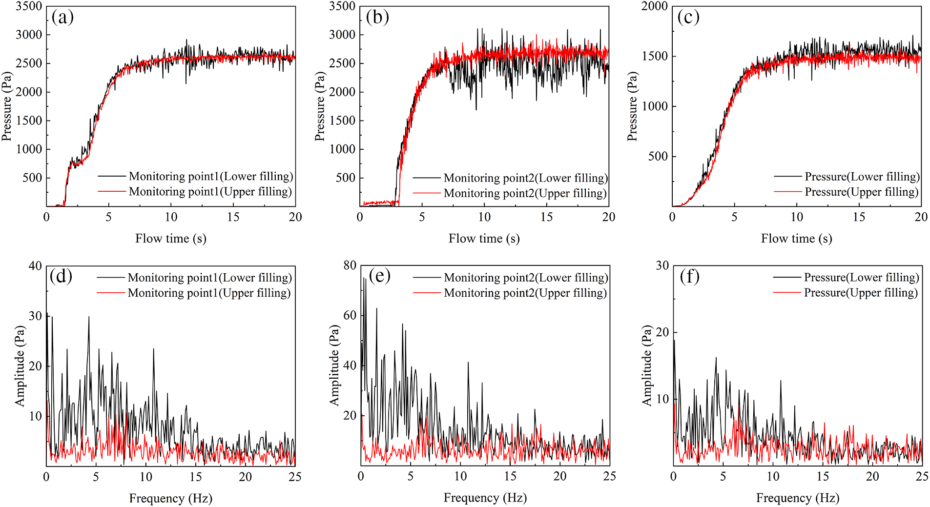
Figure 4: Pressure change curves of the fueling pipe at 17.1 L/min: (a) the outflow pressure at monitoring point 1, (b) the second elbow pressure at monitoring point 2, (c) static pressure of the whole pipe, (d) the outflow frequency spectrogram of pressure at monitoring point 1, (e) the second elbow frequency spectrogram of pressure at monitoring point 2, and (f) the whole pipe frequency spectrogram of static pressure

3.1.2 Gas-Liquid Flow Patterns

To investigate the specific reasons for the pressure fluctuation patterns in the pipe, we analyzed the flow pattern of the refueling pipe. Fig. 5 shows the water volume fraction contour at the pipe section 7 cross-sections of the inclined pipe at 10 and 20 s in all simulations and the flow pattern could be easily visualized. The oil filler and the inclined pipe were not in the same plane, so the fuel filler cross sections were not shown in Fig. 5. When refueling, bubbles of different shapes and sizes were continuously dispersed in the liquid phase in the inclined pipe due to air-water mixing, indicating a bubble-like flow pattern. The difference between the upper and low filling modes was the inflow flow direction. The flow would directly flush into the incline pipe in upper filling mode and hit the first elbow pipe in lower filling mode. The impact caused the water to quickly rebound and impact the lower pipe wall, resulting in the intensification of gas-liquid mixing. When the nozzle is located at a lower location, the strong mixing flow promotes the accumulation of tiny bubbles, eventually forming a large gas bubble. We could see there exist large bubbles at 20 s in lower filling mode, both at 14.6 and 17.1 L/min, while there were no large bubbles in upper filling mode. The elbow pipe between the horizontal and inclined pipe is the critical section for slug initiation due to liquid accumulation, which is consistent with the findings of Yin et al. [18]. At 17.1 L/min, the diameter of the large bubbles was close to the diameter of the pipe, occupying the entire overflow section, and blocking the liquid flow channel, impeding the flow of fluid inside the pipe, resulting in the phenomenon of alternating gas and liquid inside the pipe. During the experiment, an apparent liquid plug formed at the end of the beveled pipe of the refueling pipe, leading to an evident backflow phenomenon when the lower end of the refueling pipe was filled under a flow rate of 17.1 L/min. The tiny bubbles accumulated to form a large gas bubble, and fine bubbles were interspersed between the two gas bubbles. The flow pattern gradually evolved into slug flow pattern, which was unfavorable for the liquid flowing inside the pipe. These flow phenomena are consistent with the experimental results obtained by Alves et al. [21] and Rodrigues et al. [19].

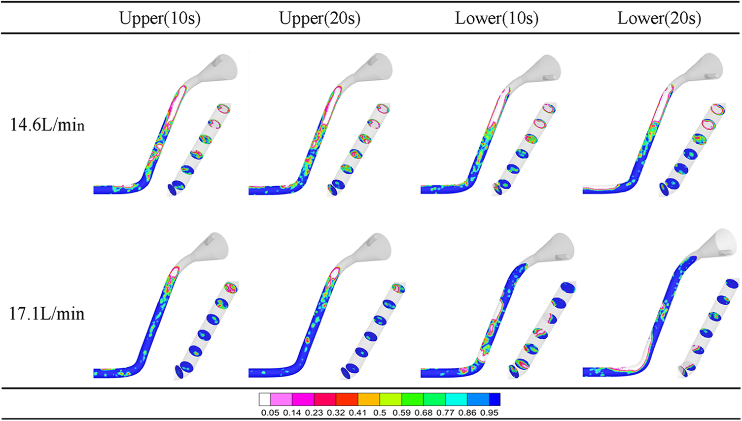
Figure 5: Contour of the water volume fraction at 10 and 20 s at the pipe section and cross-sections of refueling pipe for all cases

Fig. 6a shows the volume fraction of water inside the refueling pipe under different flow conditions at the upper and lower ends. The volume fraction of water inside the refueling pipe increased as the filling rate increased, which was due to the increase in liquid flow rate and the average liquid holdup in the pipe. Under high flow filling, the average liquid holdup of the upper filling was better than that of the lower filling because the slug flow pattern was generated during the lower filling. The alternations of large bubbles at the elbow were not conducive to the formation of a better liquid seal inside the pipe. Fig. 6b shows the average flow velocity in the entire pipe. Under the same refueling flow rate, the velocity in the lower filling mode was obviously smaller than that in the upper filling mode, indicating that higher intensity gas-liquid entrainment behavior would increase the resistance of the pipeline. Strong eddy-currents could occur in the bend pipe in fuel refueling pipes due to the impact of the liquid and the wall. Fuel crashes on the elbow pipe near the nozzle should be avoided to prevent high intensity gas-liquid entrainment behavior.

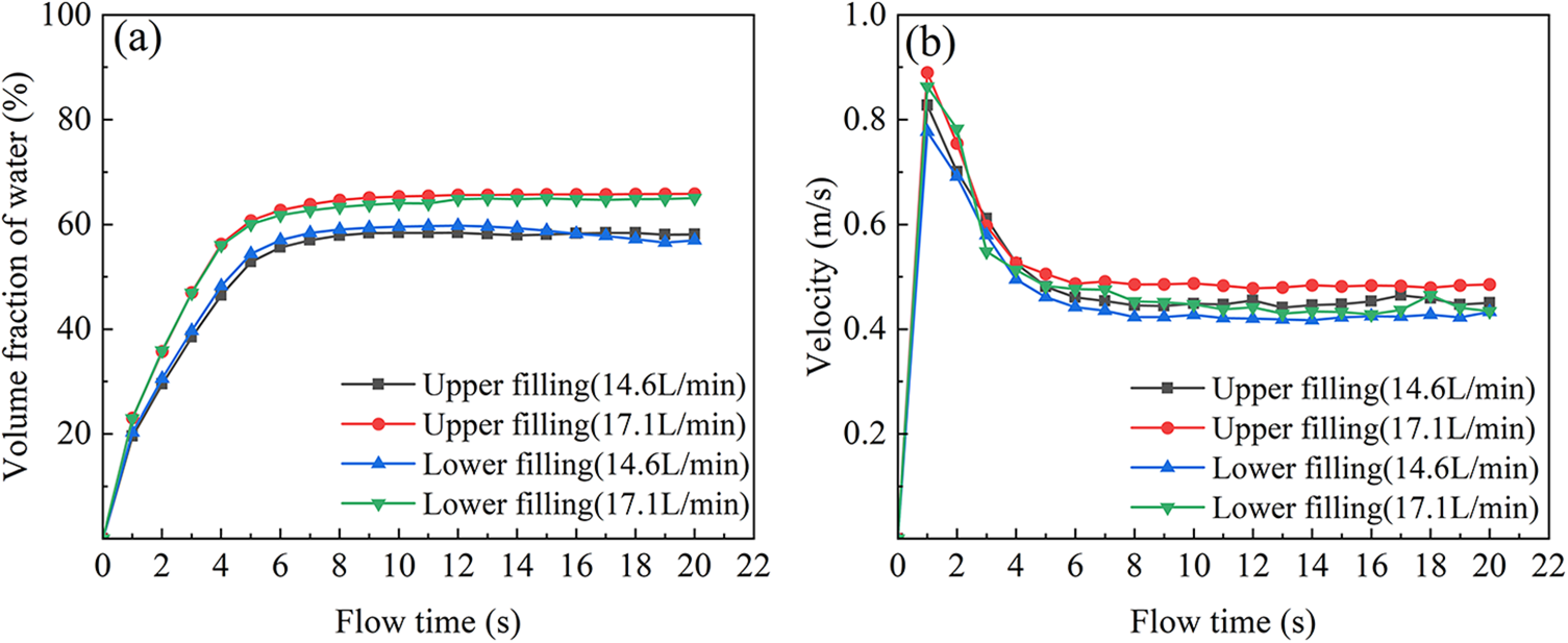
Figure 6: Comparison of the volume fraction and velocity of water when the filling pipe is filled with different filling rates at the upper and lower ends: (a) comparison of volume fraction of water over time, (b) comparison of velocity over time

3.2 Analysis of Tank Filling Results

During the refueling process in real life, gasoline evaporation is inevitable, which is a complex physicochemical process influenced by various factors. During refueling the tank, the fuel level rise rate varies with different refueling rates, making the refueling rate a crucial factor affecting gasoline evaporation. This section presented a simulation of the fuel refueling process using a simple refueling system to investigate the effects of refueling rate and fuel tank structure on gasoline evaporation. We considered the gasoline (hexane) evaporation process using the evaporative phase change model in Eq. (12) proposed by Lee [37] for the evaporative phase change. The wall temperature of the fuel tank is set at 310 K. According to the prompt in Section 3.1, we let gasoline flow directly flow into the inclined pipe and avoid hitting the first elbow. The relevant parameters of hexane and vapor are shown in Table 2. According to the previous investigation, the fuel refueling rate of most gas stations is between 50 and 70 L/min. The paper employed three different refueling flow rates: 50, 60, and 70 L/min.

3.2.1 Phase Change Mass Transfer Model Verification

To verify the accuracy of the phase change heat and mass transfer model in our UDF code, we adopted the initial conditions based on the analytical solution of Stephan’s problem [42] and conducted numerical simulations using the classical structure of the Stefan tube [33,43,44]. As depicted in Fig. 7a, the Stefan tube had dimensions of 15 cm height and 2 cm width, with the liquid hexane region at the bottom and the outlet boundary condition at the top. During the continuous diffusion of hexane from the bottom to the top of the tube by evaporation, the liquid level was kept constant while solving the heat and mass transfer equation. Fig. 7b compared the CFD simulated values of hexane vapor mass fraction with height against the analytical solution. The results indicated that the CFD predictions of the hexane mass fraction at different moments and heights were in excellent agreement with the analytical solution, thus demonstrating the reliability of the phase change heat and mass transfer model. By examining these factors, we aimed to gain insights into the gasoline evaporation process and inform strategies for minimizing fuel loss during refueling.

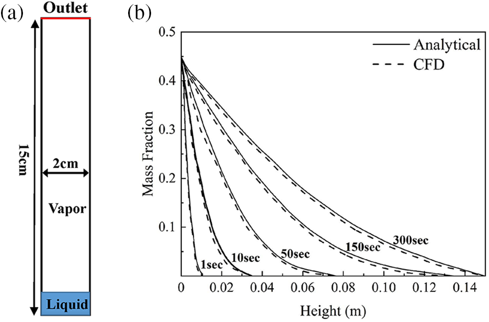
Figure 7: Verification of Stefan tube: (a) geometric model of Stefan tube, (b) comparison between the analytical solution of vapor hexane mass fraction varying with height and CFD simulation

3.2.2 Effect of Refueling Rate on Tank Filling

The hexane volume fraction during the fuel refueling process at different refueling rates was shown in Fig. 8. The average hexane vapor volume fraction in the tank was smaller than 5% was neglected and colored white. The hexane volatilization occurred on the liquid-solid interface. At the beginning of the refueling process, we could easily observe that a relatively high concentration of hexane vapor appeared at the bottom of the tank, around the parabolic fuel column and around the impact point between fuel and tank. The primary reason is that the fuel exhibits parabolic motion upon entering the tank, influenced by gravity, causing it to spread out on the bottom of the tank and splash around due to the impact on the tank wall. The splash phenomenon became more pronounced at higher refueling rates, which we could observe a larger hexane vapor area. After 20 s of filling, the fuel flow inside the tank became gentler compared to the previous flow state due to the fuel impact directly on the fuel surface instead of the tank wall at 50 and 60 L/min. Although there were still some liquid levels, violent splashing droplets were significantly reduced. However, at a refueling rate of 70 L/min, the fuel would directly hit the tank wall and splash, causing a high gasoline evaporation area. At the end of the refueling process (40 and 50 s), the fuel tank contained a certain amount of fuel, and the fuel tank inlet formed a liquid seal, which made it difficult for the fuel to splash out droplets. These fuel filling processes are consistent with the simulation results by Hassanvand et al. [31] and Hou et al. [33].

Figure 8: The hexane volume fraction at different refueling rates at different times

Fig. 9 displayed the mass average of vapor hexane at different refueling rates. The relative homogeneity and stability of the hexane molecules during the evaporation process results in a smaller average value and less variation in the mass of vapor hexane. The process of gasoline evaporation could be roughly divided into two stages:

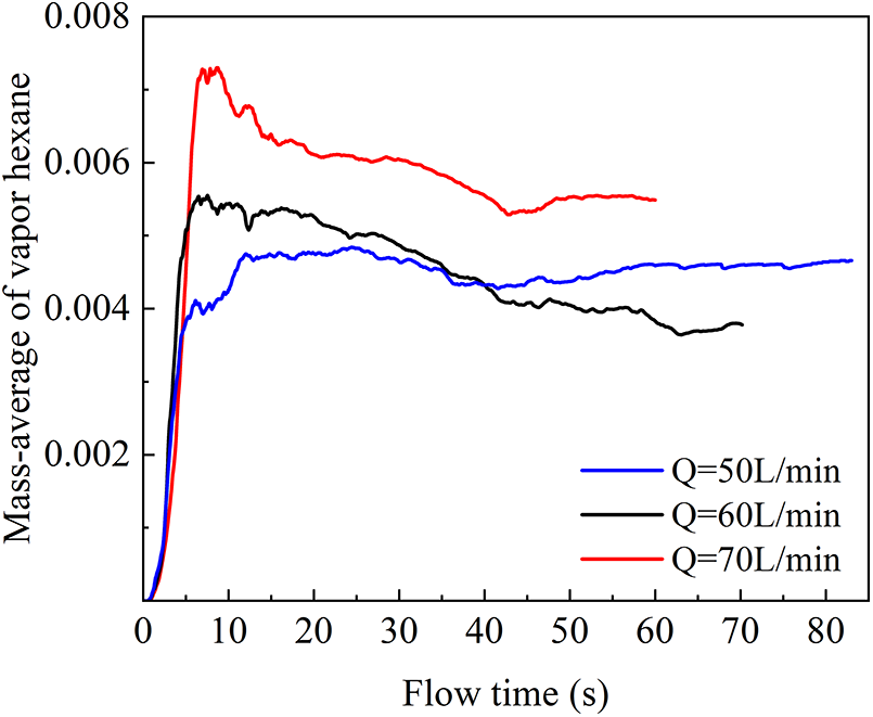
Figure 9: Mass-average of vapor hexane at different refueling rates

1. The early refueling period: the vaporized hexane content significantly increased during the initial refueling stage [35]. The average mass of vaporized hexane within the tank increased as the refueling rate increased [31]. When the refueling flow rate was higher, a faster refueling speed resulted in a more pronounced splashing phenomenon, which enhanced the convective heat transfer between the fuel and the air, leading to a substantial increase in the mass transfer area.

2. The smooth refueling period: the vapor content remained relatively stable. As the fuel level rose, the splash phenomenon of fuel droplets was moderated, and the fuel flow tended to calm down. The hexane volatilization occurred on the fuel surface. Consequently, the vapor content inside the tank slightly decreased during the later stages of refueling. When filling at a rate of 50 L/min, fuel flow inside the tank was smooth, and the vapor content was stable.

Fig. 10 shows the pressure evolutions in the tank and vapor return line in the early and middle stages at different filling flow rates. In high flow rate case (70 L/min), there was significant pressure fluctuation inside the tank, characterized by high-amplitude fluctuations, consistent with the tank pressure fluctuation measured by Dake et al. [1]. Such large pressure fluctuations at the refueling port of the tank would enhance the likelihood of backflow, which was unfavorable to the fuel filling process. After 25 s, the pressure fluctuation diminished. The possible reason was that the fuel entering the fuel tank directly contacts the liquid surface, and there was minimal splashing of droplets. In 50 and 60 L/min flow rate cases, the pressure fluctuation inside the tank was minor, and the filling process was relatively smooth. When refueling the fuel tank at a rate of 70 L/min, the pressure peak within the tank exhibited an increase of 800 Pa compared to the pressure peak recorded during refueling at the other two rates. Similarly, the pressure peak within the vapor return line was elevated by 400 Pa. These exceptionally high pressure peaks pose a significant detriment to the overall refueling process. In Fig. 10b, it could be seen that the pressure would have significant fluctuation in the 70 L/min flow rate filling. When decreasing the flow rate, the pressure fluctuations in the vapor return line became smaller. Actually, a higher flow rate would fill the tank faster but would also result in more volatilization of fuel and greater pressure fluctuations in the tank. The qualitative pressure fluctuation rules in storage tanks and vapor return lines were similar. Considering the filling efficiency and pressure fluctuations, the filling flow rate could be controlled at 60 L/min for the simplified tank.

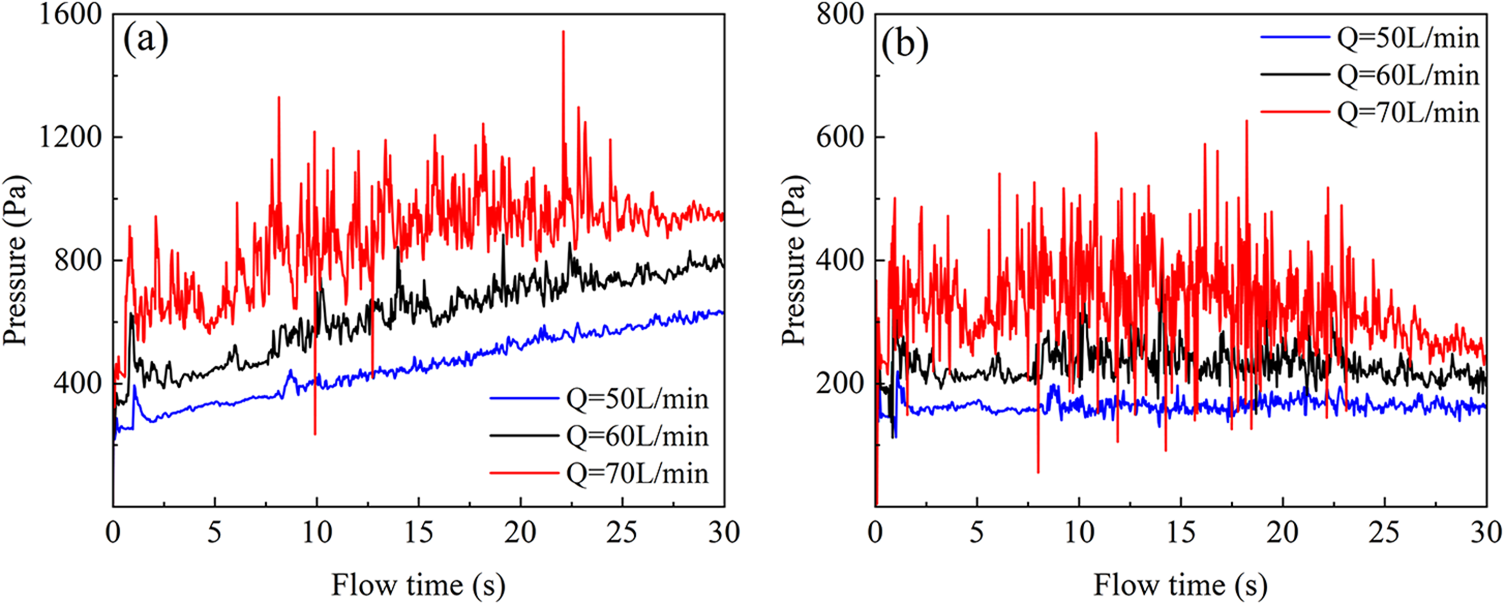
Figure 10: Pressure evolution at different refueling flow rates in the (a) fuel tank and (b) vapor return line

3.2.3 Effect of Fuel Tank Structure on Tank Filling

The flow pattern of fuel inside a tank is significantly impacted by the tank’s structure. Due to the varying shapes of tank structures, several factors related to these structures can influence the fuel flow, such as the tank refueling port location and slotting treatment. Thus, we explore these two factors. One is that we lower the height of the fuel filler to 100 mm from the bottom, and the other is that we introduce a slotting treatment at the bottom of the tank. Here, only 60 L/min flow rate is selected.

Fig. 11 displays the gasoline volume fraction nephogram of different fuel tank structures at various times. During the early stages of refueling (5 s), a lower tank refueling port weakened the impact of fuel when refueling to the bottom of the fuel, thereby reducing gasoline evaporation inside the tank. Then, after 20 s, the liquid seal reduced fuel evaporation. For the slotted tank, the raised bottom increased the mass transfer area at 5 s, resulting in more gasoline evaporation. At 10 s, half of the slotted bottom was filled with hexane, and the hexane vapor concentration area near the gasoline surface was large due to the impact between fuel and tank wall. It was essential to note that the flow pattern of fuel in the tank significantly impacted the evaporative emission of fuel, which increased with turbulence and the splash phenomenon generated by the flow. When the refueling time was 40 and 50 s, the fuel entered the late stage, the fuel level rose above the refueling port, and the flow became stable. During the late stage, the gasoline volume fraction nephogram for the slotted tank was similar to the initial tank.

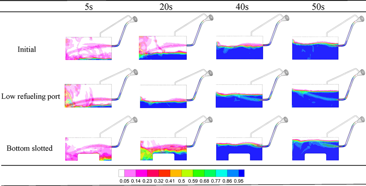
Figure 11: Hexane volume fraction nephogram of different fuel tank structures at different times

Fig. 12 presents the mass average of vapor hexane for different tank structures. The results indicated that the vapor hexane content sharply increases at the beginning of refueling for all three structures. The tank structure with a lower refueling port exhibited a significant decrease in vapor hexane inside the tank compared to the other two structures when the liquid seal was earlier formed, owing to the relatively smooth refueling process. However, the vapor hexane content in the tank with the slotted bottom remained high after a sharp rise.

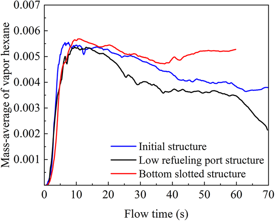
Figure 12: Mass-average of vapor hexane in different fuel tank structures

Fig. 13 shows the pressure evolution in fuel tank and vapor return line for the different fuel tank structures. In Fig. 13a, the internal pressure of the tank was shown for different structures. The internal pressure of all three structures showed a slow growth trend, with the lowered tank filling port structure displaying minor relative pressure fluctuation, and there will be no obvious pressure peak, which was lower than the pressure of the other two structures after stabilization. The initial structural pressure experienced multiple high-amplitude fluctuations, with the highest pressure peak approaching 900 Pa. For both changed tank structures, the pressure fluctuations were small. Fig. 13b illustrates the pressure of the vapor return line for different tank structures. The tank structure with a lower refueling port exhibited a decreasing trend in the middle and later stages of refueling, which had a significant impact on gasoline evaporation. In the tank’s structural design, a lower refueling port of the tank could decrease the tank pressure and the slotted design would increase the transfer area, increasing the tank pressure but lowering the tank pressure fluctuations.

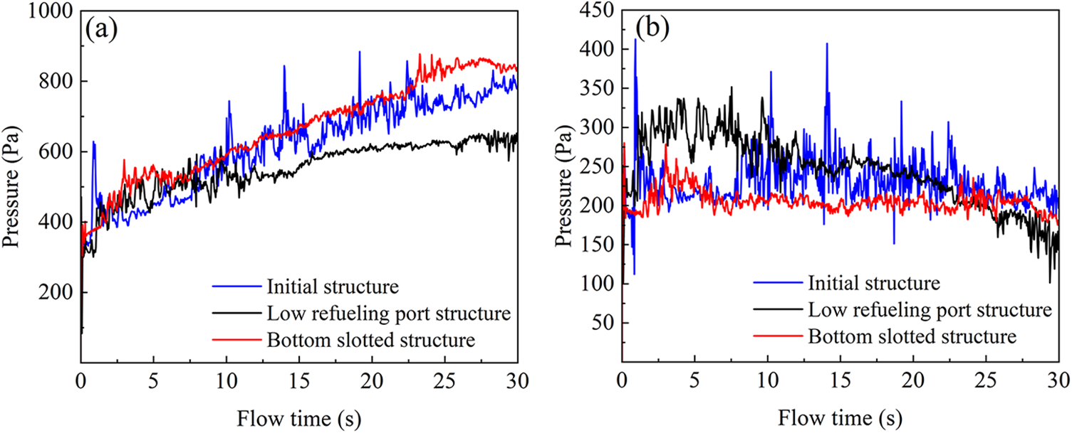
Figure 13: Pressure evolution for the different fuel tank structures in the (a) fuel tank and (b) vapor return line

4  Conclusion

The pressure fluctuation plays a crucial role in the oil refueling system. By monitoring pressure fluctuations, the effects of the nozzle flow rate and direction on the refueling pipe and the effects of the flow rate and tank structures on the entire tank have been discussed. The following conclusions can be drawn:

(1) The experimental and simulation results indicate that the likelihood of backflow in the refueling pipe rises with the refueling rate. Direct liquid flow into the inclined pipe results in a bubbly flow formation inside the refueling pipe. In the bubbly flow, the gas phase is distributed in the form of dispersed bubbles that continuously generate and collapse and have minimal influence on the pressure difference fluctuation. Besides, the stable liquid seal is formed inside the fuel pipe, which enhances filling smoothness.

(2) When the liquid flushes to the elbow near the inlet, it will intensify the gas-liquid mixing. The pressure at the end of the refueling pipe in the lower located nozzle case is 30% higher than that in the upper located nozzle case at a high flow rate. Due to the high-speed flow of the fuel and the curvature of the pipeline, intense vortices and turbulence will form, leading to an increased degree of gas-liquid mixing, which causes a change of flow pattern in the inclined pipe from bubbly flow to slug flow. The FFT analysis shows that the pressure fluctuation of the slug flow is more severe than that of the bubble flow, and the differential pressure fluctuation exhibits low frequency and high amplitude, which results in a backflow phenomenon. Thus, the slug flow during the refueling process should be avoided.

(3) Both filling efficiency and pressure fluctuations should be concerned in the fueling process. For the entire tank refueling, hexane evaporation is considered. As the filling rate increases, it is an indication of higher filling efficiency. When refueling the fuel tank at a rate of 70 L/min, the pressure peak within the tank exhibited an increase of 800 Pa compared to the pressure peak recorded during refueling at the other two rates. Nevertheless, this can lead to an intensified splashing phenomenon at the beginning of fueling, causing a significant increase not only in the hexane content of the fuel vapor but also in the tank pressure fluctuations. Injected fuel directly contacting the liquid surface or forming liquid seal for the refueling port can decrease the pressure fluctuations. It is essential to choose a moderate filling flow rate for the gasoline refueling with reasonable pressure fluctuations and take into account the balance of the filling efficiency and safety.

(4) The study analyzes the structural parameters of the fuel tank, including the location of the refueling port and slotting treatment. The results show that the vapor hexane content inside the tank increases sharply in all three structures due to fuel splashing. However, for the tank structure with a lower refueling port, the occurrence of a liquid seal in the early stages of refueling leads to the evaporation rates of vapor hexane lower than 0.004 kg/s during the middle and final stages. In contrast, the tank structure with a slotted bottom exhibits high vapor hexane content throughout the refueling process, likely due to the increased impact area of the fuel in the tank wall. Nevertheless, the peak pressure of the fuel tank and vapor return line is reduced by about 200 Pa relative to the initial tank structure, which is favorable for refueling safety.

Acknowledgement: Not applicable.

Funding Statement: This work was supported by the National Natural Science Foundation of China with Grant No. 12002334 for C.Z., Zhejiang Provincial Natural Science Foundation (Grant No. LQ21A020004 for C.Z.) and the Excellent Youth Natural Science Foundation of Zhejiang Province, National Science Foundation of Anhui Province (2108085QE226), China (No. LR21E060001 for L.Q. and C.Z.). C.Z. acknowledges the China Scholarship Council (No. 202108330166) for providing him with a visiting scholarship at NUS, Singapore.

Author Contributions: The authors confirm contribution to the paper as follows: study conception and design: Chenlin Zhu,Yan Zhao; data collection: Yan Zhao, Lifang Zeng; analysis and interpretation of results: Yan Zhao, Chenlin Zhu, Lifang Zeng, Lijuan Qian; draft manuscript preparation: Yan Zhao, Zhitao Jiang, Jiafeng Xie. All authors reviewed the results and approved the final version of the manuscript.

Availability of Data and Materials: All data generated or analysed during this study are included in this published article.

Conflicts of Interest: The authors declare that they have no conflicts of interest to report regarding the present study.

References

1. Dake, M. (2018). Computer aided engineering of an automobile gasoline refueling system (Ph.D. Thesis). Colorado State University, USA. [Google Scholar]

2. Stoker, T. M. (2019). Experimental investigation of automotive refueling system flow and emissions dynamics to support CFD development (Ph.D. Thesis). Colorado State University, USA. [Google Scholar]

3. Banerjee, R., Isaac, K., Oliver, L., Breig, W. (2002). Features of automotive gas tank filler pipe two-phase flow: Experiments and computational fluid dynamics simulations. Journal of Engineering for Gas Turbines and Power, 124(2), 412–420. [Google Scholar]

4. Mastroianni, M., Savoni, L., Henshaw, P., Rankin, G. W. (2011). Experimental study of fuel tank filling. International Journal of Mechanical and Mechatronics Engineering, 5(10), 1998–2005. [Google Scholar]

5. Gunnesby, M. (2015). On flow predictions in fuel filler pipe design-physical testing vs computational fluid dynamics (Master Thesis). Department of Management and Engineering Division of Applied Thermodynamics and Fluid Mechanics, Linköpings University, Sweden. [Google Scholar]

6. Matsui, G. (1986). Automatic identification of flow regimes in vertical two-phase flow using differential pressure fluctuations. Nuclear Engineering and Design, 95, 221–231. [Google Scholar]

7. Cui, B., Chen, P., Zhao, Y. (2022). Numerical simulation of particle erosion in the vertical-upward-horizontal elbow under multi-phase bubble flow. Powder Technology, 404, 117437. [Google Scholar]

8. Yang, B., Jafarian, M., Freidoonimehr, N., Arjomandi, M. (2022). Trajectory of a spherical bubble rising in a fully developed laminar flow. International Journal of Multi-Phase Flow, 157, 104250. [Google Scholar]

9. Kole, M., Shah, R. K., Khandekar, S. (2022). Energy efficient thermal management at low reynolds number with air-ferrofluid taylor bubble flows. International Communications in Heat and Mass Transfer, 135, 106109. [Google Scholar]

10. Goncalves, G. F., Matar, O. K. (2022). Mechanistic modelling of two-phase slug flows with deposition. Chemical Engineering Science, 259, 117796. [Google Scholar]

11. Li, H., Hrnjak, P. (2023). A mechanistic model in annular flow in microchannel tube for predicting heat transfer coefficient and pressure gradient. International Journal of Heat and Mass Transfer, 203, 123805. [Google Scholar]

12. Jia, S., Dong, C. (2023). Flow and heat transfer model for turbulent-laminar/turbulent gas-liquid annular flows. Applied Thermal Engineering, 219, 119431. [Google Scholar]

13. Liu, W., Lv, X., Zhao, Z. (2020). Effect of swirl on fluctuation of pressure drop in a gas-liquid slug flow. Measurement: Sensors, 10, 00019. [Google Scholar]

14. Gourma, M., Verdin, P. G. (2016). Two-phase slug flows in helical pipes: Slug frequency alterations and helicity fluctuations. International Journal of Multi-Phase Flow, 86, 10–20. [Google Scholar]

15. Fang, L. P., Meng, L. Y., Liu, C. W., Li, Y. X. (2021). Experimental study on the amplitude characteristics and propagation velocity of dynamic pressure wave for the leakage of gas-liquid two-phase intermittent flow in pipelines. International Journal of Pressure Vessels and Piping, 193, 104457. [Google Scholar]

16. Danielson, T. J., Bansal, K. M., Djoric, B., Larrey, D., Johansen, S. T. et al. (2012). Simulation of slug flow in oil and gas pipelines using a new transient simulator. Offshore Technology Conference, OnePetro. [Google Scholar]

17. Badarudin, A., Setyawan, A., Dinaryanto, O., Widyatama, A. (2018). Interfacial behavior of the air-water counter-current two-phase flow in a 1/30 scale-down of pressurized water reactor (PWR) hot leg. Annals of Nuclear Energy, 116, 376–387. [Google Scholar]

18. Yin, P., Cao, X., Li, Y., Yang, W., Bian, J. (2018). Experimental and numerical investigation on slug initiation and initial development behavior in hilly-terrain pipeline at a low superficial liquid velocity. International Journal of Multi-Phase Flow, 101, 85–96. [Google Scholar]

19. Rodrigues, R. L., Bertoldi, D., dos Santos, E. N., Schneider, F. A., da Silva, M. J. et al. (2019). Experimental analysis of downward liquid-gas slug flow in slightly inclined pipes. Experimental Thermal and Fluid Science, 103, 222–233. [Google Scholar]

20. Rodrigues, R. L., Cozin, C., Naidek, B. P., Neto, M. A. M., da Silva, M. J. et al. (2020). Statistical features of the flow evolution in horizontal liquid-gas slug flow. Experimental Thermal and Fluid Science, 119, 110203. [Google Scholar]

21. Alves, R. F., Schneider, F. A., Barbuto, F. A., Santos, P. H., Morales, R. E. (2019). An experimental analysis on the influence of flow direction changes on the transitions in gas-liquid, slug-to-stratified downward flows. International Journal of Multi-Phase Flow, 119, 155–165. [Google Scholar]

22. Akhlaghi, M., Taherkhani, M., Nouri, N. M. (2020). Study of intermittent flow characteristics experimentally and numerically in a horizontal pipeline. Journal of Natural Gas Science and Engineering, 79, 103326. [Google Scholar]

23. Dhar, M., Ray, S., Das, G., Das, P. K. (2022). Hydraulic jump induced flooding and slugging in stratified gas-liquid flow—An experimental appraisal. Experimental Thermal and Fluid Science, 134, 110617. [Google Scholar]

24. Ma, Y., Zeng, S., Shao, J., Zhou, T., Lyu, J. et al. (2023). An experimental study on gas-liquid two-phase countercurrent flow limitations of vertical pipes. Experimental Thermal and Fluid Science, 141, 110789. [Google Scholar]

25. Thaker, J., Banerjee, J. (2017). Transition of plug to slug flow and associated fluid dynamics. International Journal of Multi-Phase Flow, 91, 63–75. [Google Scholar]

26. Rahmandhika, A., Widyatama, A., Dinaryanto, O., Widyaparaga, A., Indarto, et al. (2019). Experimental study on the hydrodynamic behavior of gas-liquid air-water two-phase flow near the transition to slug flow in horizontal pipes. International Journal of Heat and Mass Transfer, 130, 187–203. [Google Scholar]

27. Mohmmed, A. O., Al-Kayiem, H. H., Osman, A., Sabir, O. (2020). One-way coupled fluid-structure interaction of gas-liquid slug flow in a horizontal pipe: Experiments and simulations. Journal of Fluids and Structures, 97, 103083. [Google Scholar]

28. Cao, X., Zhang, P., Li, X., Li, Z., Zhang, Q. et al. (2022). Experimental and numerical study on the flow characteristics of slug flow in a horizontal elbow. Journal of Pipeline Science and Engineering, 2(4), 100076. [Google Scholar]

29. Mackay, D., Matsugu, R. S. (1973). Evaporation rates of liquid hydrocarbon spills on land and water. The Canadian Journal of Chemical Engineering, 51(4), 434–439. [Google Scholar]

30. Stiver, W., Mackay, D. (1984). Evaporation rate of spills of hydrocarbons and petroleum mixtures. Environmental Science & Technology, 18(11), 834–840. [Google Scholar]

31. Hassanvand, A., Hashemabadi, S., Bayat, M. (2010). Evaluation of gasoline evaporation during the tank splash loading by CFD techniques. International Communications in Heat and Mass Transfer, 37(7), 907–913. [Google Scholar]

32. Xu, Z., Zhang, Y., Li, B., Huang, J. (2016). Modeling the phase change process for a two-phase closed thermosyphon by considering transient mass transfer time relaxation parameter. International Journal of Heat and Mass Transfer, 101, 614–619. [Google Scholar]

33. Hou, Y., Chen, J., Zhu, L., Sun, D., Li, J. et al. (2017). Numerical simulation of gasoline evaporation in refueling process. Advances in Mechanical Engineering, 9(8), 1687814017714978. [Google Scholar]

34. Mohammed, H. I., Giddings, D., Walker, G. S. (2019). CFD multi-phase modelling of the acetone condensation and evaporation process in a horizontal circular tube. International Journal of Heat and Mass Transfer, 134, 1159–1170. [Google Scholar]

35. Romagnuolo, L., Frosina, E., Andreozzi, A., Senatore, A., Fortunato, F. (2021). Experimental analysis of evaporative emissions of ethanol-blended gasoline in automotive tanks at different temperature conditions. Fuel, 304, 121427. [Google Scholar]

36. Brackbill, J. U., Kothe, D. B., Zemach, C. (1992). A continuum method for modeling surface tension. Journal of Computational Physics, 100(2), 335–354. [Google Scholar]

37. Lee, W. (1980). A pressure iteration scheme for two-phase flow modeling. Washington DC, USA: Multi-Phase Transport Fundamentals, Reactor Safety, Applications, Hemisphere Publishing. [Google Scholar]

38. Rashid, M. T., Li, J., Chen, X., Song, A., Wang, N. (2021). Numerical simulation of evaporation phenomena and heat transfer of liquid hydrocarbon in a microtube. International Journal of Heat and Mass Transfer, 179, 121734. [Google Scholar]

39. Wang, Q., Li, M., Xu, W., Yao, L., Liu, X. et al. (2020). Review on liquid film flow and heat transfer characteristics outside horizontal tube falling film evaporator: CFD numerical simulation. International Journal of Heat and Mass Transfer, 163, 120440. [Google Scholar]

40. Abood, S., Abdulwahid, M., Almudhaffar, M. (2019). Comparison between the experimental and numerical study of (air-oil) flow patterns in vertical pipe. Case Studies in Thermal Engineering, 14, 100424. [Google Scholar]

41. Wang, Z., He, Y., Duan, Z., Huang, C., Yuan, Y. et al. (2022). Effects of rolling motion on transient flow behaviors of gas-liquid two-phase flow in horizontal pipes. Ocean Engineering, 255, 111482. [Google Scholar]

42. Abianeh, O. S., Chen, C. (2012). A discrete multicomponent fuel evaporation model with liquid turbulence effects. International Journal of Heat and Mass Transfer, 55(23–24), 6897–6907. [Google Scholar]

43. Sun, D. L., Xu, J. L., Wang, L. (2012). Development of a vapor-liquid phase change model for volume-of-fluid method in fluent. International Communications in Heat and Mass Transfer, 39(8), 101–1106. [Google Scholar]

44. Sun, D., Xu, J., Chen, Q. (2014). Modeling of the evaporation and condensation phase-change problems with fluent. Numerical Heat Transfer, Part B: Fundamentals, 66(4), 326–342. [Google Scholar]