
 Submit a Paper
 Propose a Special lssue
 Open Access
ARTICLE

A Numerical Study of the Double Diffusivity with Convective and Radiative Turbulent Flow in a Greenhouse with Humidity Sources
1 División de Estudios de Posgrado e Investigación, Tecnológico Nacional de México/IT de Pachuca, Carretera México-Pachuca km. 87.5, Colonia Venta Prieta, Pachuca de Soto, 42080, México
2 Laboratorio de Biología Celular y Molecular, Facultad de Ciencias Naturales, Campus Juriquilla, Universidad Autónoma de Querétaro, Av. de las Ciencias S/N, Juriquilla, Querétaro, 76320, México
3 División Académica de Ingeniería y Arquitectura, Universidad Juárez Autónoma de Tabasco, (DAIA-UJAT) Carretera Cunduacán-Jalpa de Méndez km. 1, Cunduacán, 86690, México
* Corresponding Author: K. M. Aguilar-Castro. Email:
(This article belongs to the Special Issue: Innovative Cooling Systems: Design, Optimization, and Applications)
Frontiers in Heat and Mass Transfer 2025, 23(6), 1741-1765. https://doi.org/10.32604/fhmt.2025.069560
Received 26 June 2025; Accepted 18 August 2025; Issue published 31 December 2025
 View Full Text
 Download PDF
Abstract
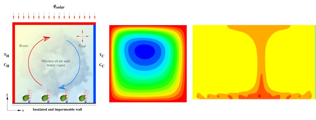
A numerical study analyzed double diffusion caused by convective and radiative heat transfer in a greenhouse with and without internal humidity sources. Two cases were examined: one considering temperature and mass concentration gradients on vertical walls and another incorporating internal humidity sources, enhancing convective and diffusive flows. Four configurations were analyzed by varying the length of the greenhouse, and the Rayleigh number was calculated over a range from 2.29 × 10¹⁰ to 6.07 × 10¹². Simulations modeled the greenhouse interior six times a day (8:00 a.m. to 7:00 p.m.), accounting for external temperature, humidity, and solar radiation. The Finite Volume Method solved the governing equations using the k-ε turbulence model for the turbulent flow regime. Results showed a maximum temperature of 50°C at 2:50 p.m. and a relative humidity of 84.12%. Adjusting inlet temperature and humidity effectively mitigated external weather effects. Adding humidity sources improved greenhouse performance, increasing humidity concentration by 4.93 to 5.35 times, particularly at 2:50 and 4:20 p.m. Convective and radiative Nusselt and Sherwood numbers were plotted for both cases, revealing higher humidity levels with internal sources, highlighting their importance in optimizing greenhouse microclimates.Graphic Abstract
Keywords
Nomenclature
| Concentration of humidity, | |
| Concentration of ambient humidity, | |
| Concentration of humidity at the mixture inlet, | |
| Concentration of humidity at the mixture outlet, | |
| Concentration of source of humidity, | |
| Specific heat (Air-H2O), | |
| Specific heat of the conductive wall, | |
| Constants of the | |
| Diffusion coefficient, | |
| View factor. | |
| Acceleration of gravity, | |
| Convective heat transfer coefficient outside, | |
| Cavity height, | |
| Lewis number, | |
| Local Nusselt number. | |
| Average Nusselt number. | |
| Fluid pressure, | |
| Prandtl number, | |
| Wall heat flux, | |
| Outside convective heat flux, | |
| Indoor convective heat flux, | |
| Outside radiative heat flux, | |
| Rayleigh number. | |
| Local Sherwood number. | |
| Average Sherwood number. | |
| Cavity width, | |
| Greek Symbols | |
| Thermal diffusivity, | |
| Volumetric expansion coefficient | |
| Emissivity | |
| Rate of Dissipation of | |
| Temperature distribution effectiveness | |
| Concentration distribution effectiveness | |
| Turbulence kinetic energy, | |
| Thermal conductivity (mixed), | |
| Dynamic viscosity (Air-H2O), | |
| Mixture density (Air-H2O), | |
| Reflectivity | |
| Stefan-Boltzmann constant, | |
| Transmissivity | |
Greenhouse agriculture is critical in ensuring food security, yet it faces increasing challenges due to climate change. Fluctuating temperature and humidity levels inside greenhouses can negatively impact crop growth and productivity, necessitating optimized environmental control strategies. This need has spurred extensive research into improving the thermal and hydric efficiency of greenhouses, with a particular focus on balancing energy use and crop yield.
One area of focus has been the relationship between greenhouse geometry and natural convection. For instance, Paing and Anderson [1] found that reducing the aspect ratio and roof pitch decreased convective heat transfer by 25% and 15%, respectively, offering insights into energy-efficient greenhouse design. Similarly, Yanru et al. [2] highlighted significant spatial temperature variations in plastic greenhouses, identifying soil temperature as a stable heat source. Together, these studies underscore the potential of design modifications to improve thermal efficiency.
Research has also examined the impact of climate control technologies. Nezir Yağız Çam et al. [3] demonstrated that optimized climate control mechanisms, such as heat pumps, could significantly reduce temperature deviations in greenhouses in diverse climatic regions like Türkiye and Qatar. While studies like those by Mao and Su (2024) [4] leverage CFD models to predict internal conditions accurately, Almashharawi et al. (2024) [5] introduce innovative liquid desiccant systems for climate control and water savings. Similarly, Mao and Li (2024) [6] provide insights into how wind conditions and crop height influence microclimate dynamics in multi-span greenhouses. These advancements highlight the need for integrated approaches considering external variables and cutting-edge technologies in greenhouse design.
Evaporative cooling has emerged as another effective method for temperature regulation. Mardomakdeh et al. [7] assessed its application in Tehran, highlighting its potential for water-efficient cooling during peak summer months. Similarly, Jiaming Guo et al. [8] evaluated roof sprinkler systems for reducing summer temperatures, demonstrating the viability of cost-effective cooling strategies. These findings collectively emphasize the critical role of water-based cooling systems in hot climates.
Thermal modeling has further expanded our understanding of heat transfer within greenhouses. Chol-Ho An et al. [9] demonstrated the feasibility of winter cultivation in solar double plastic-covered greenhouses, maintaining critical temperature thresholds. Meanwhile, Zhang et al. [10] explored multilayer wall designs for Chinese solar greenhouses, finding minimal coupling between heat and moisture transfer, an attribute that enhances thermal stability. These studies highlight the importance of structural innovations in greenhouse design.
Advanced automation and energy-efficient technologies are increasingly being integrated into greenhouses. Kavga et al. [11] explored automation through CFD modeling, while Saberian and Sajadiye [12] utilized CFD to address extreme summer temperatures in Ahvaz, Iran. Carlini et al. [13] extended this work by analyzing non-uniform temperature distributions to optimize designs further. Notably, Han et al. [14] investigated active-passive heat storage technologies, providing methods to reduce fossil energy dependency during off-seasons.
Despite these advancements, limitations remain. Many studies, such as those by Wang et al. [15] and Saud Ghani et al. [16], have focused on specific cooling or heating strategies without considering the interaction between convective and radiative heat transfer. Moreover, the influence of dynamic external climatic factors, such as solar radiation and ambient humidity, on greenhouse microclimates has not been extensively explored. Additionally, studies like Morteza Taki et al. [17] and Tong et al. [18] have emphasized localized conditions without generalizing findings to diverse climatic scenarios.
The bibliographic review reveals that various studies have explored the internal environment of greenhouses under different climatic conditions. However, despite these advancements, certain aspects remain underexplored. While many studies focus on temperature regulation, the specific interaction between convective and radiative heat transfer combined with double diffusion in greenhouses with internal humidity sources has received limited attention. The influence of time-dependent external climatic factors, such as solar radiation and ambient humidity, on greenhouse microclimates has not been extensively studied. This research addresses these gaps by shedding light on extreme climate conditions in a region of Mexico, focusing on specific characteristics and scenarios that have not been previously examined.
The objective of the present study is to conduct a numerical investigation of double diffusion driven by convective and radiative heat transfer in a greenhouse, both with and without internal sources of humidity. This work integrates findings from studies such as Yu et al. [19], Abid et al. [20], Xiao et al. [21], Jehhef et al. [22], Gomez-Zavaglia et al. [23], and Zeroual et al. [24], ensuring a comprehensive approach that bridges existing knowledge gaps. This work has incorporated a large number of parameters that have not been included in previous studies, which has greatly increased the complexity of the study model. The intention is to get as close as possible to the actual climatic conditions of greenhouse operation.
This research aims to provide insights into optimizing greenhouse environments for improved energy efficiency and crop productivity by analyzing the hydrothermal regime under various configurations and external conditions. The novelty of this study is the combination of convective and radiative fluxes over a wide range of Ra numbers. The results provide information on the behavior of temperature and humidity variables from 8 a.m. to 7 p.m. The information is of considerable interest for improving the performance of greenhouse crops.
The physical model represents a closed cavity where temperature and concentration gradients are imposed. This phenomenon, known as double diffusion, generates convective movement. In previous studies, Serrano-Arellano et al. [25,26] have presented the effects of assisted and opposite double diffusion, indicating that the direction of double diffusion affects fluid movement, either benefiting or hindering convective movement. In this study, assisted double diffusion was considered to favor convective movement.
The physical model is a simplification of the geometry of a greenhouse. The cavity changes geometry from square to rectangular for two case studies. Solar radiation falls on the upper surface, and a constant temperature and humidity concentration are imposed on the side walls.
It is worth mentioning that radiative exchange between the cavity walls was taken into account to quantify the convective and radiative Nusselt numbers.
The left and upper walls are affected by radiative heat flux, which varies throughout the day to simulate solar radiation. In the first case study (Fig. 1a), no humidity sources were considered inside; the double diffusion is caused solely by the temperature and mass gradients of the interior surfaces.
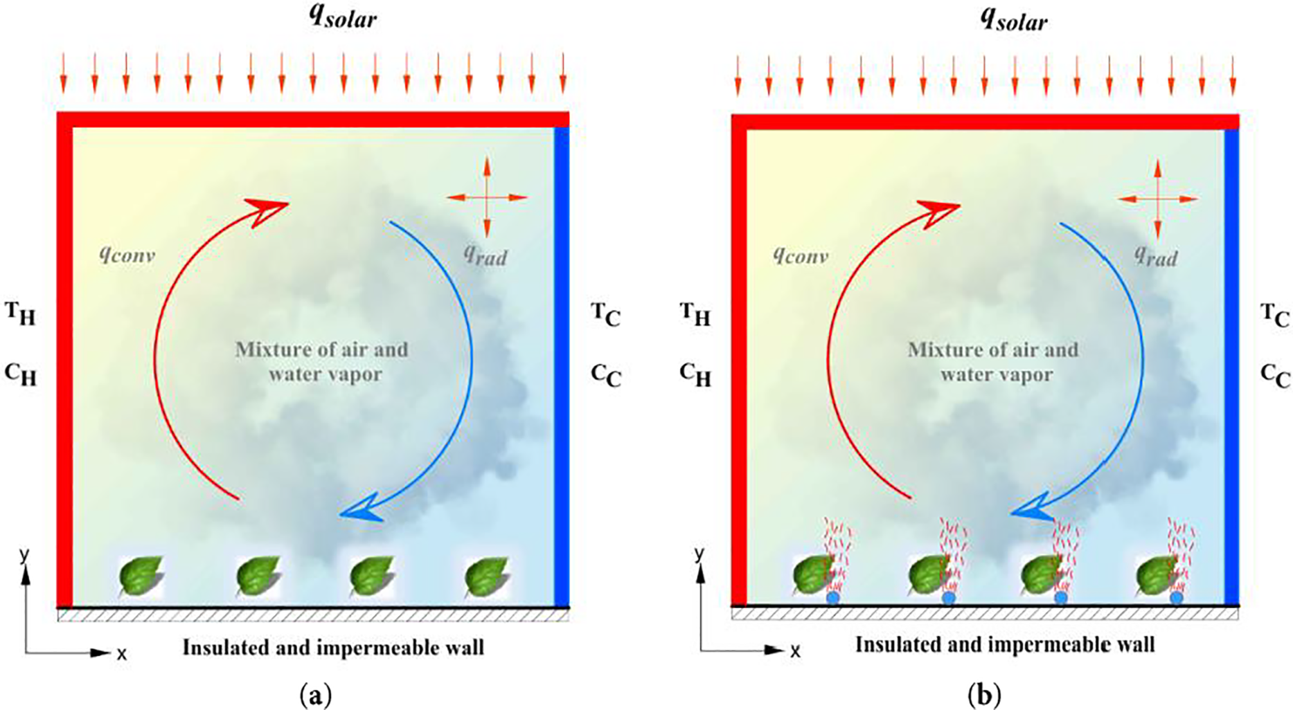
Figure 1: Physical model of the cavity; (a) without humidity sources (b) with humidity sources
The second case study is presented in Fig. 1b. In this case, in addition to considering diffusion gradients on the surfaces, humidity sources inside the greenhouse were considered. The number of humidity sources was varied from 10 to 100 in increments of 10 to analyze the mass diffusion effect. Increasing the number of humidity sources inside the greenhouse enhances the convective impact and the relative humidity (RH) percentages inside, benefiting the plants growing within. This significantly improves the hygrothermal conditions inside the greenhouse.
3 Mathematical Representation of the Model
The mathematical model consists of nonlinear partial differential equations. These equations represent: continuity (1), momentum (2), heat transfer, and mass transfer (3) and (4). For the turbulent model, it is necessary to define the turbulence model to be used. In the present study, the k-ε turbulence model was employed. The system of equations is represented as follows:
The approximate terms in Eqs. (2)–(4) are the Reynolds stresses, and the turbulent heat and mass transfer vector. These approximations are visible in the equations below (5)–(7):
In this case, the turbulent Prandtl number (6) is represented by
The boundary conditions are considered as follows: the velocity components are zero on all the interior wall surfaces. Temperature and concentration values are fixed on the vertical walls. There is incident radiation on the upper wall. The values for turbulent flow are fixed Henkes et al. [27]. The following conditions are considered to establish the two-dimensional mathematical model: 2D flow, steady-state, turbulent flow regime, Newtonian fluid, and constant thermo-physical properties, except for buoyancy force approximation where the Boussinesq method is applied. Viscous dissipation effects are ignored while considering the mixture diffusion coefficient for small concentrations. Once all conditions are established, the mathematical model of time-averaged differential equations to model the convective flow inside the greenhouse is defined.
To account for radiative exchange between the surfaces inside the greenhouse, the net radiation method Siegel and Howell [28] is employed. This method considers the interior surfaces to be opaque and diffuse with radiative exchange. Here, the effect of heat transfer by radiation is defined as the difference between radiosity and irradiance. The calculation is performed by considering the radiative heat flux, defined by jth as an element for each wall. An energy balance between the participating surfaces is then conducted, expressed as follows.
where the radiosity of the jht element is defined as:
On the other hand, the irradiance is defined as:
In Eq. (12), the sum of the
5 Numerical Model and Grid Generation
The numerical solution was based on the finite volume method (FVM). These conservative equations can be expressed using a generalized equation [29]. The SIMPLEC algorithm was used to link momentum and continuity equations. The verification of the numerical mesh was conducted by incrementally increasing the computational nodes by ten at the axis coordinates. Initial grids ranging from 91 × 91 to 141 × 141 were computed, and it was determined that a grid of 131 × 131 nodes resulted in minimal changes in the analyzed variables, with a computational error of less than 1.0%.
6 Validation of the Numerical Simulation Procedure
For the validation process, various comparisons were made to verify the code. One of these comparisons consisted of modeling a VC (BT configuration) in a laminar flow regimen presented by Raji and Hasnaoui [30]. In this problem, a reference heat flux value (qref) was considered for different Re values while assuming Rayleigh (Ra) equals zero. As shown in Fig. 2, the results demonstrated a good agreement.
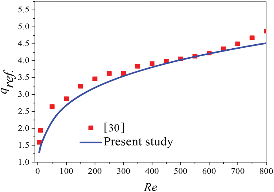
Figure 2: Comparison of the reference heat flux [30]
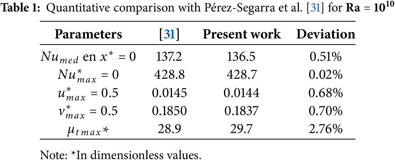
The results were solved and compared with those presented in Pérez-Segarra et al. to verify the code for turbulent flow in a closed cavity [31]. Table 1 compares the Nusselt number (Nu) values for their mean and maximum values. The maximum components of horizontal and vertical velocity were also compared. Lastly, the maximum turbulent viscosity was analyzed. The highest percentage difference was observed in the maximum turbulent viscosity, with a value of 2.76%. The other values compared exhibited a percentage difference of less than 1%, indicating a good approximation between results.
7 Calculation of Characteristic Parameters
The Nusselt number was calculated as Oosthuizen and Naylor [32],
And
The Sherwood number is defined as
Thermophysical Properties of the Mixture
The thermophysical properties of the mixture were not initially defined, necessitating their determination through a specific methodology. This methodology was extracted from sources [33–35]. First, the property of each element of the chemical compound was identified, and then the thermophysical properties were calculated for the new binary mixture.
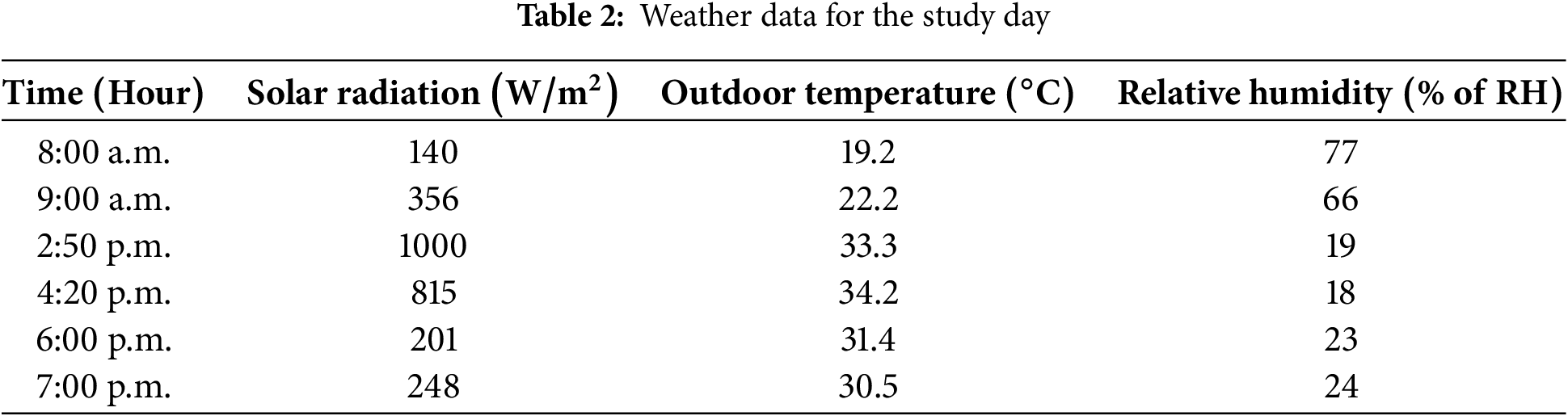
Below are the results of the numerical study of the thermal environment inside a greenhouse with different percentages of humidity concentration. Different Ra numbers were considered to vary the length dimensions of the greenhouse. The external weather conditions in the Amazcala area of Querétaro state were taken into account for a particular day: 24 June 2024. The National Meteorological Service (SMN) provided the weather data, which is an agency dependent on CONAGUA [36]. The weather data was considered for six different hours: 08:00 a.m., 09:00 a.m., 2:50 p.m., 4:20 p.m., 6:00 p.m. and 7:00 p.m. The study interval covered different climatic conditions throughout the day. For example, the minimum solar radiation was 140 w/m2, the maximum was 1000 w/m2, the minimum temperature recorded was 19.2°C, and the maximum temperature was 34.2°C. Regarding the relative humidity levels, the minimum value was 19% at 2:50 p.m., and the maximum was 77% at 08:00 a.m. The values of the external climate variables for the different hours are presented in Table 2.
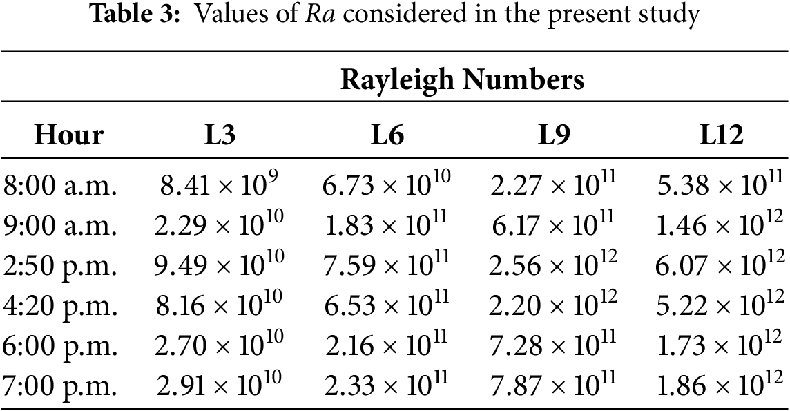
In Table 3, the Rayleigh number values corresponding to the different lengths of the greenhouse and the hours of the study day are represented. The greenhouse lengths were 3, 6, 9, and 12 m for a Rayleigh number range of 109 to 1012.
Two scenarios were presented for the hygrothermal study of the greenhouse. In the first case, the greenhouse was considered a closed cavity exposed to external weather conditions. As external weather conditions changed throughout the day, variations in solar radiation, external temperature, and relative humidity were considered. The internal temperature and relative humidity values were determined, considering the differentially heated cavity with a humidity concentration difference on the vertical walls. The results were presented steadily, showing the local and average temperature and relative humidity values.
A second scenario analyzed involved the same conditions as scenario one, with the addition of internal sources of humidity concentration placed equidistantly near the lower wall. Additionally, the number of humidity concentration sources increased with the greenhouse length.
8.1 Flow Patterns inside the 3 m Length Greenhouse
In Fig. 3, the flow patterns inside the greenhouse are shown for a Rayleigh number range of
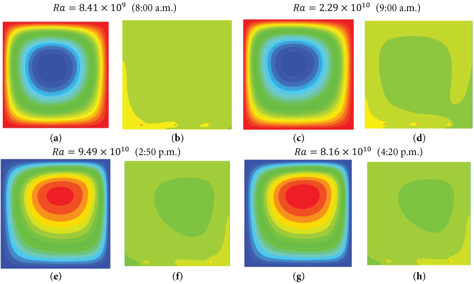
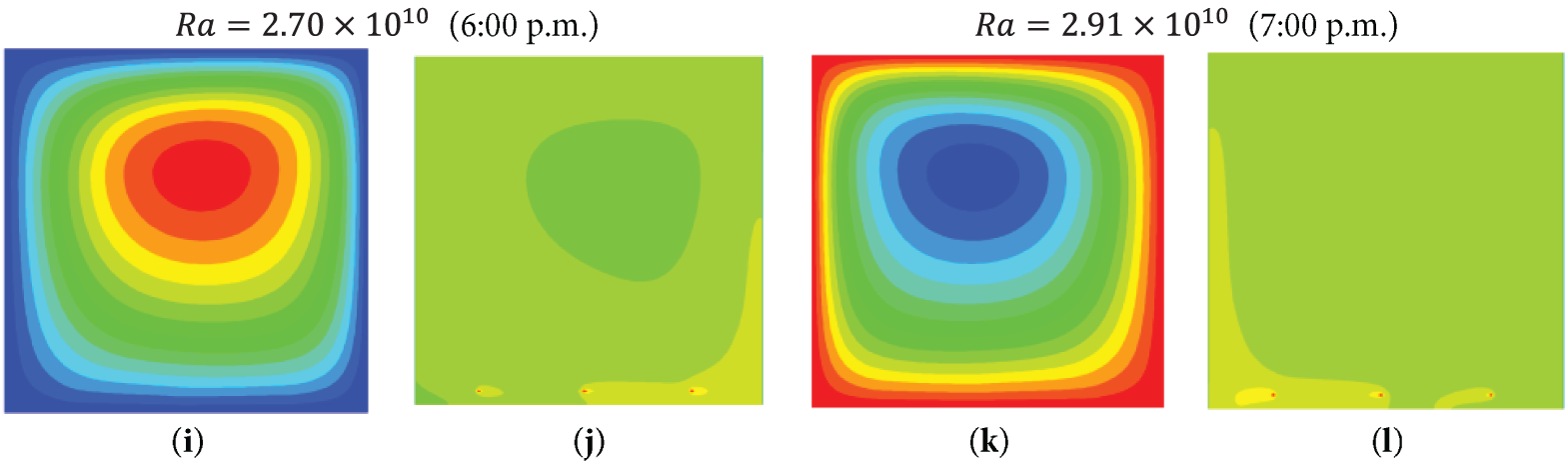
Figure 3: Flow patterns and contaminant concentration for different hours of the day with variation of the Rayleigh number, case L3. (a, c, e, g, i, k) heat transfer; (b, d, f, h, j, l) mass transfer
8.2 Velocity Components with and without Humidity Concentration Sources
In this section, an analysis of the flow pattern behavior through the velocity components is conducted. These velocity components were plotted along the central horizontal and vertical lines of the greenhouse. The velocity components were shown for the two scenarios of the case study: one, the greenhouse without internal humidity concentration sources, and two, the greenhouse with internal humidity concentration sources.
In Fig. 4, the velocity components at the center of the greenhouse are first shown. Fig. 4a,b presents the velocity components for the first case study. The velocity components showed eight values representing the six study hours throughout the day. The day hours ranged from 08:00 to 19:00. Fig. 4c,d represents the velocity components for the second case study. The greenhouse has three humidity concentration sources placed equidistantly from the vertical walls and at one-twelfth of the height. The vertical components shown in Fig. 4a exhibit recirculation behavior near the left vertical wall and the center of the greenhouse.
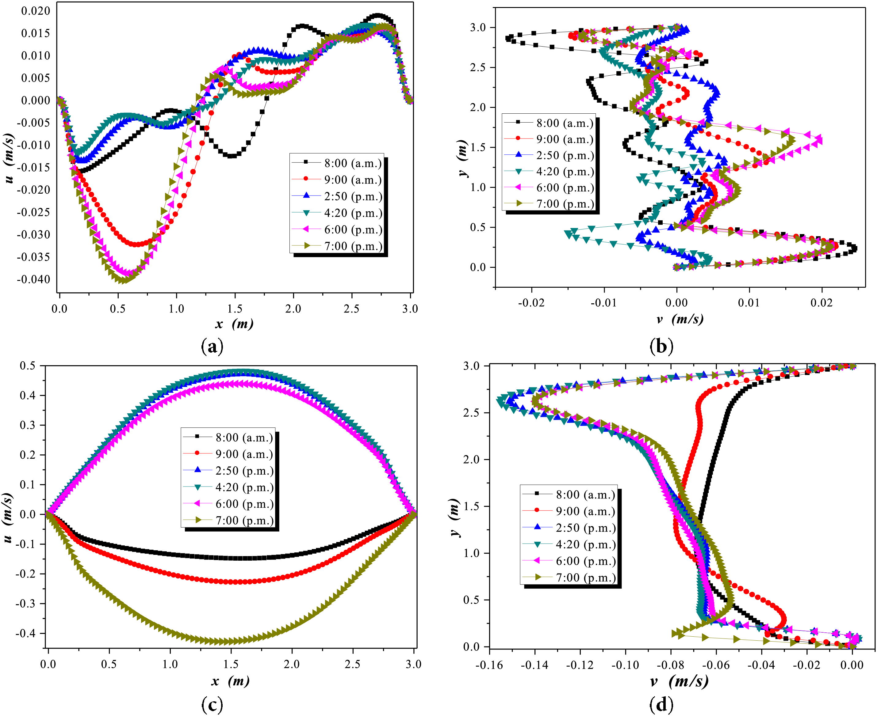
Figure 4: Velocity components during winter at 3 m: (a)
In contrast, the behavior shown in Fig. 4c differs significantly from that shown in Fig. 4a. In Fig. 4c, two groups in the velocity components are observed. The upper group appeared at 2:50, 4:20, and 6:00 p.m. The lower group appeared at 08:00 a.m., 09:00 a.m., and 7:00 p.m. The behavior exhibited by the velocity components was due to buoyancy forces generated by the humidity concentration sources placed inside the greenhouse. These humidity concentration sources inside the greenhouse caused changes in the flow recirculation. The flow pattern shown through the vertical velocity component in Fig. 4d was affected by an increase in intensity near the upper wall. Fig. 4 shows the two different behaviors of the two case studies, with the maximum velocity components appearing near the interior wall and the left wall when no diffusing sources are present inside.
In Fig. 5, the horizontal (a) and (c) and vertical (b) and (d) velocity components are shown for the two case studies: one without internal humidity concentration sources and one with internal humidity concentration sources, for a greenhouse length of 6 m. The behavior of the components in Fig. 5a,b without internal humidity concentration sources was due to small recirculation that formed in the central zone of the greenhouse interior. The second case with internal humidity concentration sources, shown in Fig. 5c,d, formed two recirculations inside the greenhouse at all study hours, except for 7:00 p.m., representing an elongated recirculation inside the cavity. It can be observed in the figures that the flow pattern changes as the length of the greenhouse increases. These results help determine the best conditions for operating the greenhouse, as each considered parameter affects the diffusion of heat or mass.
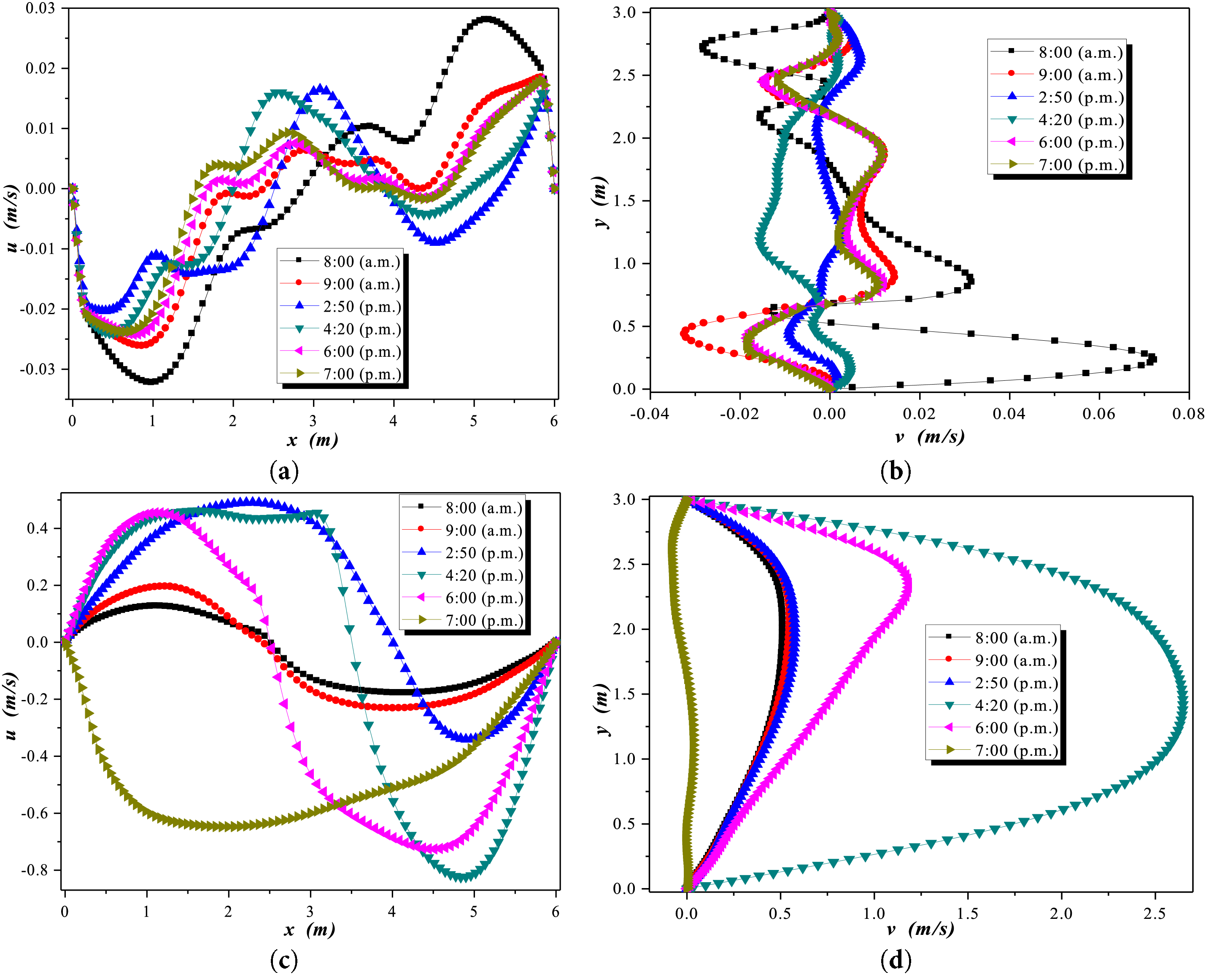
Figure 5: Velocity components during winter at 6 m: (a)
In Fig. 6, the velocity components at the center of the greenhouse with a length of 9 m are shown. Fig. 6a,b for the first case study demonstrated that at 2:50 p.m., there was a variation in flow intensity due to the maximum received radiation. At 08:00 a.m., small recirculations formed in the center of the greenhouse. At 09:00 a.m., two small recirculations merged in the center of the greenhouse. At 2:50 p.m., an elongated recirculation formed in the center of the greenhouse. At 4:20 p.m., two small recirculations in the center of the greenhouse changed their circulation direction. At 6:00 and 7:00 p.m., a recirculation similar to that observed at 09:00 reappeared. The described behavior was due to changes in solar radiation and external temperature conditions.
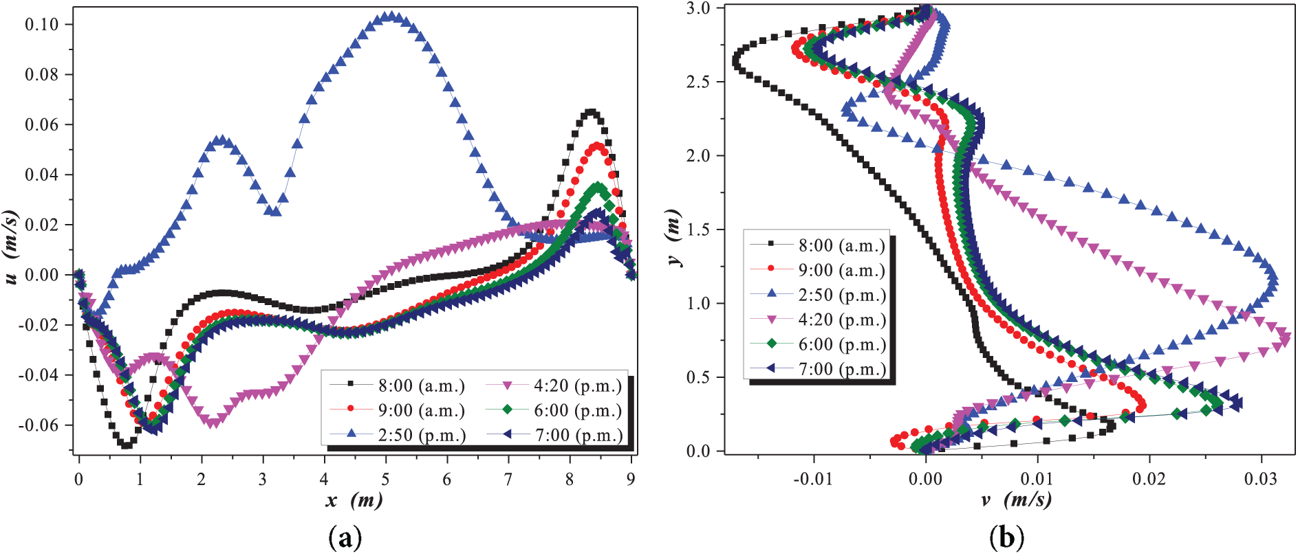
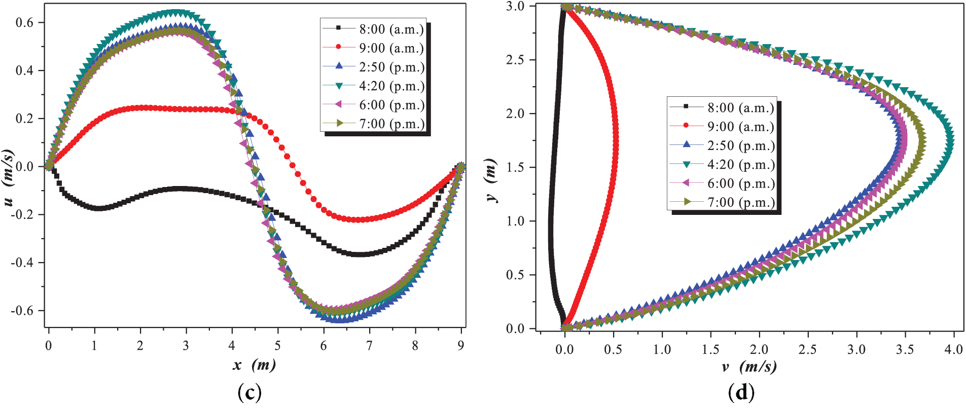
Figure 6: Velocity components during winter at 9 m: (a)
In Fig. 6c,d, a symmetrical behavior in the recirculations after 2:50 p.m. can be observed, with lower velocities in the morning hours due to lower radiation. It is notable that in Fig. 6d, the velocity behavior is parabolic after 2:50 p.m., indicating that velocities reach a maximum at the greenhouse’s mid-height. At 8:00 a.m. and 9:00 a.m., the velocities are low, suggesting few recirculations. Additionally, in Fig. 6a,b, dispersed flow patterns with prominent velocity components at 2:50 p.m. were observed. Conversely, in Fig. 6c,d, the velocity components follow a uniform pattern due to the predominant convective intensity exerted by the humidity sources.
Finally, in Fig. 7a,b, it was observed that the velocity components tend to have extreme values. This change was due to the increase in the greenhouse length, which was considered to be 12 m. Consequently, the flow recirculations have also increased. In Fig. 7c,d, the flow pattern is divided into two groups: the predominant group on the left side and the one on the right side. It can be observed that the vertical velocity component values reach their maximum at the mid-height of the cavity at 2:50 p.m. The horizontal component behavior took on a parabolic shape, indicating that the highest velocity values at all study hours were at the mid-height of the greenhouse.
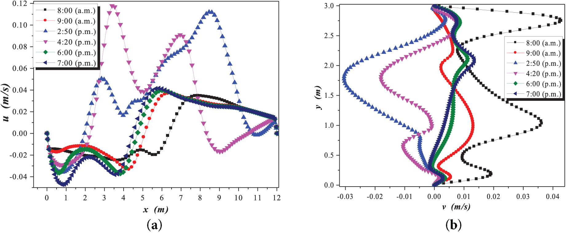
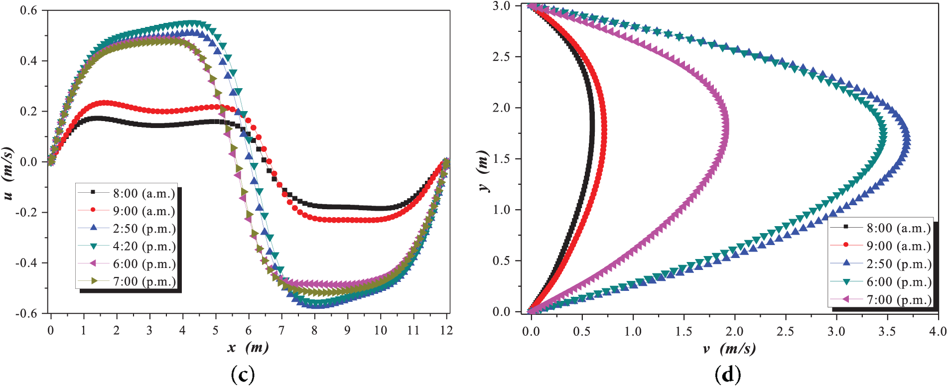
Figure 7: Velocity components during winter at 12 m: (a)
8.3 Flow Patterns inside a 9 m Length Greenhouse
The flow patterns shown in Fig. 8 illustrate the behavior of heat flow at different hours of the day. First, the flow pattern is shown, and below it, the behavior of humidity concentration is displayed. It can be observed that in all cases, a mushroom-shaped dispersion formed at different hours of the day. However, the flow pattern remained similar, indicating that the flow recirculation remained in two groups, one on each side of the greenhouse.

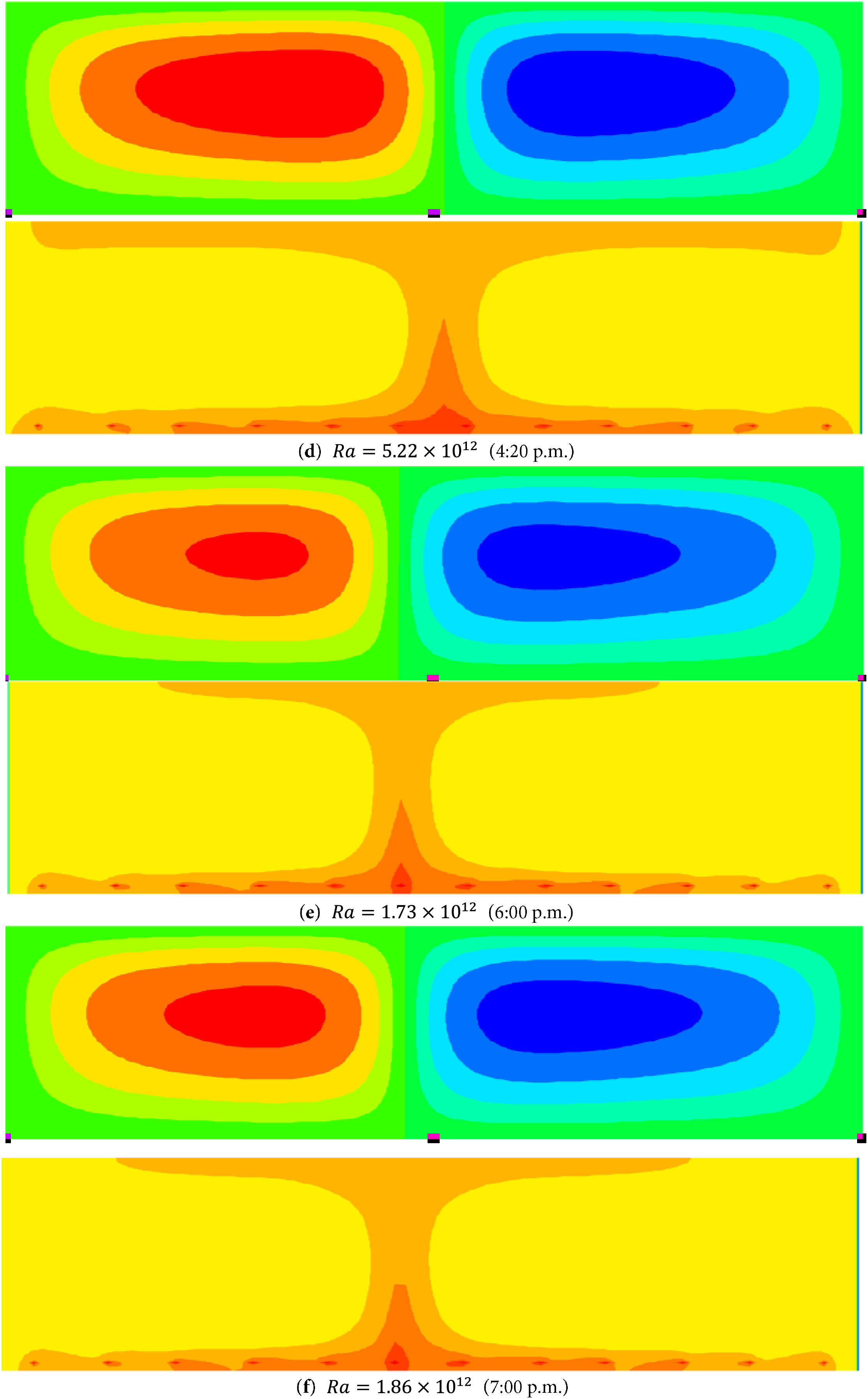
Figure 8: Flow patterns of heat and mass transfer throughout the day for different Rayleigh numbers, Case 12. (a–f) heat transfer (above) and mass transfer (below)
The behavior of temperatures and humidity concentration inside the greenhouse for the two case studies, with and without internal humidity sources, is shown below. In Fig. 9a,b, the temperature values are displayed, and a significant difference can be observed when internal humidity sources are not considered. The lowest temperature value shown in Fig. 9a was at 8:00 a.m., with a value of 20.5°C. A group of temperature values is observed in the range of 21.5°C to 32°C. The last group of temperature values is between 44.5°C and 50.5°C. These values were recorded as the length of the greenhouse increased.
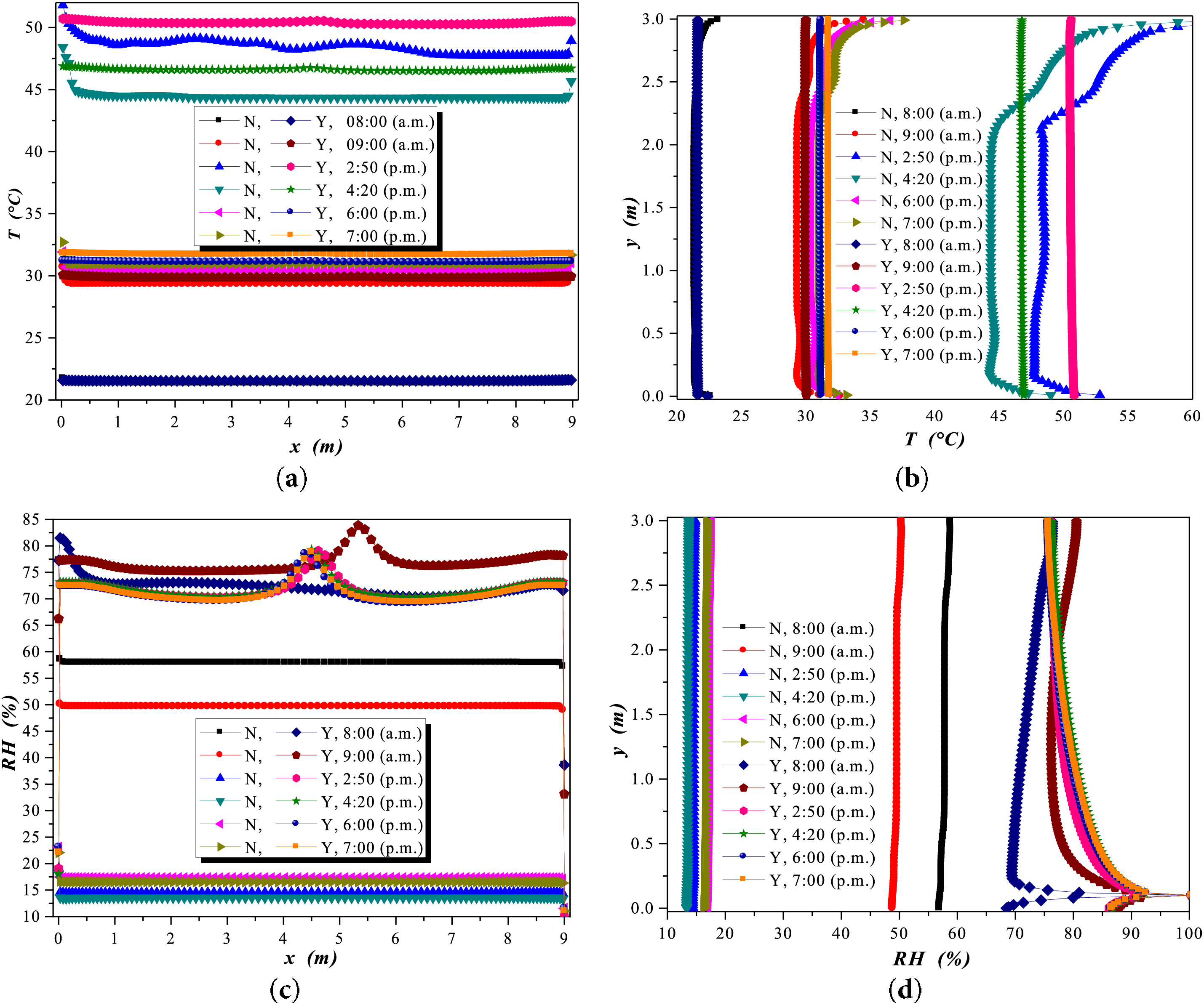
Figure 9: Central variations inside the greenhouse along length and height considering “Y” (with) and “N” (without) humidity sources: (a, b) temperatures, (c, d) RH percentages
Regarding temperature variation with height inside the greenhouse, as shown in Fig. 9b, the lowest temperatures were recorded at 8:00 a.m. A group of temperatures with a difference of less than 3°C is observed for all hours of the day, i.e., from 8:00 a.m. to 7:00 p.m., but with internal humidity sources inside the greenhouse. These values are in the range of 29.3°C to 31.8°C. For temperature values without internal humidity sources inside the greenhouse, variations between 44.3°C and 50.5°C were recorded at 2:50 and 4:20 p.m. At the same time, there were temperature variations with and without internal humidity sources.
The relative humidity values are shown in Fig. 9c,d. In this case, all values are below 58% RH when no humidity sources are considered from 8:00 a.m. to 7:00 p.m. The other group with humidity sources is between 72% RH and 85% RH, with the highest values near the right wall of the greenhouse. In locations near the floor (10 cm height) where humidity sources are located, values above 90% RH were found.
Table 4 presents the average temperature values inside the greenhouse at different hours of the day for the most extensive geometry case study. The lowest recorded temperature was 21.52°C at 8:00 a.m., and the highest was 50.15°C at 2:50 p.m.
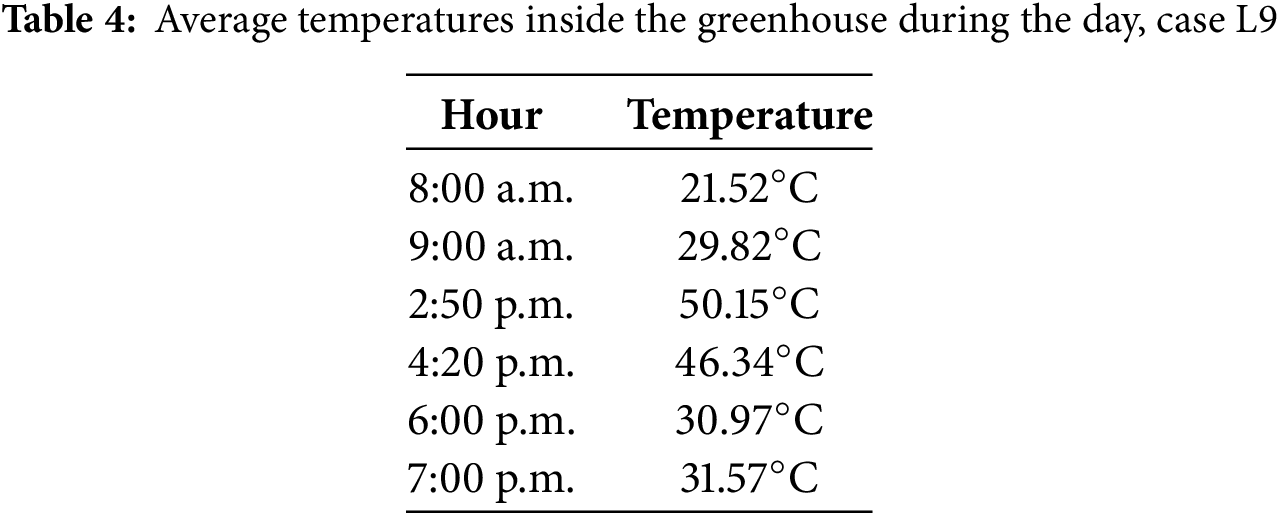
Table 5 shows the results of the relative humidity concentrations inside the greenhouse for the last case study with the L9 geometry. The RH values for all study hours are displayed, and it can be observed that when ten humidity sources are placed, the humidity percentages are insignificant compared to the case without RH sources. These values show a difference of less than 0.5%. As the number of RH sources increases, the humidity becomes more homogenized, reaching the highest values when considering 100 RH sources. The RH values range from 83.26% to 86.62%, with the highest value reached at 8:00 a.m.
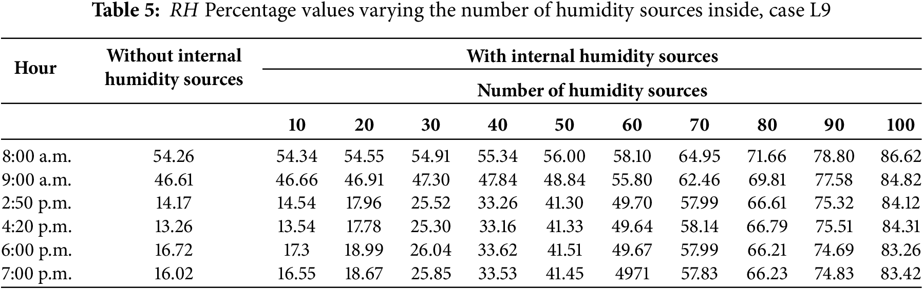
Fig. 10 presents the values of the convective and radiative Nusselt numbers to understand the behavior of convective heat transfer inside the greenhouse. The values for the two vertical walls, the left and right, are shown. It can be observed that when considering the radiative effect (radiative Nusselt), it is 70% higher compared to the highest value of the convective Nusselt. Notably, the highest value of the convective Nusselt was recorded at 8:00 a.m., while the highest value of the radiative Nusselt was recorded at 2:50 p.m. This makes sense as it corresponds to the time of the highest radiation.
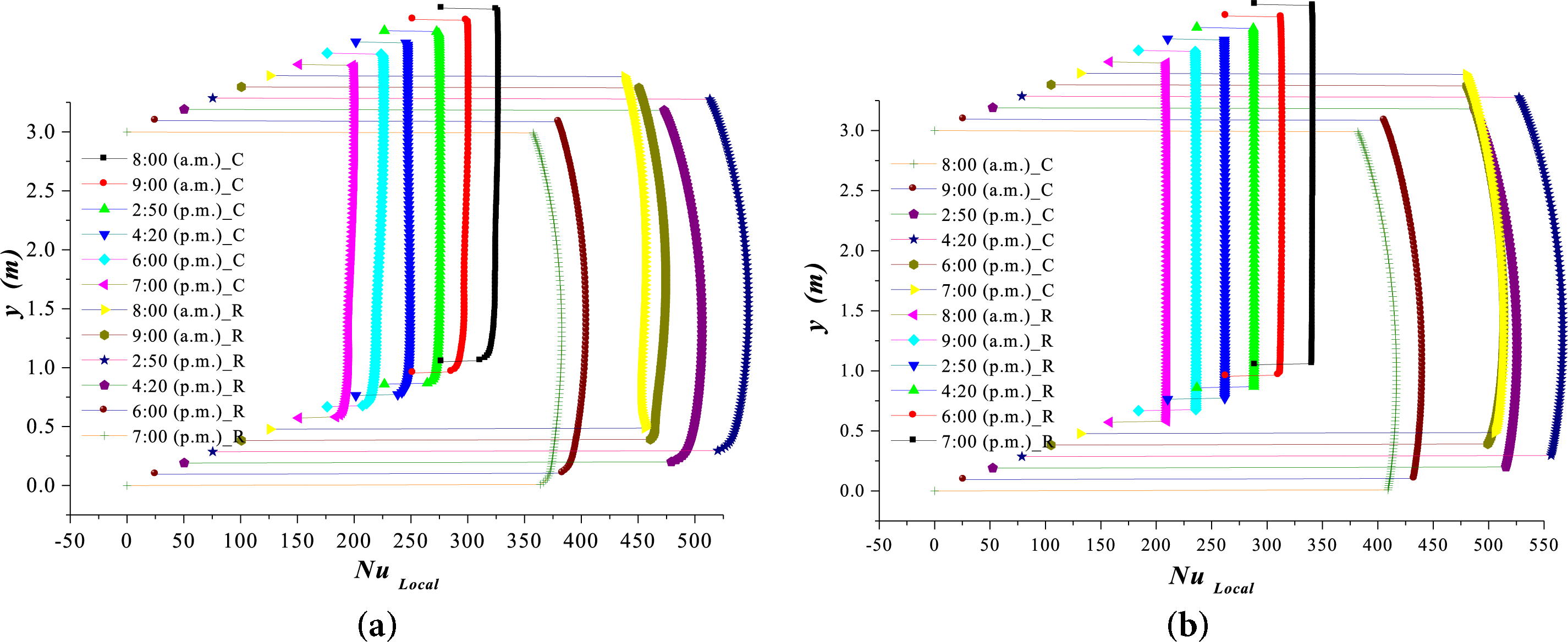
Figure 10: Values of convective Nusselt number “C” and Radiative Nusselt number “R”, (a) left wall and (b) right wall
8.4 Convective and Radiative Nusselt with and without Humidity Sources
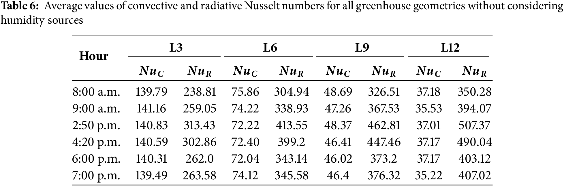
To better understand the authors’ discussion on the behavior of convective and radiative heat transfer inside the greenhouse, Table 6 presents the values of the convective and radiative Nusselt numbers for the case without internal humidity sources across the four different geometries considered in this research. In each case, it can be observed that the radiative Nusselt number is always higher, with the highest recorded value of 507.37 at 2:50 p.m., in L12. The contrast arises because the lowest convective Nusselt values are presented in this L12 case. The highest convective Nusselt values occur in L3, indicating that convective heat transfer decreases with increased greenhouse dimensions.
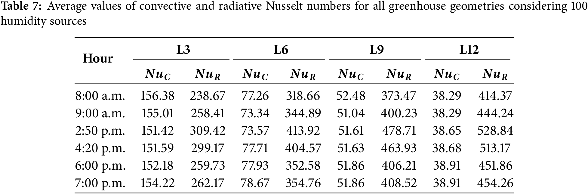
On the other hand, comparing the convective and radiative Nusselt values considering humidity sources inside for the different study cases from L3 to L12, as shown in Table 7, the increase in the maximum radiative Nusselt value of 528.84 is insignificant compared to the case without humidity sources, with an increase of less than 0.05%. Notably, convective heat transfer increases when RH sources are inside the greenhouse. However, the highest values occur at different hours of the day. This is not the case for the highest radiative Nusselt values, which occur at 2:50 p.m.
For the mass transfer analysis, Fig. 11 presents the cases for different humidity concentrations inside the greenhouse. The mass transfer is analyzed by varying the number of humidity sources inside the greenhouse, starting with ten humidity sources and increasing by increments of 10 up to 100 humidity sources. The analysis showed that when there are only ten humidity sources at any hour of the study day, the convective mass transfer remains constant after a height of 0.25 m inside the greenhouse.
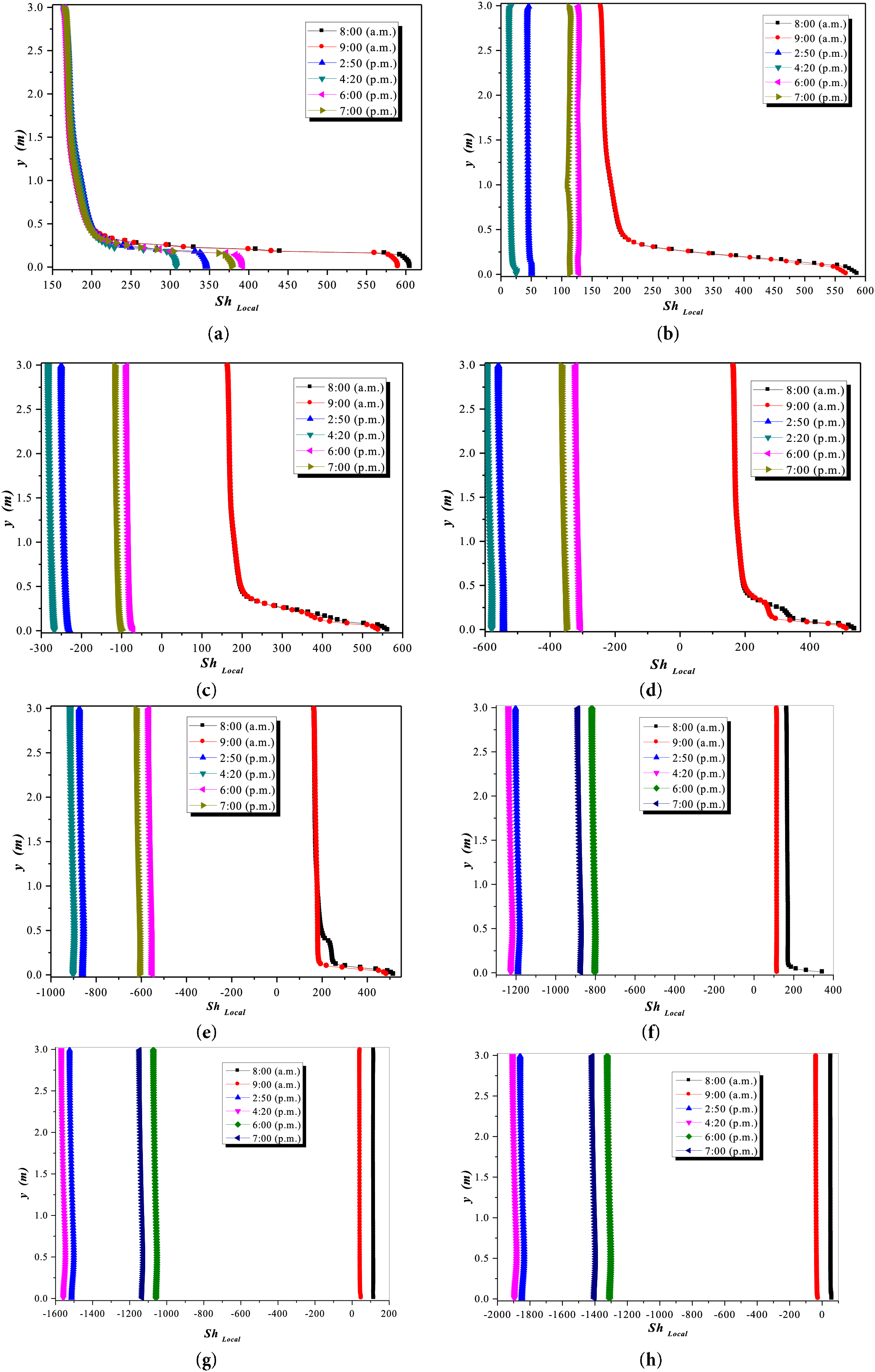
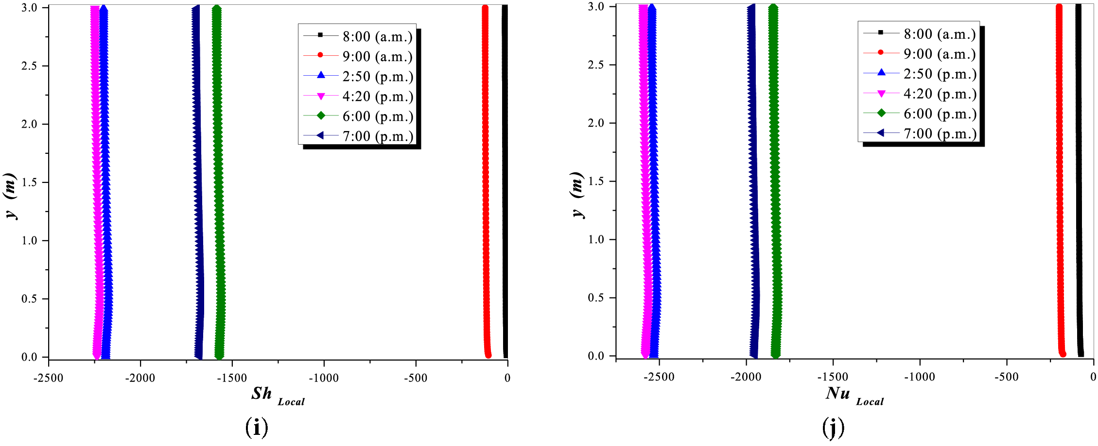
Figure 11: Values of convective Nusselt number considering different humidity concentrations inside the greenhouse, (a) 10 humidity sources, (b) 20 humidity sources, (c) 30 humidity sources, (d) 40 humidity sources, (e) 50 humidity sources, (f) 60 humidity sources, (g) 70 humidity sources, (h) 80 humidity sources, (i) 90 humidity sources, and (j) 100 humidity sources
In contrast, in other cases, for example, Fig. 11b shows that the convective effect has increased, being maximal at 8:00 and 9:00 a.m. This behavior remains similar for 30, 40, and 50 humidity sources. However, in case (f), the convective effect decreases, and a difference is noticeable between 8:00 and 9:00 h. In all cases, it can be observed that after 20 humidity sources inside, the maximum convective effect occurs at 2:50 and 4:20 p.m. Notably, as the number of humidity sources increases, the convective impact also increases. However, the direction of the convective movement is also reversed.
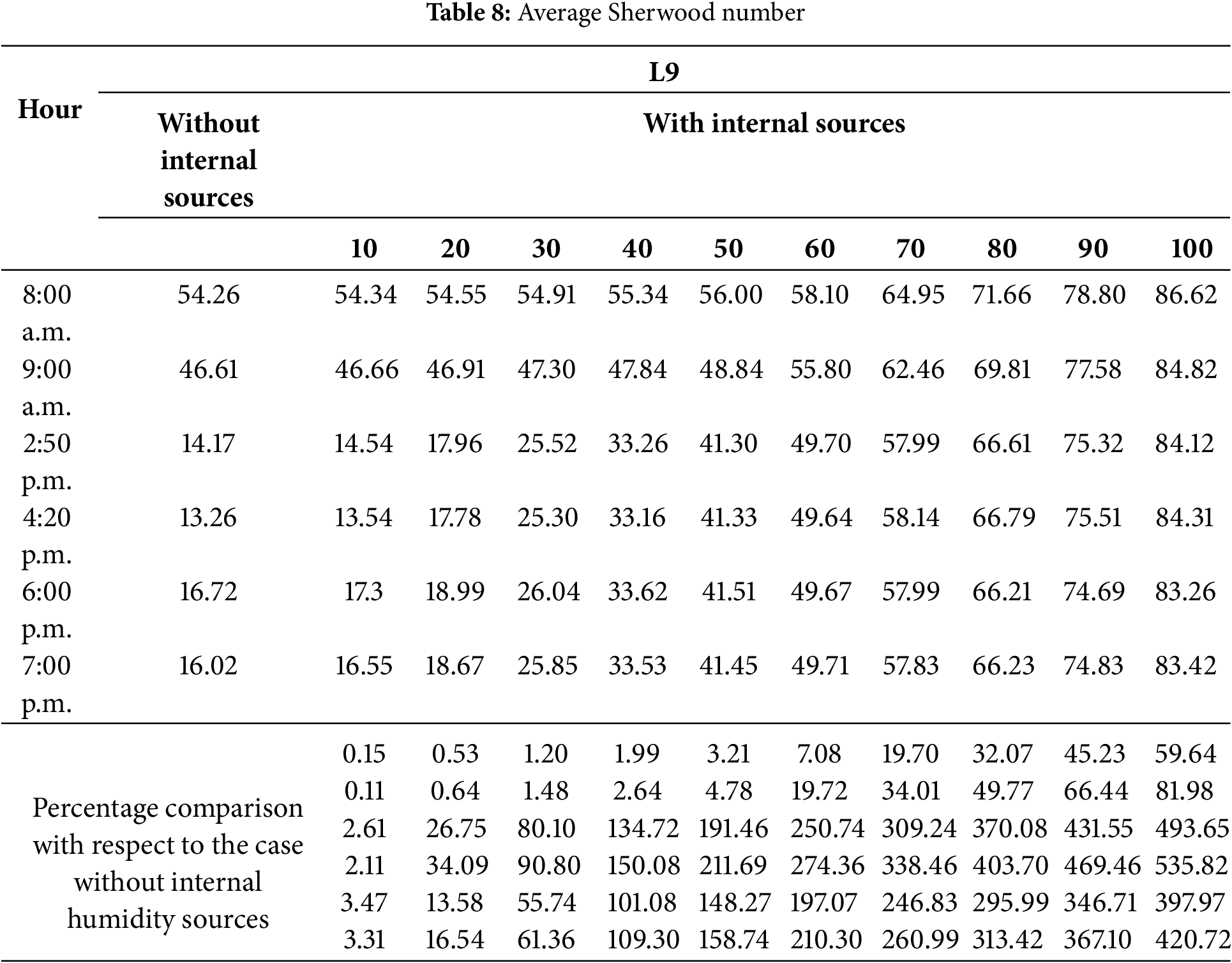
Table 8 presents the average values of the Sherwood number (Sh). It is observed that without humidity sources, the highest values start at 8:00 a.m. and decrease in the afternoon to 7:00 p.m. with a value of 16.02. As the number of humidity sources increases, the convective mass effect increases until a practically constant impact is achieved with a large number of humidity sources. In Table 8, the percentage difference can also be observed when humidity sources are placed, and their number is incremented. The percentage is sensitive to the increase of two parameters: one, the number of humidity sources, and two, the time of day.
A numerical study was conducted covering many parameters that define the hygrothermal conditions inside the greenhouse. This study provides valuable information for understanding the behavior of complex phenomena such as heat and mass transfer. The parameters analyzed included greenhouse dimensions related to changes in the Rayleigh number. Two cases were considered: one without internal humidity sources and the second with internal humidity sources. In the second case, the number of internal humidity sources inside the greenhouse was varied to observe the convective mass effect. Different solar radiation intensities were also considered to understand their daily effect. The results were intriguing, and the analysis yielded several conclusions. Here are the most relevant ones.
• In each hour of the study, four geometries were analyzed. With the smallest geometry of 3 m in length, a change in direction in the flow was observed over the day, showing in the first two hours and the last hour, according to Fig. 3, the heat is concentrated around the envelopes. This process indicates that the radiation directly affects the surrounding surfaces, and subsequently, the heat is transported to the center of the cavity. The effect of moisture transport is similar, but to a lesser extent. The goal was to combine both effects to provide the necessary heat and humidity inside the greenhouse.
• The behavior of the flow pattern can be deduced from the analysis of the velocity components because they show how recirculations are formed and in which directions the velocities intensify at different times of the day. For the 3 m geometry, the flow distribution without internal sources shows that the velocity components intensify at 0.5 m from the hot wall. When there are internal sources, recirculations are created, which are dominated by the radiation intensity.
• By increasing the greenhouse length to 6 m, fluid movement without internal sources intensifies at a height of 0.5 m, creating a homogeneous distribution. The fluid movement rises to a maximum value at 4:20 p.m. by placing the internal sources.
• By increasing the length to 9 m, the flow pattern achieves recirculation when there are internal sources. The y-velocity components increase from 2:50 p.m. onwards.
• Finally, at a length of 12 m, the movement of the fluid has the lowest speed of 0.4 m/s. This benefits the greenhouse’s interior by achieving a homogeneous distribution; however, by placing the interior sources of humidity, the speeds increase, and recirculations are formed. The highest speeds are reached in the center of the greenhouse at a height of 1.5 m. When the greenhouse length is increased, two recirculations are formed that are intensified by the radiation that is incident on the wall surfaces. These two recirculations are in opposite directions, one with a higher temperature than the other.
In analyzing temperatures and concentrations along the length and height of the greenhouse in its central coordinate, temperatures increase considerably when moisture sources inside are not considered, reaching the maximum temperature of 50.15°C by 2:50 p.m. The lowest temperature was 21.52°C at 8:00 a.m.
• By increasing the number of moisture sources, the humidity in the air is saturated in such a way that when there are 100 humidity sources, it becomes homogeneous, on average 85% in all the study hours. This analysis provides insight into determining the desired humidity percentages for the number of moisture sources.
• The heat transfer analyzed through the Nusselt number shows an increase from 16.02°C at 7:00 p.m. to the highest value of 54.26°C at 8:00 p.m. It is observed that in the case of humidity sources inside, the Nusselt number tends to be homogeneous at any time, as the number of humidity sources increases.
• The convective and radiative Nusselt numbers show that the convective contribution decreases with increasing greenhouse length, and the opposite happens for the radiative contribution. This demonstrates the importance of these studies because, generally, only the convective effect is considered in other studies. Here, the maximum radiative Nusselt was 507.37 at 2:50 p.m., and the highest average was 528.84 for the cavity length of 12 m.
• The Sherwood number was found to change according to the time of day, presenting the smallest value of 13.26 at 4:20 p.m., when sources of humidity are not considered. When humidity sources are considered, the highest values occur in the morning, obtaining the most significant value of 86.62 at 8:00 a.m.
This study explores heat and mass transfer in greenhouses, highlighting the importance of integrating convective and radiative effects in environmental control. By analyzing different geometries, internal moisture sources, and solar radiation intensities, practical strategies for achieving optimal hygrothermal conditions are presented. The findings show how greenhouse length, humidity sources, and flow patterns influence temperature distribution, humidity, and air circulation distribution.
Greenhouse geometry is critical in shaping flows and recirculations, especially with internal moisture sources. Larger greenhouses favor uniform conditions, although radiative recirculations generate variability. In addition, the relevance of the radiative Nusselt number, often ignored in previous studies, is highlighted as a critical factor in heat transfer. These results establish a basis for designing more efficient and productive greenhouses. Future studies could explore the interaction of these parameters in different climates to generalize the findings and optimize design strategies.
In future work, it is considered to place the measuring devices in the study prototype to perform the measurements and to be able to compare the experimental and numerical results.
Acknowledgement: We would like to extend our special thanks to SECIHTI (Secretariat of Science, Humanities, Technology, and Innovation) for awarding M. I. Hernández-López a grant to develop the research project related to this study. We would also like to thank TecNM-Campus Pachuca for its support in financing the publication costs.
Funding Statement: The authors received no specific funding for this study.
Author Contributions: The authors confirm contribution to the paper as follows: study conception and design: J. Serrano-Arellano, K. M. Aguilar-Castro; data collection: M. I. Hernández-López, E. V. Macias-Melo, J. L. Chávez-Servín; analysis and interpretation of results: J. Serrano-Arellano, E. V. Macias-Melo, M. I. Hernández-López; draft manuscript preparation: K. M. Aguilar-Castro, J. Serrano-Arellano, J. L. Chávez-Servín. All authors reviewed the results and approved the final version of the manuscript.
Availability of Data and Materials: The data that support the findings of this study are available from the corresponding author, K. M. Aguilar-Castro, upon reasonable request.
Ethics Approval: Not applicable.
Conflicts of Interest: The authors declare no conflicts of interest to report regarding the present study.
References
1. Paing ST, Anderson TN. Characterising the effects of geometry on the natural convection heat transfer in closed even-span gable-roof greenhouses. Therm Sci Eng Prog. 2024;48:102408. doi:10.1016/j.tsep.2024.102408. [Google Scholar] [CrossRef]
2. Yanru L, Yubin J, Si W, Xin L, Wenxin L, Müslüm A, et al. Spatial temperature distribution and ground thermal storage in the plastic greenhouse: an experimental and modeling study. J Energy Storage. 2024;77:109938. doi:10.1016/j.est.2023.109938. [Google Scholar] [CrossRef]
3. Çam NY, Ezan MA, Biçer Y. Transient thermal modelling of a Mediterranean greenhouse for sustainable agriculture: comparison of desert and dry-summer subtropical climates. Sol Energy. 2024;268:112280. doi:10.1016/j.solener.2023.112280. [Google Scholar] [CrossRef]
4. Mao C, Su Y. CFD based heat transfer parameter identification of greenhouse and greenhouse climate prediction method. Therm Sci Eng Prog. 2024;49:102462. doi:10.1016/j.tsep.2024.102462. [Google Scholar] [CrossRef]
5. Almashharawi A, Bamasag A, Abulkhair H, Lefers R. Pilot study on liquid desiccant systems in greenhouse for water saving and climate control. Case Stud Therm Eng. 2024;61:105165. doi:10.1016/j.csite.2024.105165. [Google Scholar] [CrossRef]
6. Mao Q, Li H. Simulation of ambient temperature and humidity distribution in eight-span greenhouse under different wind conditions and corn height. Case Stud Therm Eng. 2024;61:105099. doi:10.1016/j.csite.2024.105099. [Google Scholar] [CrossRef]
7. Mardomakdeh SM, Poshtiri AH, Farahani M. A numerical study of cucurbit cultivation in a greenhouse under direct solar radiation and equipped with a direct evaporative cooler in summer season. Energy. 2024;292:130476. doi:10.1016/j.energy.2024.130476. [Google Scholar] [CrossRef]
8. Guo J, Liu Y, Lü E. Numerical simulation of temperature decrease in greenhouses with summer water-sprinkling roof. Energies. 2019;12(12):2435. doi:10.3390/en12122435. [Google Scholar] [CrossRef]
9. An C-H, Ri H-J, Han T-U, Kim S-I, Ju U-S. Feasibility of winter cultivation of fruit vegetables in a solar greenhouse in temperate zone; experimental and numerical study. Sol Energy. 2022;233(4):18–30. doi:10.1016/j.solener.2022.01.024. [Google Scholar] [CrossRef]
10. Zhang G, Shi Y, Liu H, Fei Z, Liu X, Wei M, et al. Heat transfer performance of an assembled multilayer wall in a Chinese solar greenhouse considering humidity. J Energy Storage. 2021;33(1):102046. doi:10.1016/j.est.2020.102046. [Google Scholar] [CrossRef]
11. Kavga A, Thomopoulos V, Pischinas E, Tsipianitis D, Nikolakopoulos P. Design and simulation of a greenhouse in a computational environment (ANSYS/FLUENT) and an automatic control system in a LABVIEW environment. Simul Model Pract Theory. 2023;129:102837. doi:10.1016/j.simpat.2023.102837. [Google Scholar] [CrossRef]
12. Saberian A, Sajadiye SM. The effect of dynamic solar heat load on the greenhouse microclimate using CFD simulation. Renew Energy. 2019;138(9):722–37. doi:10.1016/j.renene.2019.01.108. [Google Scholar] [CrossRef]
13. Carlini M, Castellucci S, Mennuni A, Morelli S. Numerical modeling and simulation of pitched and curved-roof solar greenhouses provided with internal heating systems for different ambient conditions. Energy Rep. 2020;6(1):146–54. doi:10.1016/j.egyr.2019.10.033. [Google Scholar] [CrossRef]
14. Han F, Chen C, Hu Q, He Y, Wei S, Li C. Modeling method of an active–passive ventilation wall with latent heat storage for evaluating its thermal properties in the solar greenhouse. Energy Build. 2021;238(6):110840. doi:10.1016/j.enbuild.2021.110840. [Google Scholar] [CrossRef]
15. Wang J, Lee WF, Ling PP. Estimation of thermal diffusivity for greenhouse soil temperature simulation. Appl Sci. 2020;10(2):653. doi:10.3390/app10020653. [Google Scholar] [CrossRef]
16. Ghani S, El-Bialy EMAA, Bakochristou F, Rashwan MM, Abdelhalim AM, Ismail SM. Pratheesh Ben, Experimental and numerical investigation of the thermal performance of evaporative cooled greenhouses in hot and arid climates. Sci Technol Built Environ. 2019;0(2):1–20. doi:10.1080/23744731.2019.1634421. [Google Scholar] [CrossRef]
17. Taki M, Ajabshirchi Y, Ranjbar SF, Rohani A, Matloobi M. Modeling and experimental validation of heat transfer and energy consumption in an innovative greenhouse structure. Inf Process Agric. 2016;3(3):157–74. doi:10.1016/j.inpa.2016.06.002. [Google Scholar] [CrossRef]
18. Tong G, Christopher DM, Li B. Numerical modelling of temperature variations in a Chinese solar greenhouse. Comput Electron Agric. 2009;68:129–39. doi:10.1016/j.compag.2009.05.004. [Google Scholar] [CrossRef]
19. Yu G, Zhang S, Li S, Zhang M, Benli H, Wang Y. Numerical investigation for effects of natural light and ventilation on 3D tomato body heat distribution in a Venlo greenhouse. Inf Process Agric. 2023;10(4):535–46. doi:10.1016/j.inpa.2022.05.006. [Google Scholar] [CrossRef]
20. Abid H, Ketata A, Lajnef M, Chiboub H, Driss Z. Numerical investigation of greenhouse climate considering external environmental factors and crop position in Sfax central region of Tunisia. Sol Energy. 2023;264(12):112032. doi:10.1016/j.solener.2023.112032. [Google Scholar] [CrossRef]
21. Xiao J, Wang Q, Wang X, Hu Y, Cao Y, Li J. An earth-air heat exchanger integrated with a greenhouse in cold-winter and hot-summer regions of northern China: modeling and experimental analysis. Appl Therm Eng. 2023;232:120939. doi:10.1016/j.applthermaleng.2023.120939. [Google Scholar] [CrossRef]
22. Jehhef KA, Sattar Khdair MA, Jabbar Thajeel K. Numerical modeling of thermal radiation heat transfers in agricultural greenhouse. Mater Sci Eng. 2020;745(1):012072. doi:10.1088/1757-899x/745/1/012072. [Google Scholar] [CrossRef]
23. Gomez-Zavaglia A, Mejuto JC, Simal-Gandara J. Mitigation of emerging implications of climate change on food production systems. Food Res Intern. 2020;134(7):109256. doi:10.1016/j.foodres.2020.109256. [Google Scholar] [PubMed] [CrossRef]
24. Zeroual S, Bougoul S, Benmoussa H. Effect of radiative heat transfer and boundary conditions on the airflow and temperature distribution inside a heated tunnel greenhouse. J Appl Mech Tech Phys. 2018;59(6):1008–14. doi:10.1134/s0021894418060068. [Google Scholar] [CrossRef]
25. Serrano-Arellano J, Xamán J, Álvarez G, Gijón-Rivera M. Heat and mass transfer by natural convection in a square cavity filled with a mixture of Air–CO2. Int J Heat Mass Transf. 2013;64(11):725–34. doi:10.1016/j.ijheatmasstransfer.2013.05.038. [Google Scholar] [CrossRef]
26. Serrano-Arellano J, Belman-Flores JM, Xamán J, Aguilar-Castro KM, Macías-Melo EV. Numerical study of the double diffusion natural convection inside a closed cavity with heat and pollutant sources placed near the bottom wall. Energies. 2020;13(12):3085. doi:10.3390/en13123085. [Google Scholar] [CrossRef]
27. Henkes RAWM, Van Der Vlugt FF, Hoogendoorn CJ. Natural-convection flow in a square cavity calculated with low-Reynolds-number turbulence models. Int J Heat Mass Transf. 1991;34(2):377–88. doi:10.1016/0017-9310(91)90258-g. [Google Scholar] [CrossRef]
28. Siegel R, Howell J. Thermal radiation heat transfer. New York, NY, USA: Taylor and Francis; 1981. doi:10.1201/9780429327308. [Google Scholar] [CrossRef]
29. Patankar SV. Numerical heat transfer and fluid flow. New York, NY, USA: McGraw-Hill, Hemisphere Publishing Co.; 1980. [Google Scholar]
30. Raji A, Hasnaoui M. Mixed convection heat transfer in a rectangular cavity ventilated and heated from the side. Numer Heat Transf. 1998;33:533–48. doi:10.1080/10407789808913953. [Google Scholar] [CrossRef]
31. Pérez-Segarra C, Oliva A, Costa M, Escanes F. Numerical experiments in turbulent natural and mixed convection in internal flows. Int J Num Meth Heat Fluid Flows. 1995;5(1):13–33. doi:10.1108/eum0000000004114. [Google Scholar] [CrossRef]
32. Oosthuizen P, Naylor D. Introduction to convective heat transfer analysis. New York, NY, USA: McGraw-Hill; 1999. [Google Scholar]
33. Reid RC, Prausnitz JM, Poling BE. The properties of gases and liquids. New York, NY, USA: McGraw-Hill; 1987. [Google Scholar]
34. Bird RB, Stewart WE, Lightfoot EN. Transport phenomena. 2nd ed. Hoboken, NJ, USA: John Wiley & Sons, Inc.; 2006. [Google Scholar]
35. Perry RH. Perry’s chemical engineers handbook. New York, NY, USA: McGraw-Hill; 1997. [Google Scholar]
36. Comisión Nacional del Agua (CONAGUAInformación estadística climatológica, Servicio Meteorológico Nacional, México. [cited 2024 Nov 21]. Available from: https://smn.conagua.gob.mx/es/climatologia/informacion-climatologica/informacion-estadistica-climatologica. [Google Scholar]
Cite This Article
 Copyright © 2025 The Author(s). Published by Tech Science Press.
This work is licensed under a Creative Commons Attribution 4.0 International License , which permits unrestricted use, distribution, and reproduction in any medium, provided the original work is properly cited.
 Downloads
 Citation Tools